the Creative Commons Attribution 4.0 License.
the Creative Commons Attribution 4.0 License.
 | 09 Nov 2022
Impulse-driven oscillations of the near-Earth's magnetosphere
Hiroatsu Sato
Jan Trulsen
Per Even Sandholt
Charles Farrugia
It is argued that a simple model based on magnetic image arguments suffices to give a convincing insight into both the basic static as well as some transient dynamic properties of the near-Earth's magnetosphere, particularly accounting for damped oscillations being excited in response to impulsive perturbations. The parameter variations of the frequency are given. Qualitative results can also be obtained for heating due to the compression of the radiation belts. The properties of this simple dynamic model for the solar wind–magnetosphere interaction are discussed and compared to observations. In spite of its simplicity, the model gives convincing results concerning the magnitudes of the near-Earth's magnetic and electric fields. The database contains ground-based results for magnetic field variation in response to shocks in the solar wind. Here, the observations also include data from the two Van Allen satellites.
- Article
(15427 KB) - Full-text XML
- BibTeX
- EndNote


Instrumented spacecraft in the near-Earth's magnetosphere detect significant dynamic variations in the magnetic fields and plasma properties in response to variations in the solar wind (Araki, 1994; Araki et al., 1997; Archer et al., 2013; Blum et al., 2021). The abrupt increase in pressure associated with interplanetary (IP) shocks that are driven, for instance, by interplanetary coronal mass ejections (ICMEs) will compress the low-latitude geomagnetic field through an intensification of the Chapman–Ferraro magnetopause current. This leads to a sudden impulse (SI) which can also be observed in low-latitude magnetometer records. It was demonstrated (Farrugia and Gratton, 2011) that such SI events are often followed by oscillations of ∼5 min periods. These can also be observed by satellites in the cold, dense magnetosheath and the hot and tenuous magnetospheric plasmas, also consistent with other related observations (Araki et al., 1997; Plaschke et al., 2009). The presence of magnetic pulsations with periods of 8-10 min measured by geosynchronous satellites are found to be well correlated with variations in the solar wind dynamic pressure (Kivelson et al., 1984; Sibeck et al., 1989; Korotova and Sibeck, 1995).
A simple dynamic model for the solar wind–magnetosphere interaction was proposed by Børve et al. (2011). In its simplest version, the model uses a plane interface between the Earth's magnetic dipole field and an ideally conducting solar wind. This approach has an exact analytical solution in terms of an image method (Chapman and Bartels, 1940; Stratton, 1941; Alfvén, 1950). While the model has tutorial value it is not clear to what extent it can be used for predictions of parameter variations of the magnetospheric oscillations and overall changes of the magnetosphere in response to abrupt changes in the solar wind. The present study addresses this question using data from space observations obtained using “in situ” data acquired by spacecraft and also ground-based observations.
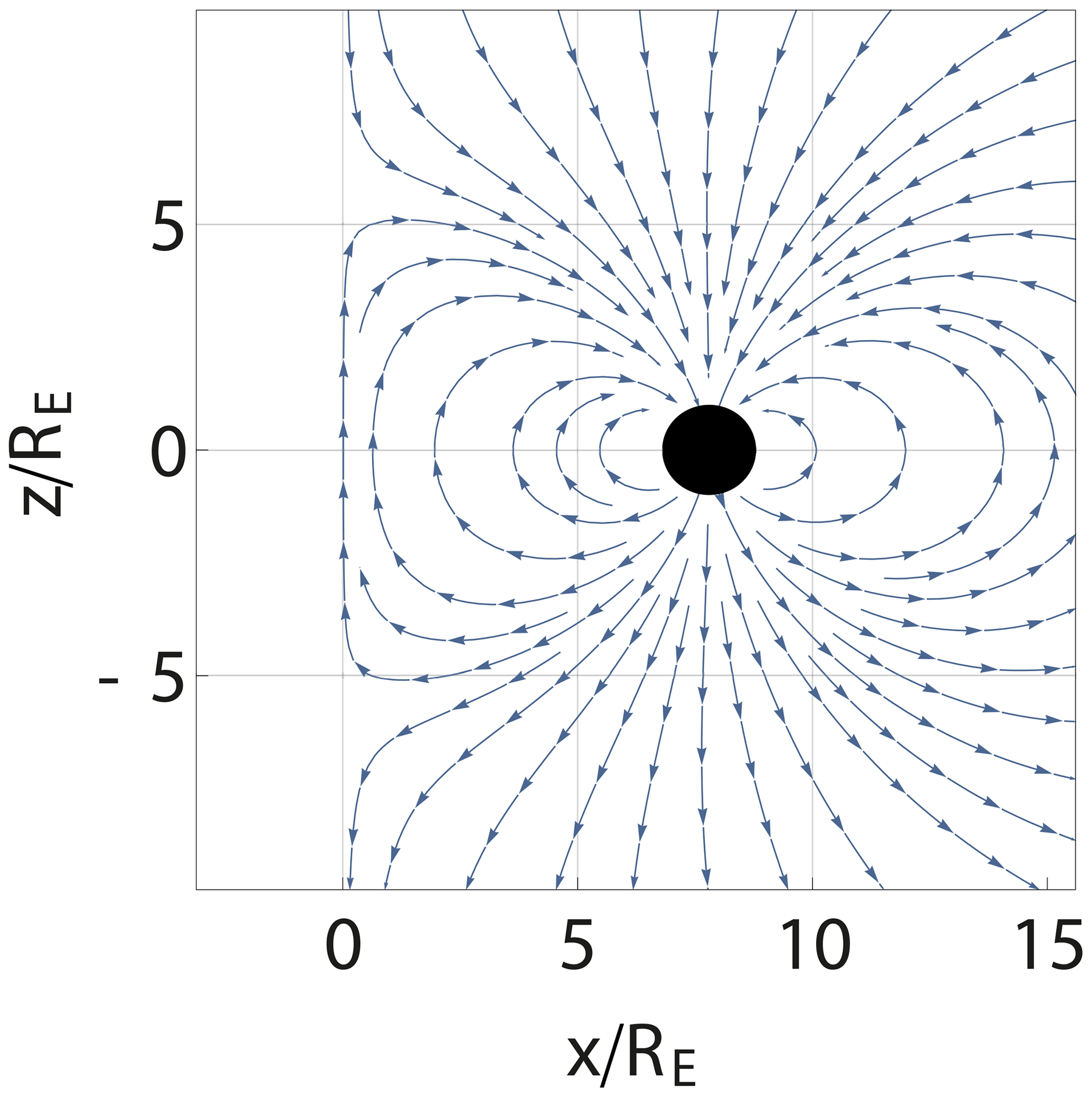
Figure 1Illustration of a cut in a model magnetosphere assuming a plane interface between the Earth's magnetic dipole field and an ideally conducting solar wind. Distances are normalised by the Earth's radius, RE. In this and related following figures, the sun is in the negative x direction so that x is positive in the direction of shock propagation. The stagnation point of the solar wind is taken at . The case illustrated here assumes a strong compression of the magnetosphere by a solar wind pressure pulse by taking the distance to the magnetopause to be 7.8 RE. This value has relevance for data to be shown later. Note the formation of two cusp points.
As the impulse from an ICME shock event arrives at the vicinity of the stagnation point of the solar wind at the magnetopause, its perturbation propagates along the magnetosphere with velocity, depending on the direction with respect to the magnetic field or the magnetopause. As an order of magnitude we can use the following:
where is the Alfvén speed for a plasma mass density ρ and c the speed of light in vacuum. For vacuum or dilute plasmas, we have ϑ≈c, for dense plasmas, ϑ≈VA. We assume the velocity ϑ to be sufficiently large to allow the motion of the magnetopause at all relevant points to be assumed nearly instantaneous for the present problem.
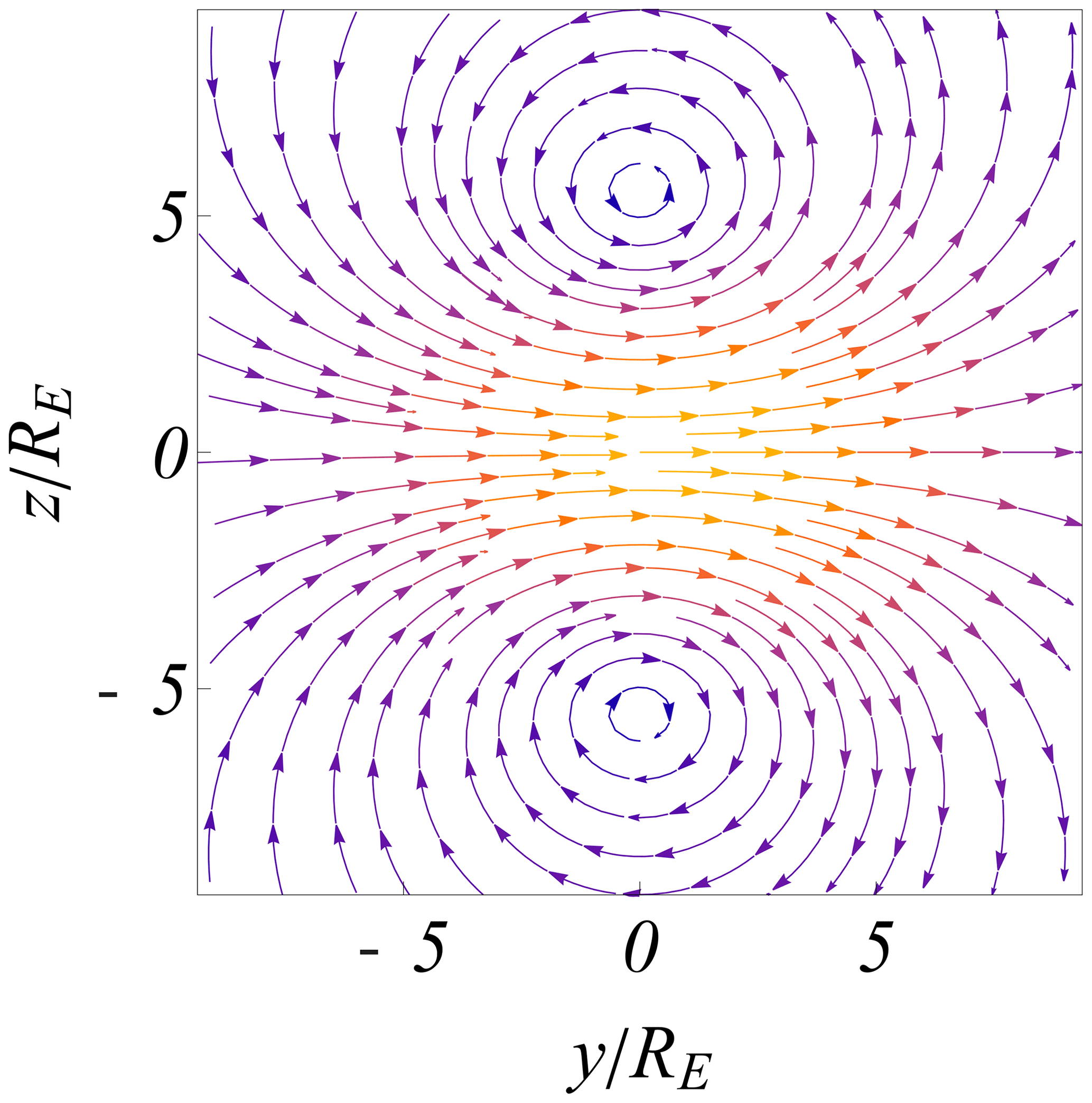
Figure 2The surface current on the interface between the near-Earth's magnetosphere and the solar wind, consistent with Fig. 1. Note the current loops circling the two cusp points. At the Equator, the current is directed from dawn to dusk, as obtained by the magnetic field boundary conditions in Fig. 1.
In its original form, the basic model (Børve et al., 2011) assumed a plane interface between the solar wind and the near-Earth's magnetosphere. An equilibrium state is found when the solar wind ram pressure balances the magnetic field pressure at the stagnation point of the solar wind flow as argued by Chapman and Bartels (1940) and Alfvén (1950). Implicit in the argument is that this ram pressure dominates the electron and ion thermal pressures. The solar wind gives up all its parallel momentum as in an inelastic collision and flows with a reduced velocity along the interface, i.e. the magnetopause, in a boundary layer with an otherwise unspecified thickness and plasma density. The model predicts static parameters such as the distance between the Earth and the magnetopause (stand-off distance), as well as some dynamic features, in particular the frequency and damping of magnetospheric oscillations in response to an impulsive perturbation in the solar wind. For describing the Earth's magnetic field we here ignore the small tilt of the magnetic axis with respect to the rotation axis. For generalising the model to other planets, it is straightforward to include such a tilt of the magnetic axis (Børve et al., 2011). The model can be generalised as shown in Appendices A and B. These changes will, however, only have small consequences for the results. In the following sections we use the simplest version of the model.
2.1 Static limit
For the present formulation of the problem, the total magnetic field resulting from the Earth's dipole and the Chapman–Ferraro current can be found by a simple method of images with details as well as figures presented by Børve et al. (2011). The spatial variations of the magnetic field in the near-Earth's magnetosphere predicted by the model are illustrated here in Fig. 1. In particular, the model predicts the distance from the Earth to the stagnation point of the solar wind. The analysis can be generalised to account for the curvature of the magnetosheath in the vicinity of the stagnation point as well, see Appendix A. The surface currents consistent with Fig. 1 are shown in Fig. 2. Near the stagnation point at the magnetic Equator, the radius of curvature κ increases and ∇B decreases as compared to the value for a magnetic dipole field in free space.
The equilibrium position R for the stand-off distance from the Earth to the magnetopause is found (Børve et al., 2011) by equating the magnetic field pressure (Ferraro, 1952) from the Earth's magnetic dipole moment A m2 to the solar wind ram pressure to give the relation in SI units:
where H m−1 is the permeability of free space, and is the mass density of the solar wind in terms of number density n and average ion mass . The mass density of the solar wind is distinguished from the magnetopause mass density ρ. The contribution to the pressure from the weak solar wind magnetic field is assumed to be negligible. A numerical coefficient in Eq. (1) is a result of the analysis and not a free adjustable parameter. Expressions similar to Eq. (1) can be found in the literature (Walker and Russell, 1995). The scaling with the solar wind dynamic pressure is generally accepted (Southwood and Kivelson, 1990). In fact, apart from a numerical factor, it can be derived from basic dimensional reasoning as shown in Appendix C. The predictions of the model for the distance from the Earth to the magnetopause are shown in Fig. 3 for later reference.
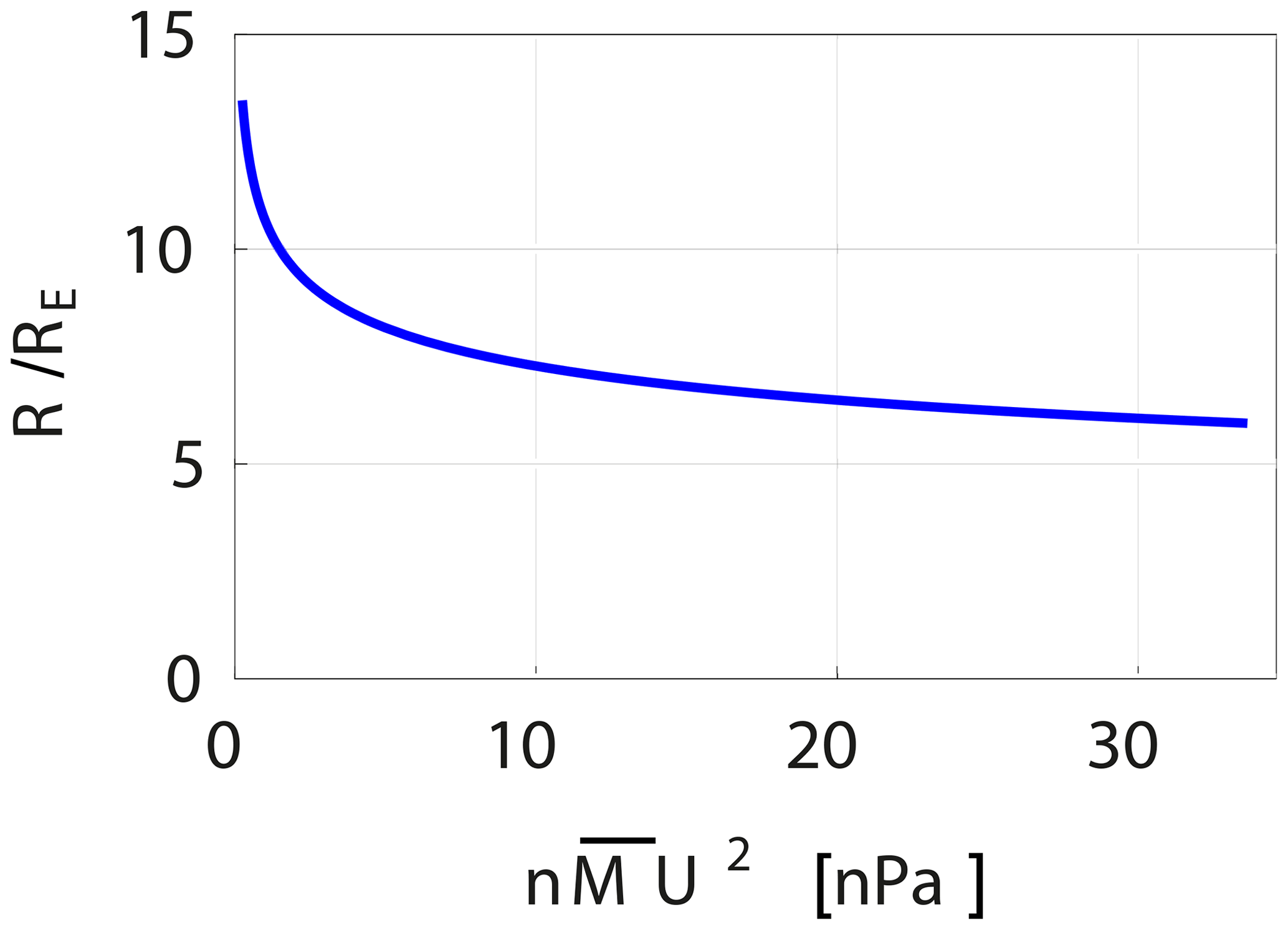
Figure 3The figure shows model predictions for the stand-off distance from the Earth to the magnetopause (Chapman and Bartels, 1940). The distance is measured in units of the Earth's radius RE shown for the varying momentum flux density (expressed in nPa) in the solar wind.
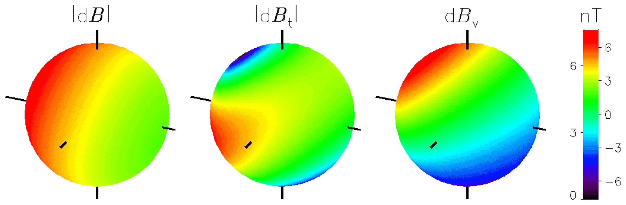
The surface current that models the Chapman–Ferraro current at the interface between the Earth's magnetosphere and the solar wind at x=0 in Fig. 1 induces a small correction to the magnetic field at the surface of the Earth. A change of the stand-off distance R in Fig. 3 will give rise to a change in this correction as illustrated in Fig. 4. The illustration assumes a change from a distance of 11 RE to a new steady state at 7.8 RE. The three spheres show the following: the absolute value of the change in magnetic field, the absolute value of the change in the horizontal magnetic field component, and finally the change in the normal component with respect to the Earth's surface. The latter case is shown including its sign, using the right-hand side of the colour bar. Following the standard convention, we have positive values of the vertical magnetic field component Bv pointing into the Earth. The two other cases have units to the left of the colour bar. We also use this example to illustrate the effects of a tilt of the magnetic dipole axis, see Fig. 5. In cases relevant for the Earth, we find this modification to be of little consequence, and it is ignored in the following section. The results shown in Figs. 4 and 5 refer to vacuum fields without including effects of currents in the Earth's near ionosphere.
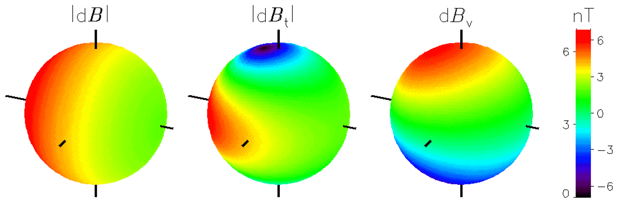
Figure 4Illustration of the change in the magnetic field dB in nT (nanotesla) at the surface of the Earth in response to a change in the distance between the Chapman–Ferraro current and the Earth. In this case, the magnetopause moves from a distance of 11 RE to 7.8 RE. The sun is to the left with the direction given by a small pointer, used also to give the north–south and east–west directions. The direction of the vertical magnetic field component is positive into the Earth. The three figures show , the absolute value of the tangential component (left-hand side of the colour code), and the vertical component dBV (right-hand side of the colour code), respectively. The change in dBV is largest near the magnetic poles.
2.2 Dynamic features
In response to an impulse change in the solar wind ram pressure, the near-Earth's magnetosphere is set into motion. The model of Børve et al. (2011) accounts for this by moving the image dipole in the simple plane interface model as well as in its generalisation summarised in Appendix A.
To find oscillating features, a physical system needs inertia or its equivalent (Smit, 1968; Cairns and Grabbe, 1994; Freeman et al., 1995). The model is not able to predict this inertia, and it is quantified here by a thickness D and a mass density ρ which has to be determined by observations (Song et al., 1990; Phan and Paschmann, 1996) or numerical simulations that are also available (Spreiter et al., 1966). Analytical models have also been proposed (Cairns and Grabbe, 1994) for the width D. Both these parameters vary depending on whether the magnetopause is open (so it has high-density solar wind matter inside) or closed. Densities of ρ=5–25 cm−3 are considered to be typical values. To discuss a finite-amplitude nonlinear case, we write Newton's second law for the position of the interface in the following form:
where Δ(t) is the time-varying displacement of the interface from its equilibrium value R from Eq. (1). The left-hand side of Eq. (2) is the product of the mass and the acceleration of a volume element of the moving magnetopause. The first term on the right-hand side is the ram pressure of the solar wind using the relative velocity between the solar wind and the moving interface at any time. The solar wind is assumed to interact with the magnetopause as an inelastic collision. Reflection as in ideal elastic collision does not apply here. The second term on the right-hand side is the counteracting magnetic pressure due to the dipolar magnetic field of the Earth taken at the magnetic Equator. This force is also derived at the position of the moving magnetopause. We take the sign convention so that Δ>0 when the magnetopause boundary moves in the direction of the Earth (this definition differs from the one used by Børve et al., 2011). The equilibrium solution of Eq. (2) with Δ=0 gives Eq. (1).
2.2.1 Oscillation frequencies and damping
If we linearise Eq. (2), we can derive a scaling law for the characteristic oscillation period as
Apart from the numerical factor, this result can also be found by dimensional reasoning, see Appendix C. A small-amplitude damping coefficient can be found as . Large inertia ρD gives a long oscillation period and a reduced damping. This is intuitively reasonable since it reduces the velocity of the magnetopause. In a related study (Smit, 1968), a drag force was introduced “ad hoc”. Here, the damping is caused by an asymmetry in the solar wind ram pressure: when the magnetopause is approaching (i.e. moving away from the Earth), the magnetopause is doing work on the solar wind, while it is opposite in the receding phase. The two cases are not symmetric since the effective solar wind ram pressure depends on the relative velocity between the solar wind and the magnetopause. In the approaching phase, this force is large, while it is smaller in the receding phase. The work done in the two oscillation phases is different. Integrated over an oscillation period , the oscillations lose energy to the solar wind so the net result is a damping of the oscillations. The initial transient time interval is different: here the solar wind pulse or shock arrives at an interface at rest, and the oscillations are initiated to reach full amplitude.
Magnetopause velocities in the range of 10–20 km s−1 along the normal to the magnetopause have been reported (Paschmann et al., 1993; Phan and Paschmann, 1996). The velocities depend on plasma parameters, the magnetic shear, in particular. The larger of the values quoted refers to high shear (Phan and Paschmann, 1996), although it also seems that the observed speeds have a large statistical scatter. Since the magnetopause is accelerated upon impact from the perturbation in the solar wind (Freeman et al., 1995), these values are only representative, i.e. a large velocity is indicating a large acceleration. Here, results refer to the satellite frame which is moving with a velocity much smaller than the magnetopause. Therefore, only large magnetopause velocities can be determined unambiguously.
The analysis using Eq. (2) and its extensions can also readily give the time variations of the velocity as well as the acceleration . These results are not shown here since we have no access to relevant data for magnetopause velocities, nor accelerations, for comparison. Concerning the time variation of the position Z(t), we have for comparison indirect results in terms of oscillations in, for instance, the magnetic fields that are induced by the moving magnetopause and thereby the Chapman–Ferraro current systems.
There are alternative and more complicated mechanisms that can give rise to damping, i.e. field-aligned currents (FACs) that flow into the polar ionosphere and further to the global ionosphere, where the energy is consumed by the Pedersen currents (Kikuchi et al., 2021). The damping suggested in the present study is of a different nature.
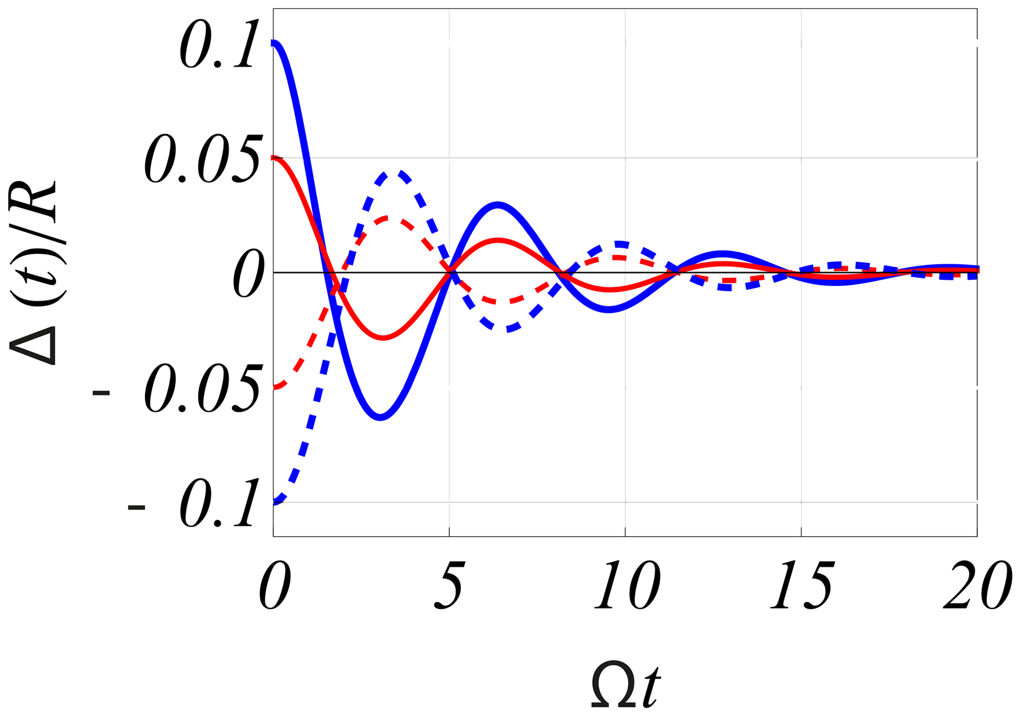
Figure 6Numerical solutions of the nonlinear normalised Eq. (4) for 4 pulse-like initial conditions, Δ(0), two positive corresponding to a compression, and two negative corresponding to rarefaction. Note that the figure is asymmetric with respect to the Δ=0 axis.

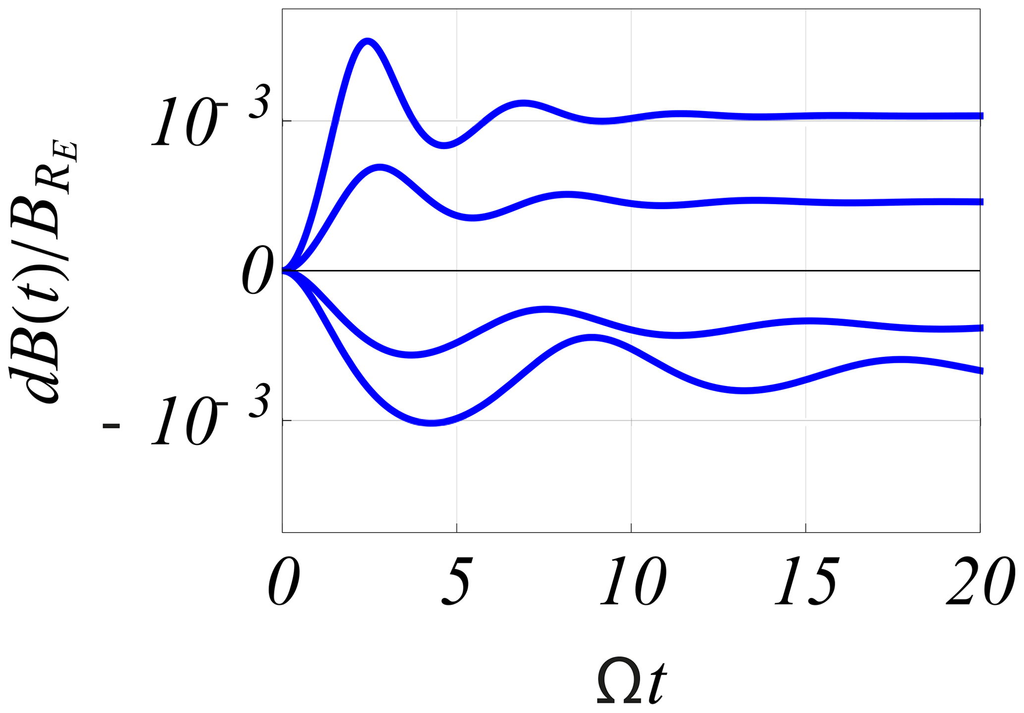
Figure 7Numerical solutions of the normalised Eq. (4). For Δ>0, the solution corresponds to a compression of the magnetosphere in response to a sudden step-like impulse, while Δ<0 corresponds to a sudden expansion.
The basic dynamic Eq. (2) can be rewritten in normalised form (Børve et al., 2011):
with where R is the equilibrium solution Eq. (1), while time is normalised by T0 from Eq. (3). The basic Eq. (4) is strongly nonlinear and the solutions are characterised by significant harmonic generation. Equation (4) can be solved for different conditions, the standard one being where Z is slightly displaced from the equilibrium position to perform damped oscillations, eventually reaching Z=0 as illustrated in Fig. 6. Alternatively, as shown in Fig. 7, we can assume the interface at its equilibrium position until a reference time τ=0, where there is a sudden and lasting change in the solar wind conditions, changing the equilibrium position. The differential equation has to be modified slightly to account for this case (Børve et al., 2011). A relevant problem analysed by the modified version of Eq. (2) corresponds to a sudden step-like change in the solar wind plasma density, which we model here by changing while keeping U constant. The oscillations in Fig. 7 represent transient phenomena occurring between two steady states of the magnetopause, i.e. a time before and one late after the shock arrival. These transient oscillations will modulate those conditions in the Earth's magnetosphere and ionosphere that are induced by changes in the magnetopause.
We estimate the average speed of the magnetopause after it was subject to an impact from a shock-like disturbance in the solar wind by , where its initial position is R0 at time t=0, and the first local maximum of the magnetopause displacement is R1 at t=T0, see Fig. 7. We can write this velocity as by using Eq. (1), where a representative speed is , while the parenthesis is a numerical factor, where comes due to the averaging from the initial time to T0. Realistic values T0≈10 min and give km s−1. This is a large velocity, but it agrees with observations of magnetopause speeds better than an order of magnitude.
The reference calculations in Fig. 7 use , i.e. a relatively large inertia associated with the moving magnetopause. To illustrate the nonlinear character of the oscillations, we show solutions for both positive and negative changes in the solar wind momentum density. For a linear system, the positive and negative parts of Fig. 7 should be mirror images with respect to the horizontal axis. However, we generally expect a different nonlinear response to a sudden increase and a sudden rarefaction in the solar wind. This may also occur, albeit not as often as compression, by a shock. Details of the derivation of the results summarised here are given by Børve et al. (2011), in particular also discussing the simplified linearised limit of the equations.
The physical mechanism causing the damping of the oscillations is found to be an asymmetry in the forcing and the displacement of the magnetospheric boundary. The momentum transfer depends on the solar wind velocity relative to the moving boundary and this is different for an approaching and receding magnetopause. The damping is thus not due to direct dissipation.
2.2.2 Time variations of the magnetic fields
The motion of the Chapman–Ferraro current system induces temporal variations in the magnetic field detected at the surface of the Earth. These are illustrated in Fig. 8. The asymptotic limits t→∞ correspond to Figs. 4 and 5. The analytical expression for the B-field perturbation at the magnetic Equator as found by the use of the image dipole is as follows, using the notation of Figs. 4 and 5:
The nonlinear features of Δ(t) are magnified by the analytical form of dB, the oscillation period depending in particular on the perturbation amplitude as well as its sign. In Fig. 8, we introduce the normalisation, where is the B field at the magnetic Equator at r=RE for t=0; we have a representative value of µT. A characteristic value for the perturbation of the magnetic field deduced from Fig. 8 is thus dB≈30 nT for the given parameters.
The time-varying model magnetic field has a straightforward analytical expression in terms of the moving image dipole. The induced electric field can be derived by Faraday's law, as illustrated here in Fig. 9 for the case where the Chapman–Ferraro current system moves with constant velocity. This is modelled here by moving the image magnetic dipole. Note that a calculation starting from the moving Chapman–Ferraro current system would be complicated, while the result for a moving image dipole is simple. Oscillations in Δ seen in Figs. 6 and 7 give corresponding time variations in the magnetic field. A change in the sign of gives rise to a corresponding change in the sign of the induced electric field in Fig. 9.
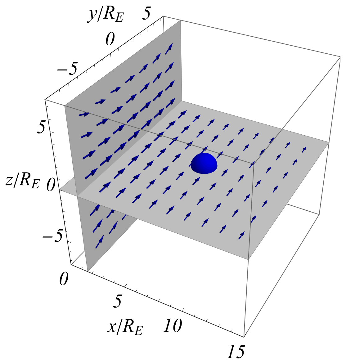
Figure 9Illustration of the electric field induced by the moving Chapman–Ferraro currents, modelled here by an image dipole (as also introduced in Fig. 1), moving with constant velocity. The direction and relative magnitudes of the electric field are shown with blue arrows. The strength of the electric field reduces strongly at large distances on the Earth's nightside. The position and magnitude of the Earth is shown with a blue sphere.
So far, the discussion assumed that the density of matter, plasma in particular, is negligible between the Earth and the magnetopause. Next, we discuss some of the effects on the radiation belts and the Earth's near ionosphere.
2.2.3 Motions of the radiation belts
The moving Chapman–Ferraro current system induces motions of the magnetic field lines (in the magnetohydrodynamic (MHD) sense Pécseli, 2012) in the radiation belts as illustrated in Fig. 10, shown here in the horizontal plane of Fig. 9. Details of individual particle motions are then introduced as corrections to this, e.g. as polarisation drifts. In the analysis we assumed initially quiet conditions with the stagnation point at a large distance from the Earth, see Fig. 1, so that the initial boundary of the radiation belts can be assumed circular. The Chapman–Ferraro current system is then allowed to move the stagnation point from 11 RE to a distance of 7.8 RE from the Earth. We note that the inner boundary is hardly affected since the Earth's magnetic field is too strong there. The deformation of the outer boundary is asymmetric: at the magnetotail side, the electric fields are too weak to induce a motion of any significance (see Fig. 9). On the other hand, the outer boundary on the sunward side is compressed because the magnetic field is relatively weak while the induced electric field has a sufficient magnitude to give a noticeable velocity of the magnetic field line motion. The velocity does not matter for a closed system that is adiabatically compressed: only the initial and final positions of the magnetopause are relevant. For the large magnetopause velocities quoted before (Paschmann et al., 1993; Phan and Paschmann, 1996), we can ignore interactions with the surrounding plasma and use the adiabatic model. The conclusion is that the moving Chapman–Ferraro current system gives rise to an asymmetric compression of the outer radiation belt, which for the given case amounts to approximately 10 %.
The discussion and derivation of the results of Fig. 10 assume that the motion is solely described by the motion of the radiation belts, with the electric field derived from the motion of the Chapman–Ferraro current system. The sudden impulse-like compression of the radiation belts will act as a “piston” and excite compressional Alfvén waves propagating in the Earth's direction. These waves will give rise to a heating of the plasma that will penetrate deeper into the radiation belts (Zong, 2022). The asymmetry of the day- and nightsides will however be well represented by results like those shown in Fig. 10.
The sudden accelerated compression illustrated in Fig. 10 gives rise to polarisation drifts (Chen, 2016; Pécseli, 2012) of the heavy component, here the plasma ions. For the given geometry, the drift velocity is to a first approximation , with time-varying electric and magnetic fields, where Ωci is the local ion cyclotron frequency. At the beginning of the shock compression, the associated currents will be in the dusk–dawn direction as described by Araki (1994), and confined to the compressed region. Strong accelerations during the compression give rise to strong currents. Excess charges will build up at the dawn and dusk boundaries of the compressed regions, see Fig. 11, and these charges can only expand along magnetic field lines or be cancelled by ions or electrons flowing up from the ionosphere along the same magnetic field lines. The polarisation drifts act as generators for these field-aligned currents (FACs) (Araki, 1994). The imposed current density (as modelled by the current generator in Fig. 11) is given as a product of the charge density and the imposed polarisation drift qnUD. The corresponding generator is modelled best by an ideal current generator (Garcia et al., 2015) in contrast to the ideal voltage or potential generator usually assumed for studies of FACs (Knight, 1973) (see also Fig. 11). The ideal current generator has infinite inner impedance, while the voltage generator (ideal battery) has vanishing internal impedance (Scott, 1959). It is known (Garcia et al., 2015) that the distinction has important consequences. Numerical simulations of, for instance, ionospheric double layers (Smith, 1982) demonstrated the importance of the generator impedance. Realistic generator models have finite internal resistances and the two generators are related by the theorems of Thevenin and Norton (Scott, 1959). The potential variations in the circuit, i.e. along magnetic field lines and in the ionosphere, develop in response to the imposed currents. The compression of the radiation belt plasma is modulated by the damped oscillations of the magnetopause. These oscillations in turn modulate the FACs and their time variation will also be recognised in the magnetic fields they give rise to on Earth.
In response to a change in energy density of the ring current, the Dessler–Parker–Sckopke relations (Dessler and Parker, 1959; Sckopke, 1966) predict a detectable perturbation of the magnetic field as measured by e.g. ground-based stations, but these theorems refer to symmetric conditions. The asymmetric perturbation illustrated in Fig. 10 will take some time to relax and thermalise at a rotational symmetry (Summers et al., 2012), i.e. in the order of 4–6 h for a localised distribution of 3 MeV electrons to transform into a uniformly distributed ring. Some details concerning the dynamics of the radiation belts are summarised in Appendix D.
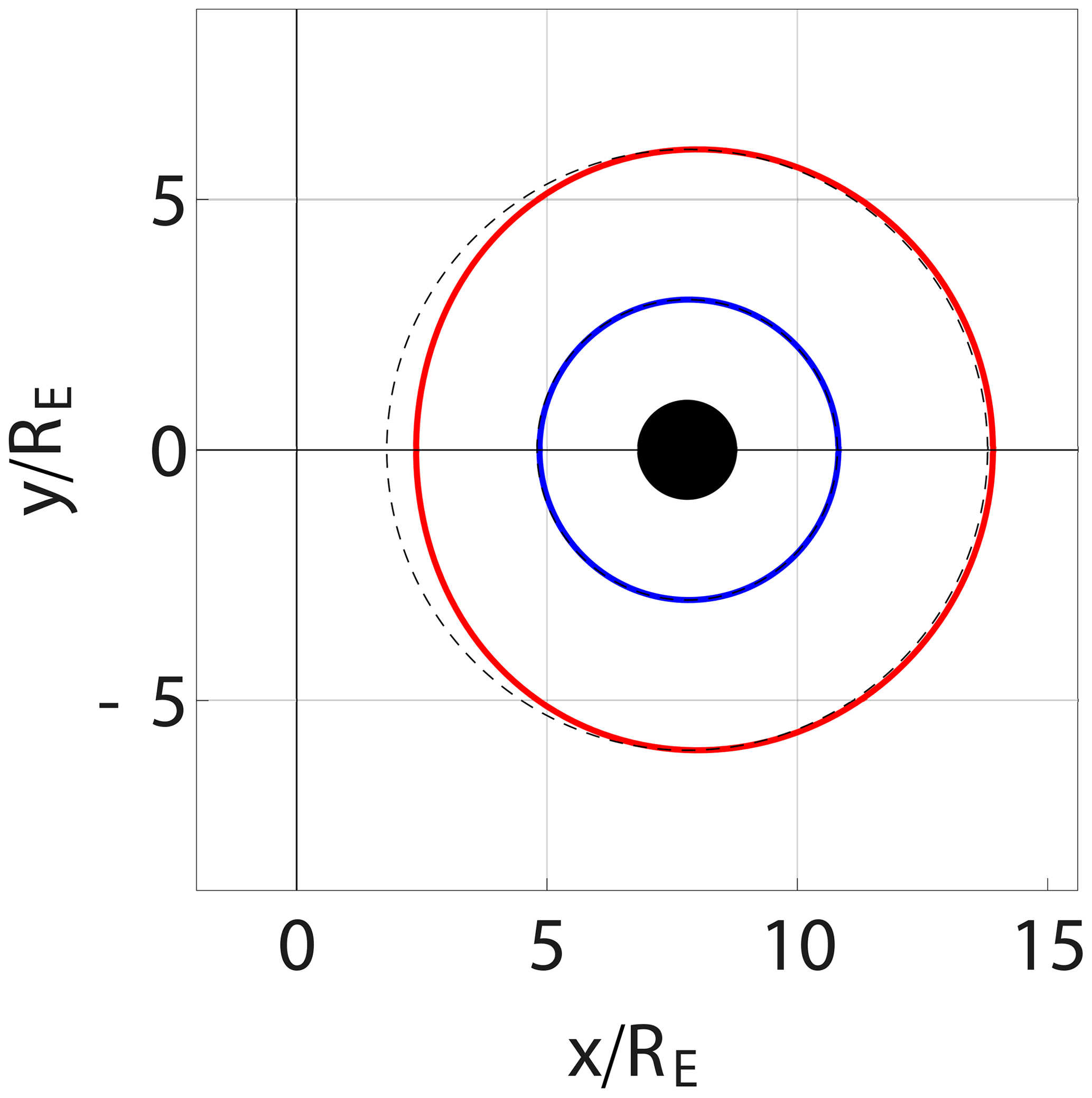
Figure 10Illustration of the compression of the radiation belts induced by the moving Chapman–Ferraro currents. The figure illustrates the displacement of the inner and outer boundaries. The plane of the figure is perpendicular to the Earth's magnetic dipole. Thin dashed lines show the initial inner and outer boundaries, taken here at positions 3 and 6 in units of the Earth's radii RE.
Shock-induced relativistic electron acceleration in the inner magnetosphere have been observed by instruments on spacecraft (Foster et al., 2015; Tsuji et al., 2017). As the radiation belts are compressed in our model, the plasma will be adiabatically heated (Chandrasekhar, 1960) by a transient process. The effect of the heating will depend on the initial energy of the particles in the radiation belt. Charged particles in the MeV range will pass through the compressed region in a time that is negligible compared to the compression time and will not be affected. In our model, the particle energisation is due to the conservation of the magnetic moment (Chandrasekhar, 1960) and therefore a bulk plasma heating, the only constraint being that the plasma particles spend more than a few gyroperiods in the compressed region. For protons, this time will be approximately s, taken at the magnetic Equator at a distance r from the Earth's centre.
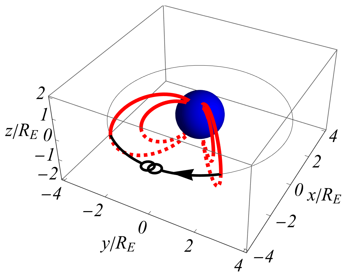
Figure 11Diagram for illustrating polarisation currents (Araki, 1994) generated by an asymmetric compression of the radiation belts, Fig. 10. The current direction is dusk to dawn as indicated by an arrow. Red lines show selected magnetic field lines. The symbol indicates a current generator. The full circuit is discussed by Araki (1994).
The space–time varying electric and magnetic fields generated by the dynamic variations in the position and intensity of the Chapman–Ferraro current system induces currents in the Earth's near ionosphere, the E and F regions. A simple model for idealised conditions is outlined in Appendix B.
The model predictions concerning R and T0, as well as the damping of the oscillations received numerical confirmation (Børve et al., 2011). The agreement was even better than stated by the authors due to an incorrect velocity used for normalisation in the simulations of their Figs. 9, 10 and 13. In reality, the agreement was close to perfect. The numerical model used for the analysis is however in two spatial dimensions, and the steady-state conditions depended on numerical resistivity and viscosity that dominate model viscosity and resistivity (Børve et al., 2014). The importance of viscosity is different for numerical simulations in two and three spatial dimensions. Although this does not affect the dynamic features, a more general test would be worthwhile. Later, fully three-dimensional numerical magnetohydrodynamic (MHD) simulations (Desai et al., 2021) have given more detailed results supporting the restricted solutions found by Børve et al. (2014). There is also a slight difference between the two- and three-dimensional versions of the analytical expressions used in the present work.
The predictions of the model discussed in the previous sections can also be compared to space observations as done in the following section. Here, we distinguish steady-state and dynamic observations.
3.1 Steady-state conditions
Inserting typical numbers as m s−1, m−3, and an average mass equaling the hydrogen mass kg, we find m or R≈11.2 RE in terms of the Earth radius m. The estimates for R are comfortably within the generally accepted range of R∼10–15 RE (Kivelson and Russell, 1995). The model Eq. (1) implies a closed scaling law for the distance to the magnetosheath boundary in terms of the solar wind velocity U and the solar wind mass density . Note that there are no free parameters to fit in Eq. (1), i.e. all are measurable quantities.
3.2 Time-varying conditions
Solar wind disturbances such as interplanetary (IP) shocks induce significant variations of solar wind parameters during a short time interval, introducing perturbations in the geospace environment, particularly sudden variations of the magnetic fields, both in the magnetosphere and on the ground as measured by ground-based magnetometers as well (Araki, 1994; Sun et al., 2015). Fluctuations on the minute timescales are often observed in the magnetosphere in response to strong perturbations in the solar wind. Consistent with a model using nonlinear oscillators (Børve et al., 2011), harmonics of the magnetospheric oscillations are often observed (Kepko and Spence, 2003). These are consistent with the strong nonlinear harmonic generation features of the basic model Eq. (4). Details of other predictions of the model will be compared here with two sets of observations describing responses to shocks in the solar wind. We have chosen two events, 21 December 2014 and 17 March 2015, with significant differences in shock parameters.
3.2.1 Event of 21 December 2014
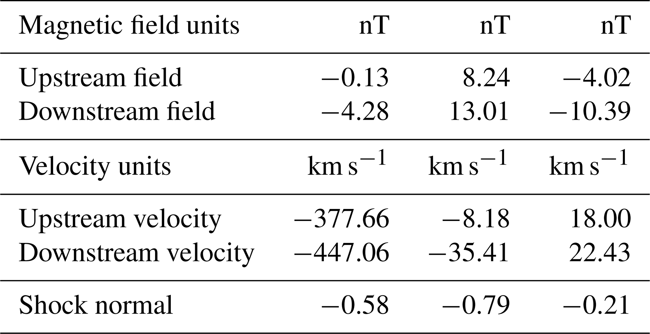
In Fig. 12, we show plasma and magnetic field data from the Wind spacecraft, illustrating the propagation of a shock in the solar wind, seen at ∼ 18:40 UT. Wind is located at RE upstream of Earth. From top to bottom, the plot shows the proton density, bulk speed, temperature, the dynamic pressure, the components of the magnetic field in geocentric solar magnetospheric (GSM) coordinates, and the storm–time (SymH) index. Parameters relevant to the shock are given in Table 1. The shock is driven by an ICME (Richardson and Cane, 2010). The magnetic field upstream of the shock (average over 3 min) is nT, and the shock normal, using the magnetic coplanarity theorem (Colburn and Sonett, 1966) is , both in geocentric solar ecliptic (GSE) coordinates. This gives an angle between the upstream field and the shock normal, , so the shock is quasi-perpendicular. The shock speed is 344.6 km s−1, based on Rankine–Hugoniot relations (see Abraham-Shrauner and Yun (1976) and references therein). The Mach number of the shock is ∼ 4.

Figure 12Data from the Wind satellite showing shock propagation in the solar wind to be compared with the results in the following Fig. 16.
Table 1The shock parameters of event on 21 December 2014. The vector components are expressed in geocentric solar ecliptic (GSE) coordinates.
In Fig. 13, we show data from the CARISMA magnetometer network in Canada (Mann et al., 2008) for a 30 min period. Signals from a few other stations are shown in Fig. 14. An abrupt rise in the magnetic field intensity, followed by some damped oscillations can be seen at about 19:20 UT, where a period in the order of 5–10 min can be noted. The magnitude of the magnetic field perturbations, 10–20 nT, are in reasonable agreement with estimates based on Fig. 8. All signals at the three stations shown start at the same time, although the stations are widely separated spatially. We have considered a larger number of data selected in a band around the Equator and find the same synchronisation of the onset with only a small scatter.
Data from the IMAGE network were also collected, showing somewhat similar results with clear 5 min period oscillations. At the location of the IMAGE stations, the magnetic local time (MLT) at shock arrival is ∼ 22:00 MLT, i.e. pre-midnight. At substorm onset, the stations are prone to the activation of the westward electrojet. In this case, substorm activity was excited by the shock arrival under the prevailing negative interplanetary magnetic field (IMF) Bz conditions (this is seen in the IMAGE magnetograms from the pre-midnight sector; these are not shown here).
The previous Figs. 13 and 14 are local. To give a more global overview, we show the variation of the signal detected by ground-based stations as illustrated in Fig. 15, showing the component normal with respect to ground with a colour code. The radius in the small circles gives the relative variation of the tangential component of the magnetic field perturbation. An intense magnetic field perturbation with a large vertical component and simultaneously small horizontal component will thus be shown with a circle having a small radius. The colour is red if the vertical component is into the ground, and blue if it is in the opposite direction. The stereographic mapping of the globe is chosen to make the circles, having approximately the correct relative magnitudes. When plotting these results, we took the first peak maximum after onset of the signal. Note that in general, the magnitudes of the horizontal components are larger than the vertical components. We find an overall tendency for positive Bz values in the Northern Hemisphere and small or negative Bz values in the Southern Hemisphere. In particular, the variation across Northern America appears uniform. The results are in fair agreement with the model, although not perfect. The strongest deviations are found near the magnetic poles.
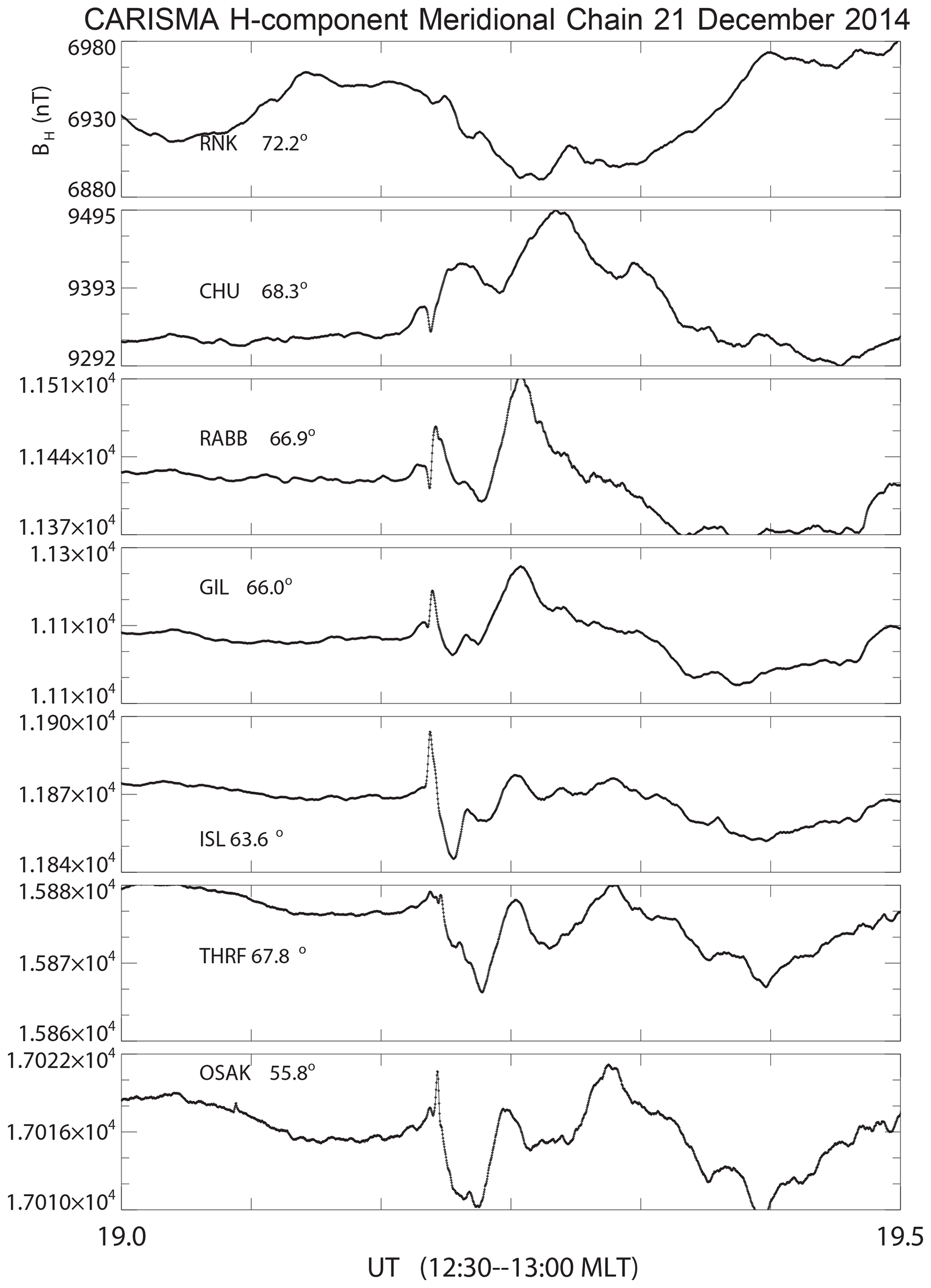
Figure 13Data from the CARISMA magnetometer network in Canada with the stations specified by their acronyms, RNK, CHU, etc. Apart from the top curve, which refers to an open magnetic field line, we see the pulse arrival followed by low frequency, ∼ 5 min period oscillations best seen at corrected geomagnetic (CGM) latitudes 63.6, 67.8 and 55.8∘. The mean values are not subtracted.
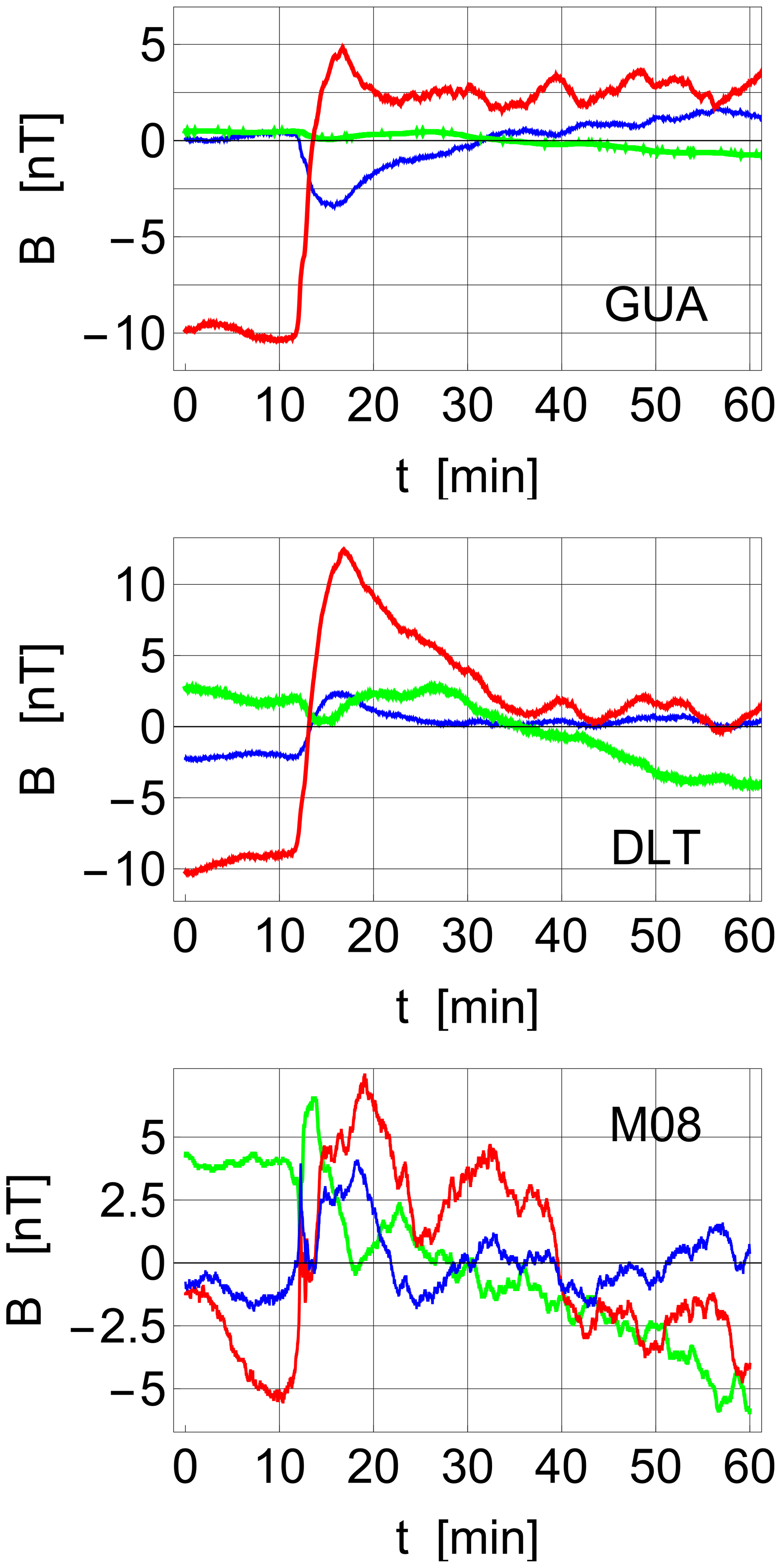
Figure 14Variations of the magnetic field components Bx (red), By (green) and Bz (blue) as observed by the GUA (Guam) and DLT (Dalat, Vietnam) ground stations in response to the shock seen in Fig. 12. Similar data from the M08 (San Antonio) station are shown as well. The averages are subtracted in all figures. The data were obtained by SuperMAG (Gjerloev, 2012). The first data-point is at 21 December 2014, 19:00 UTC. We note some heavily damped oscillations in all figures, where oscillations with 5–10 min periods are discerned.
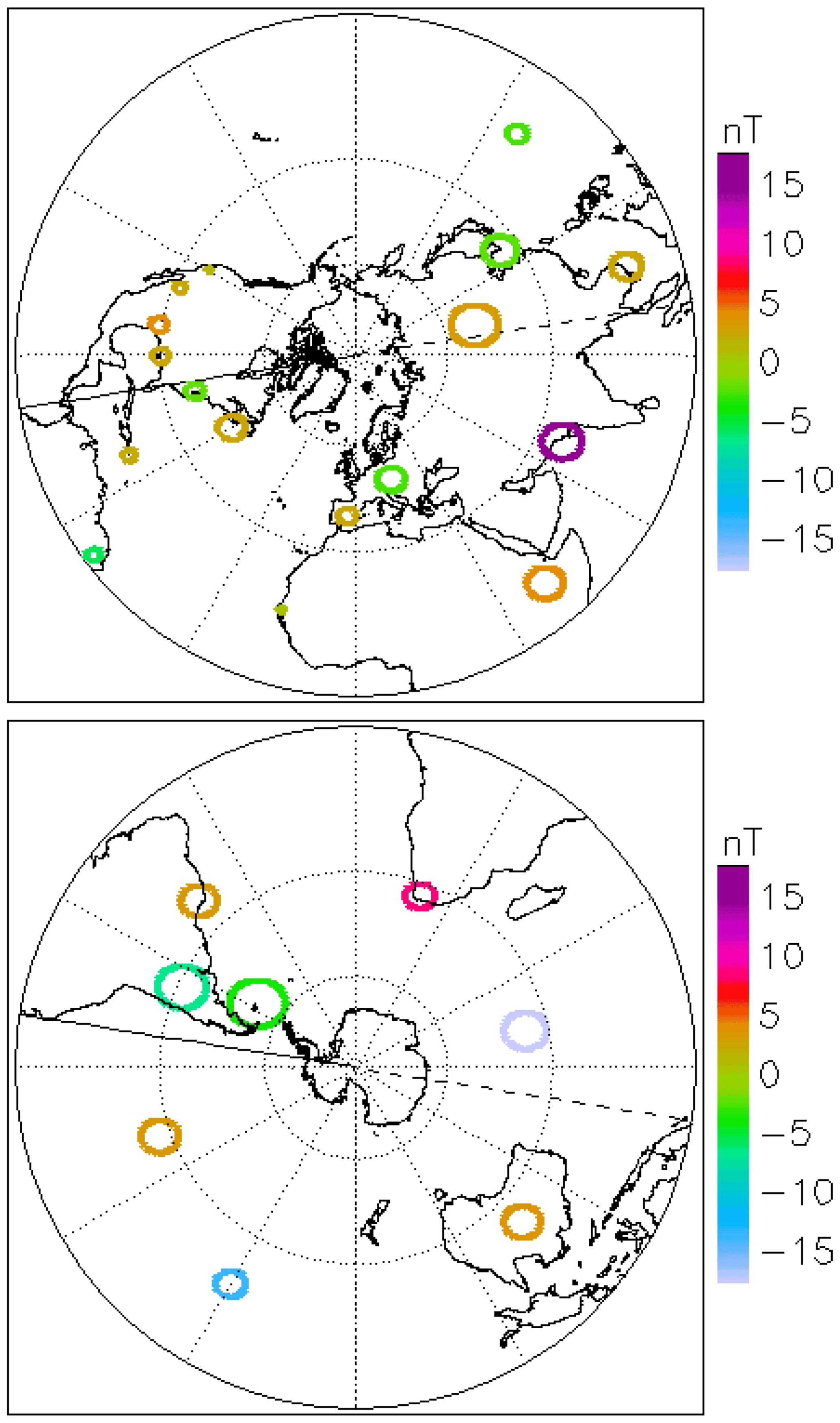
Figure 15Variations of the magnetic field components as detected on ground on 21 December 2014. The data refer to the first peak value after the shock arrival in figures like Fig. 14. North and South America are facing the sun at this time. The data were obtained by SuperMAG (Gjerloev, 2012). The mapping of the circles indicating the horizontal B component follow mapping the continents.
3.2.2 Event of March 17, 2015
In Fig. 16, we show data for 1 d (17 March 2015) from the Wind spacecraft, illustrating the propagation of a shock in the solar wind at ∼ 05:00 UT (see also Table 2). The field and plasma data are analysed in the same manner as the previous shock. The magnetic field upstream of the shock is nT and the shock normal, using the magnetic coplanarity theorem (Colburn and Sonett, 1966) is , with both vectors expressed in GSE coordinates. This gives an angle between the upstream field and the shock normal 115.4∘, so the shock is quasi-perpendicular (). The shock speed is 601.3 km s−1, based on Rankine–Hugoniot relations (see Abraham-Shrauner and Yun (1976) and references therein). The speed of plasma along shock normal is 405.2 km s−1.
In the last panel of Fig. 16, we plot the temporal profile of the SymH index over a 2 d period. The SymH index is a measure of the strength of the ring current. In this case, it has a two-dip structure, indicating that we have a two-dip storm (Kamide et al., 1998). The weaker dip occurs at ∼ 09:15 UT on 17 March 2015. This caused a major storm already. The SymH then recovers for ∼ 14 h, only to decrease again and reach a new and deeper minimum at ∼ 21:00 UT, 17 March 2015. The first dip is caused by the shock compressing Bz<0 (GSM) fields. The second one is caused by the long (∼ 10 h) Bz<0 phase inside the ICME itself. Both strengths correspond to major geomagnetic storms, but the second one almost reaches “superstorm” values (SymH nT). The same thing holds for the event of 21 December 2014, except the SymH dips are much weaker here (∼ 35 and ∼ 60 nT) and they are separated by ∼ 8 h (not shown).
Table 2The shock parameters of event on 17 March 2015. The vectors are expressed in geocentric solar ecliptic (GSE) coordinates.
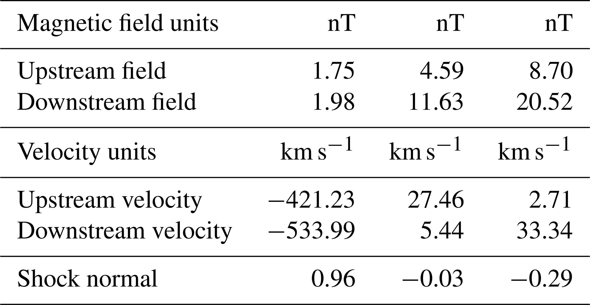
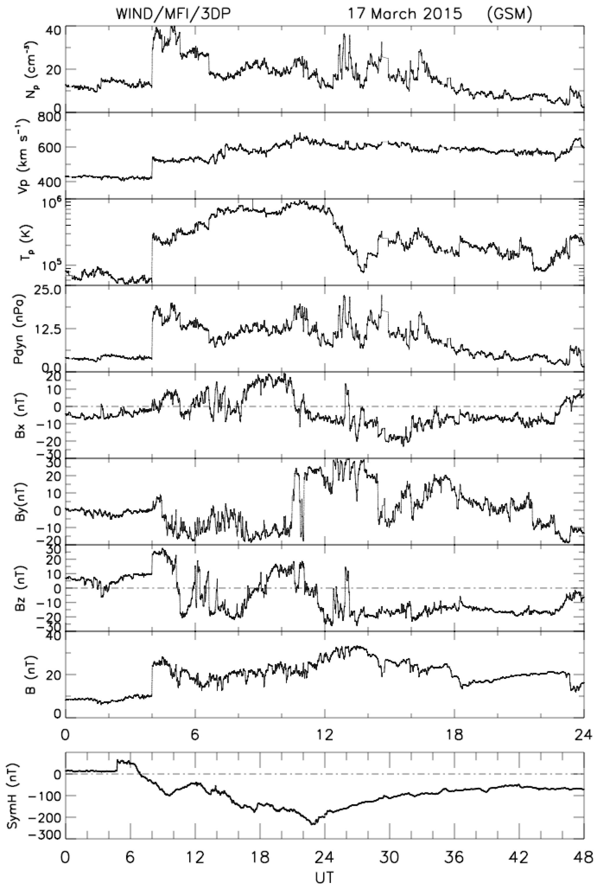
Figure 16The figure shows Wind satellite and ground-based data for the period 17–18 March 2015. The format is the same as Fig. 12, except that the proton beta in the last panel of Fig. 12 is replaced by the storm–time (SymH) index. At ∼ 04:03 UT, a sharp rise is seen in Np, p, Tp, Pdyn and B, indicative of a shock passing the Wind spacecraft. The ground response is recorded ∼ 43 min later with a rise in the SymH index. The configuration resulted in a geomagnetic storm reaching peak values of −234 nT. For completeness and later reference, we show SymH results separately for a duration of 48 h (17–18 March 2015).
At the time of the sudden impulse seen in the SymH index (at 04:46 UT, 5 March) due to the shock seen in Fig. 16, ground stations observed magnetic field variations. Results from the set of the IMAGE magnetometers (Tanskanen, 2009) are shown in Fig. 17. The MLT range of the stations in the UT range plotted is 07:00–09:00 MLT, i.e. they are sampling dawnside local times. Figure 17 shows magnetograms from a wide range of latitudes, extending from the polar cap to middle latitudes. The negative/positive deflections at the northernmost stations on Svalbard (NAL to BJN) are related to the activation of lobe-cell convection under the strongly northward IMF condition at the time of the shock arrival (see Fig. 16).
The bipolar signal seen in our Fig. 17 at auroral latitudes corresponds to the DP-type perturbations (part of the disturbance field of the sudden commencement) described by Araki (1994). The interpretation of this signature given (auroral zone, morning local time) is in terms of an M–I coupling illustrated in Fig. 12 of that work. The described signatures shown in the present work at Svalbard latitudes are explained in terms of lobe-cell polar cap convection with an associated Hall current.
Our focus in the present study is on the impulse/oscillation at lower latitudes during the interval 04:46–04:50 UT, which is more directly related to the IP shock. After a short transition, we see small-amplitude, damped oscillations of 4–6 min periods at 04:46 UT. The signal obtained by selected ground stations at various local times is illustrated in Fig. 18. Here, the MLTs are as follows: at GUA, 14:30 MLT; at DLT, about 12:00 MLT; and at M08 about 22:00 MLT. Note that the vertical scales are larger than those of Fig. 14, consistent with the shock intensity. From Figs. 12 and 16, we estimate the solar wind pressure in the event of 17–18 March 2015 to be approximately twice as large as in the event of 21 December 2014, implying that the characteristic frequency Ω in the former case is larger than in the latter case. The oscillation period is readily estimated visually in Figs. 14 and 18, but the corresponding local frequencies can also be estimated by a wavelet transform (Kaiser, 1994). Illustrative results are shown in Fig. 19. A full wavelet analysis of the signals from a large representative dataset fall outside the scope of the present study, but we note that the wavelets reveal oscillations of 0.5–2 mHz, trailing the step-like magnetic field enhancement that originates from the solar wind shock. This numerical value agrees with our model.
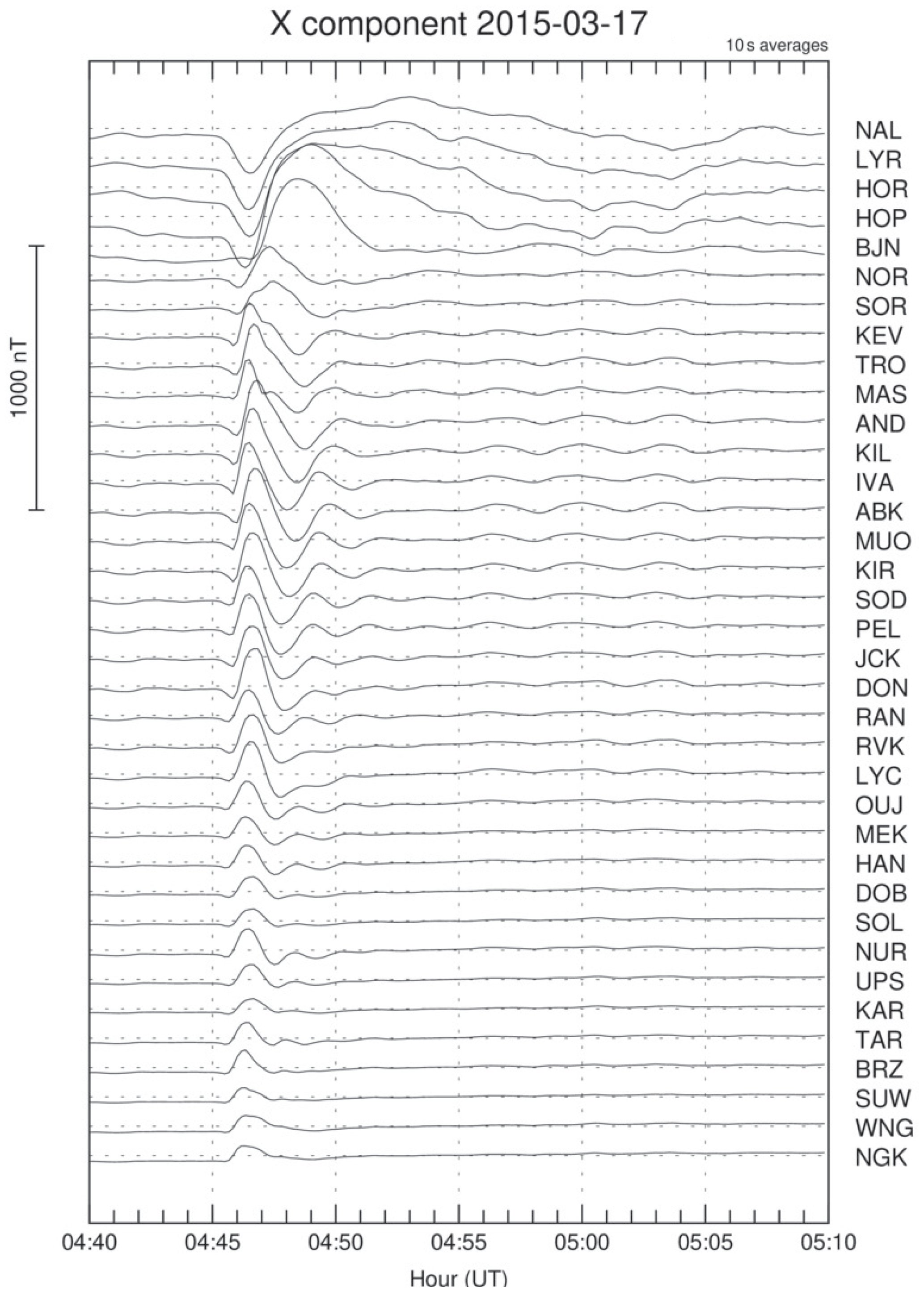
Figure 17X component of the signals detected at the IMAGE stations at the event of 17 March 2015. Each curve is labelled by the acronym for the appropriate station. The data are obtained near 04:46 UT, i.e. around 07:46 MLT (magnetic local time) near dawn. The questions relating to the substorm current wedge mentioned earlier do not apply for this case.
The signal obtained by ground stations at various local times is illustrated in Fig. 20. As in Fig. 15, we show the component normal with respect to ground with a colour code. Positive values point into the Earth here as well. The results near the magnetic poles have magnitudes typically up to 2–3 times larger than the average of the values shown; additionally, the time variations found there can be more irregular. The same comments also apply to Fig. 15 and the values for these regions are not shown. These polar features are believed to be due to FACs (Knight, 1973; Lühr and Kervalishvili, 2021) that are not accounted for in the present model. Ground magnetic disturbances at auroral and subauroral latitudes can be induced by both ionospheric and magnetospheric currents (Araki et al., 1997). At middle and low latitudes, the cause of magnetic field disturbances are dominated by magnetopause currents superimposed by weak ionospheric currents. At the dayside Equator, the ionospheric Cowling currents are the major source for the equatorial sudden commencements (SC). The spatial variations in the magnetic field perturbations seen in Fig. 20 are larger and more non-uniform compared to those found in Fig. 15. We take this as an indication of a stronger influence of the ionospheric currents in the latter case where the solar wind shock is strongest.
For the dynamics in the radiation belts, we have data from the Van Allen Probes (formerly known as the Radiation Belt Storm Probes (RBSP)), with the relevant positions of the two satellites deep inside the magnetosphere shown in Fig. 21. The satellites measure the electric fields as shown in Fig. 22. From Eq. (1), we have m for this case, and from Eq. (3), we find T0≈250 s or approximately 4 min. The magnetopause moves approximately 0.05R within a time , giving a velocity of m s−1 or 60 km s−1 using the estimate from Fig. 7. To represent the temporally changing magnetic field, the image dipole has to move with a velocity U twice this value. The magnetic field from the moving image dipole has to be taken at a distance of approximately 1.5 R from it, i.e. at a position somewhere between the Earth and the magnetopause, giving B≈20 nT. With E≈UB, we estimate E≈2 mV m−1 in the negative direction. This is a value derived for vacuum conditions, while the two probes are located inside the radiation belts, subject to the dielectric plasma shielding. The dominant component of the detected electric field value is in the positive direction (see Fig. 22). We note heavily damped electric field oscillations with approximately 2 min periods. The two satellites (both on the nightside) are at similar distances from the magnetopause and detect similar electric fields. They are however placed at different positions in the radiation belts so the observed particle energy variations are different. In the present context, the electric field measurement acts as a marker for estimating the time delay of the plasma heating pulse.
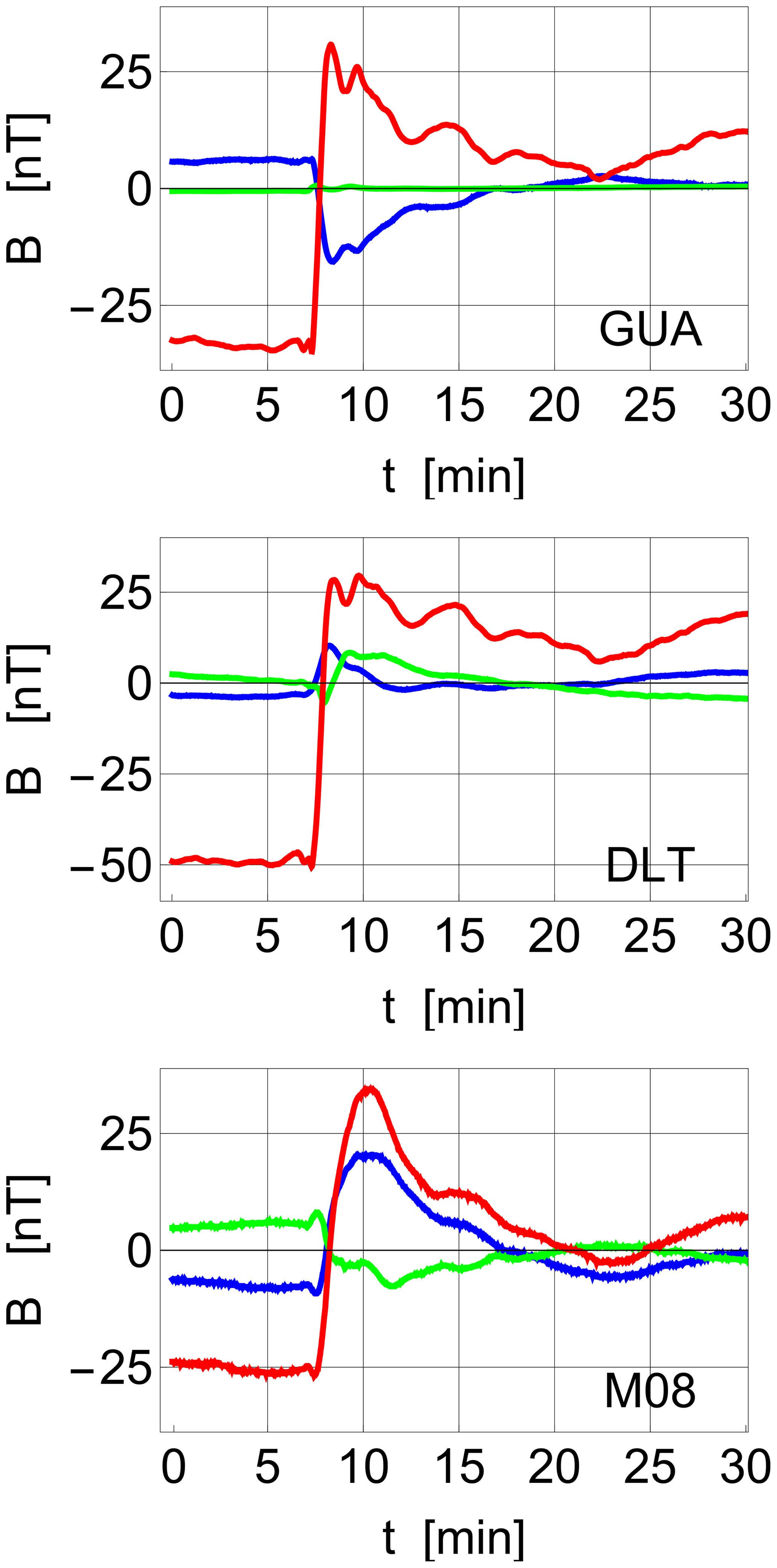
Figure 18Variations of the geomagnetic field components, Bx (red), By (green) and Bz (blue), as observed by ground stations GUA (GUAM), DLT (Dalat) and M08 (San Antonio) in response to the shock seen by Wind (Fig. 16). The magnetic local times (MLTs) being sampled are 04:00 MLT (GUA), 03:00 MLT (DLT) and 12:00 MLT (M08). The averages are subtracted in all figures. The first data-point is on 17 March 2015 at 04:38 UTC. Notice the damped ∼ 5 min period oscillations in the figures. See also Fig. 14 for comparison.
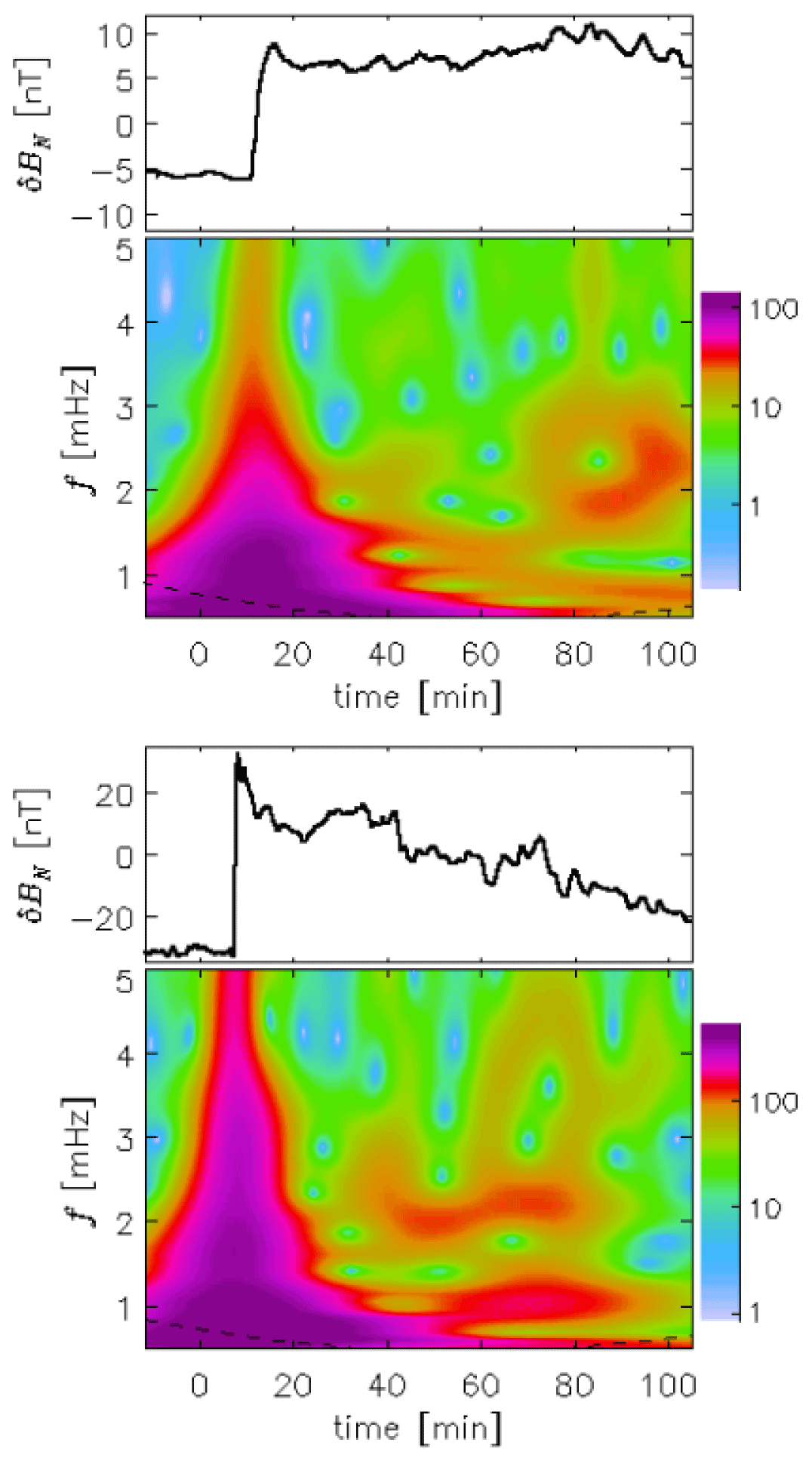
Figure 19Time-frequency representation using a Morelet wavelet for the magnetic X component of the signal from the GUA station (see Figs. 14 and 18 for 21 December 2014 and 17 March 2015, respectively). Note the harmonic content in both samples. The “trumpet-like” form in both figures is the wavelet transform of a step discontinuity originating from the shock impulse. The signals are affected by “edge effects” for frequencies below the dashed line. The results shown here are representative for other stations.

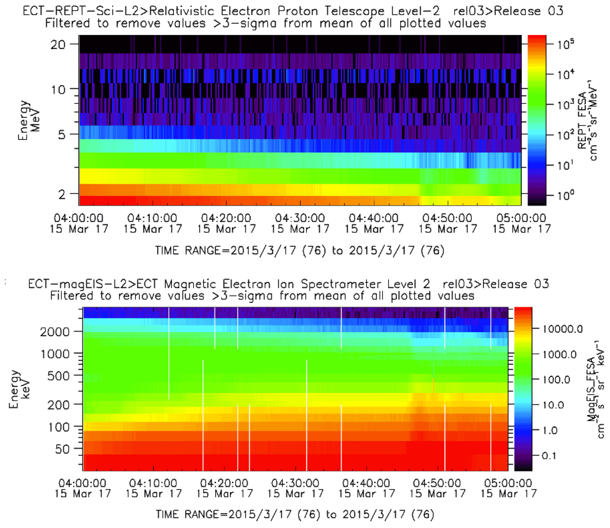
The time variation of the energy distribution of the plasma in the Earth's radiation belt was measured as shown in Figs. 22, 23 and 24. It is the Van Allen Probe A that detects the strongest electron heating in Fig. 22. The REPT (Relativistic Electron Proton Telescope) and MagEIS (Magnetic Electron Ion Spectrometer) instruments (Blake et al., 2013; Baker et al., 2013) on probe B show particle heating at a somewhat smaller level compared to probe A. The heating signal arrives a little earlier (by approximately 1 min) at probe B, see Fig. 21 for the probe positioning. The electrons energised by the compression of the radiation belts as shown in Fig. 10 will have their B×∇B drift in the positive y direction in Fig. 21. These electrons have to propagate to reach satellite A. The estimate in Appendix D is in reasonable agreement with the time delay found in Fig. 22. Due to the compression of the sunward part of the Earth's magnetic field, the estimate of charged particle velocities based on a magnetic dipolar field as in Appendix D will only serve as a guideline.
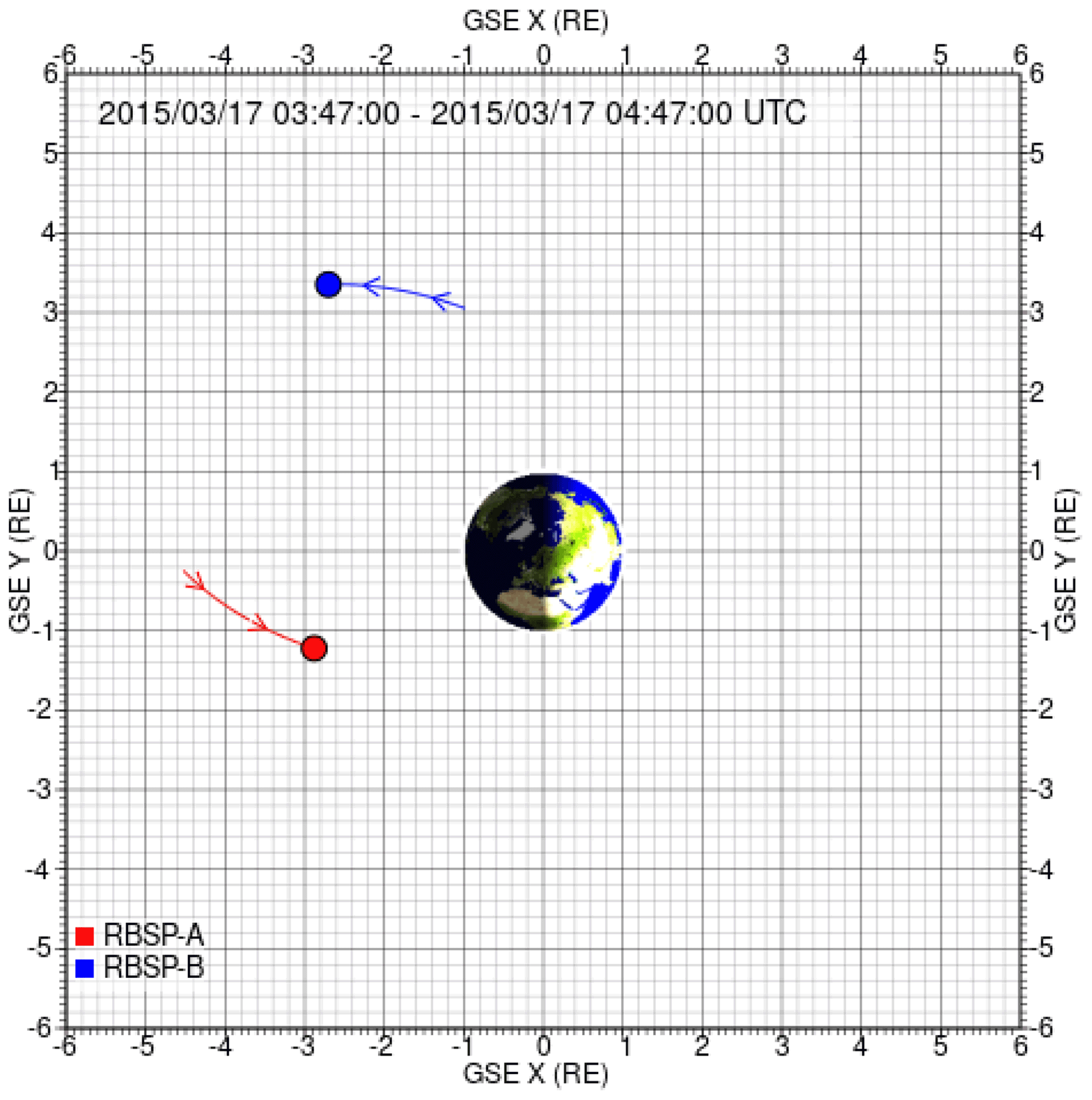
Figure 21Positioning of the two Van Allen satellites with A at approximately the position and B at . The orbits are close to being confined to the x–y plane, so only the projection of the orbits on this plane are shown. The satellite positions are shown at time 04:46 UTC. The duration of the trajectory shown is 1 h. The sun is to the right in this presentation.
A simple model for illustrating the near-Earth magnetospheric static as well as dynamic features has been presented. The model predicts the distance between the Earth and the magnetopause (stand-off distance) without introducing free parameters. Some dynamic features, particularly the frequency of magnetospheric oscillations in response to an impulse in the solar wind is derived as well. The parameter variations of the oscillation frequency is expressed analytically. A damping of the oscillations is predicted, also its variation with solar wind parameters in particular. This damping is not caused by dissipation but is an inherent feature of phase relations in the model. We considered two events for testing the predictions of the model, i.e. two geomagnetic storms: one moderate for 21 December 2014 with SymH nT and a strong one occurring on 17 March 2015 with SymH nT. The magnetospheric response on the impact of them was similar, but with significant differences in the details. The agreement with our model was best for the moderate shock. The magnetic field perturbations in Fig. 18 are significantly larger than those shown in Fig. 14, as expected for the stronger shock. The observed oscillations are consistent with results reported by other studies (Plaschke et al., 2009; Farrugia and Gratton, 2011). Considering the simplicity of our model, we find its overall agreement with observations to be satisfactory. The basic ideas apply for other magnetised planets as well.
The main conclusion of the present study can be summarised in a few words: “Three dipoles suffice for the lowest order modelling of the near-Earth magnetosphere”, one, QE, for the Earth's magnetic field and two image dipoles, where one, QI, is placed in the solar wind and the other, QS, in the Earth's interior (see Appendix B). We have QI and QE to be parallel so their magnetic field contributions add at the Earth's surface. The interior dipole QS is anti-parallel to QE so that the radial component of the magnetic field cancels in the ionosphere at a radius taken here to be RE to sufficient accuracy.
One partial result of the present analysis is an emphasis on the strongly nonlinear features and damping of the magnetospheric oscillations. These are explained here by the basic properties of a simple physical model. The observed frequencies and damping rates seen in, e.g. the CARISMA data in Fig. 13 and in part also the IMAGE data in Fig. 17 are in good agreement with the model results. Ground-based results by SuperMAG are in similarly fair agreement (see Fig. 14 and also Fig. 18). By inspection of Figs. 12 and 16, we find that there are no systematic long-period oscillations of following the shock structure. The oscillations observed in figures like Fig. 13 or Fig. 18 are thus natural for the system and not due to some external forcing. The model also predicts the magnitudes of magnetic and electric fields detected by ground stations and satellites to better than 1 order of magnitude. We consider this to be satisfactory. The ideas put forward in the present study can be applied to any magnetised planet like the Earth, orbiting a star like the sun.
The main limitations of the model are found in the following:
-
It is unable to account for the far magnetotail conditions, the dynamics in particular. A cross-tail current is not included in the model.
-
Magnetic field line reconnection (Califano et al., 2009) is missing in the model. This is important when the interplanetary magnetic field (IMF) has a downward component. Field-aligned currents (FACs) following reconnection are consequently not accounted for.
-
Surface eigenmodes of the dayside magnetopause (Hwang, 2015; Hartinger et al., 2015; Archer et al., 2019) are not accounted for. These will give rise to additional, presumably small-amplitude oscillations to the modes described in our work.
-
The model only gives a schematic account for the excitation of Alfvénic waves and the particle accelerations associated with them.
We believe the present simple model deserves scrutiny. The predictions can be compared to other related data which can be classified according to details such as SymH for the observed shocks.
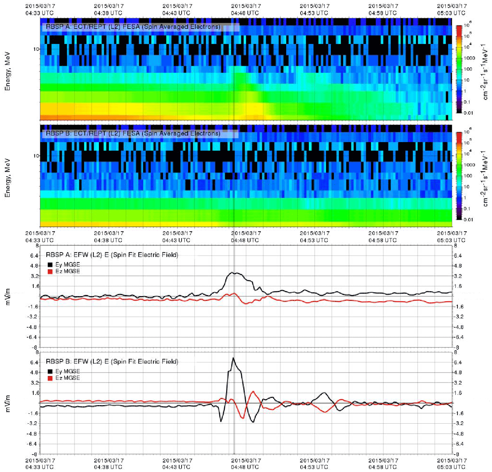
Figure 22Temporal variation of the electron energy distribution (top) and electric field components (bottom) as detected by the two Van Allen Probes. A thin vertical grey reference line indicates the arrival time of the electromagnetic pulse at the Van Allen satellites. Note the time lag of the detected electron heating. The lowest energy particles are delayed most. For 2 MeV particles, the delay is approximately 50 s as found on satellite A. There is only negligible electron energisation detected by satellite B. Strongly damped oscillation in the electric fields have a period of approximately 2 min.
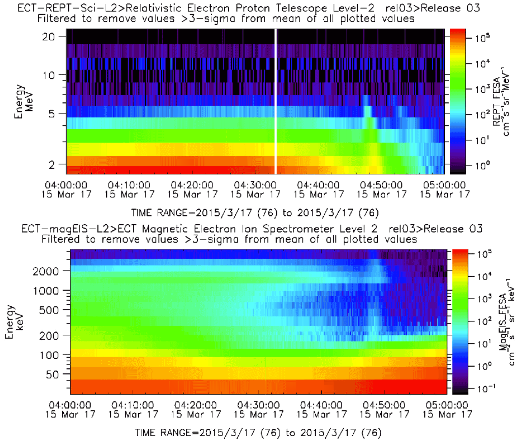
Figure 23Temporal variation of the energy distribution of the plasma particles forming the radiation belts as detected by the Van Allen Probe A. Two energy resolutions of the same event are shown, illustrating that it is the lowest energy particles that are heated most. Note the dispersion in particle velocities: the most energetic particles arrive first, see the top frame. Data from the REPT and MagEIS instruments are shown. The vertical white line is a data gap.
In empty space, we approximate the Earth's magnetic field by a simple dipole, written here in spherical coordinates:
in terms of the angle λ measured from the magnetic Equator. We introduced the magnetic dipole moment Q. For the Earth, we have A m2.
Assume that the cut in interface between the solar wind and the Earth's magnetosphere can be approximated locally by a circle with radius R0, see Fig. A1. The angle between R0 and the line connecting the Earth and the sun is Ψ. At an angular position (r,λ) on the interface, see Fig. A1, we can require (at least for small Ψ, away from the cusp points) an approximate balance in the following form:
Equation (A2) states that the normal component of the solar wind ram pressure balances the magnetic field pressure, keeping in mind that the magnetic field lines are parallel to the curved interface. The magnetic field pressure decreases in the z direction away from the stagnation point, and the component of the solar wind velocity normal to the interface decreases for increasing Ψ as well. The magnetic field on the Earth-ward side of the interface results from the sum of the B fields from the Earth's magnetic dipole Eq. (A1) and an image dipole. Due to the manageable boundary conditions for potentials and electric fields, the method of images is relatively simple for electric point charges, dipoles, etc., in the vicinity of ideally conducting surfaces. For magnetic dipoles, and higher-order multi-poles, the corresponding problems are only simple for some special cases (Ferraro, 1952; Spreiter and Summers, 1965), a plane boundary being one of them.
To obtain an approximation for the magnetic field between the Earth and a curved magnetosphere (Spreiter and Summers, 1965), we take two parallel dipoles here, the Earth's magnetic dipole QE and an image dipole QI at positions xE and xI, respectively. Introducing the magnetic field from a dipole Eq. (A1) and the given radius of curvature for the ideally conducting surface, we find that to the lowest approximation placed on the axis at the position . Near the stagnation point, the total magnetic field becomes
a result that can be derived from the related problem for an electric dipole near a conducting sphere. The first term gives the Earth's magnetic field, the second is the image field. With the notation of Fig. A1, we have and . Introducing Eq. (A3) in Eq. (A2), it is convenient to define a characteristic scale having the physical dimension length6. The origin of the coordinate system is not specified but is determined here through R0 and xE. We could choose to place the origin at the Earth, but the analytical expressions will become more complicated, and we would then have to determine R0 as well as the position for the radius of curvature. For the stagnation point (stand-off distance) of the solar wind at , Eq. (A3) with Eq. (A2) gives the relation , in particular. This is consistent with the result of Børve et al. (2011), since R0−xE is the distance between the Earth and the interface between the solar wind and the magnetopause. A plane interface is a good approximation at (R0,0). Given the parameters, we use Eq. (A2) to determine the radius R0 that eliminates the Ψ dependence, at least to the lowest approximation. A stronger solar wind pressure gives a smaller radius of curvature. As the solar wind pressure decreases, i.e. , we have and R0→∞. We find these latter results to be intuitively reasonable. The approximation works best when Ψ is small. We find that the approximate result R0=γxE, where γ≈1.2–1.5 with the given definition of parameters. This gives and . An example of the modified model with a curved interface between the solar wind and the Earth's magnetic field is shown in Fig. A2. The ideal or desired result would have been a parabolic form for the magnetopause. The method of images is, however, not well developed for such problems. We can postulate a solution with a parabolic shape, where the curvature at the stagnation point is given through the previous analysis.
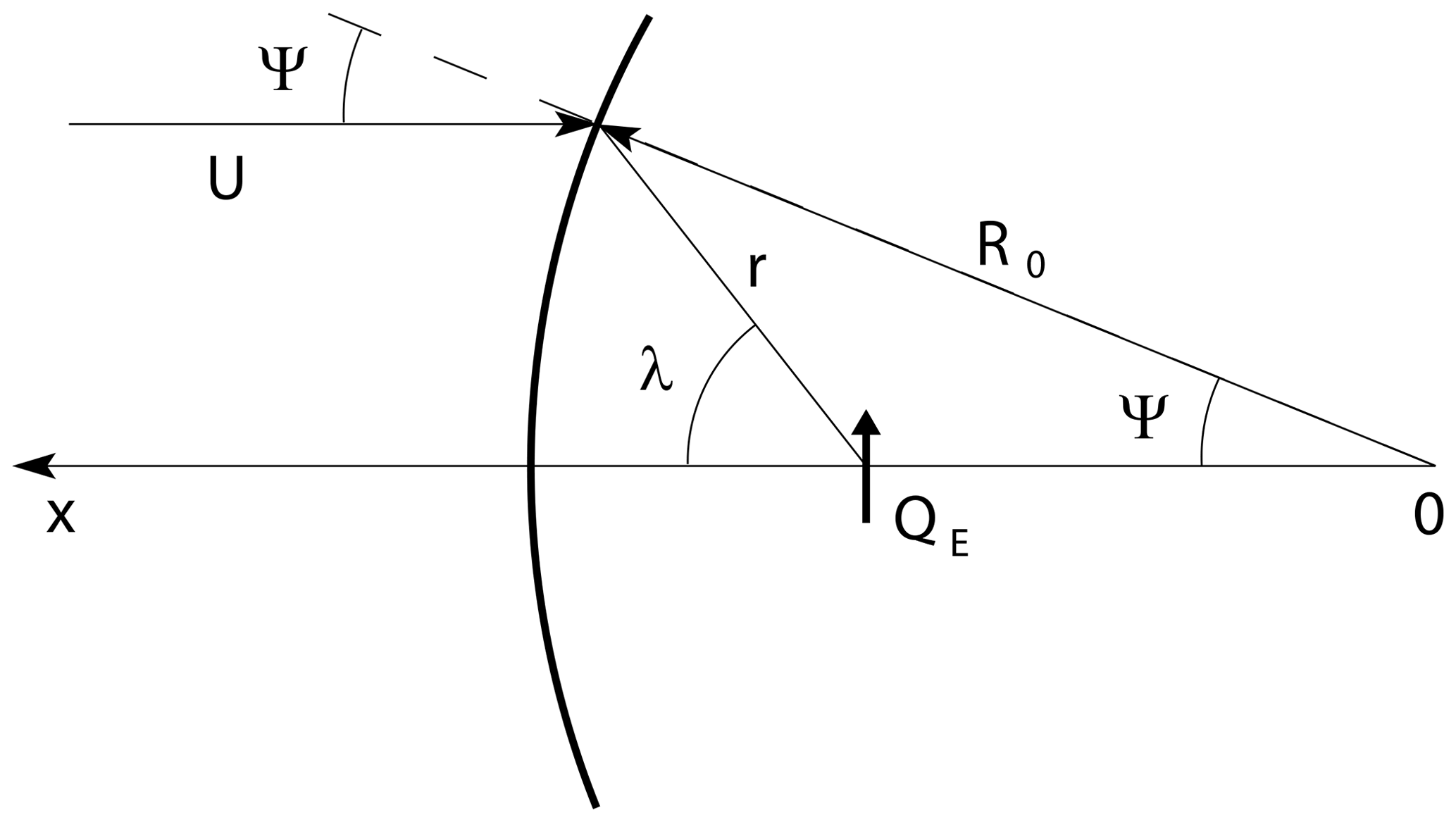
Figure A1Illustration of coordinate system for a modified model of the magnetospheric interface with QE being an equivalent dipole for the Earth's magnetic field. The interface follows the magnetic field lines for small Ψ.
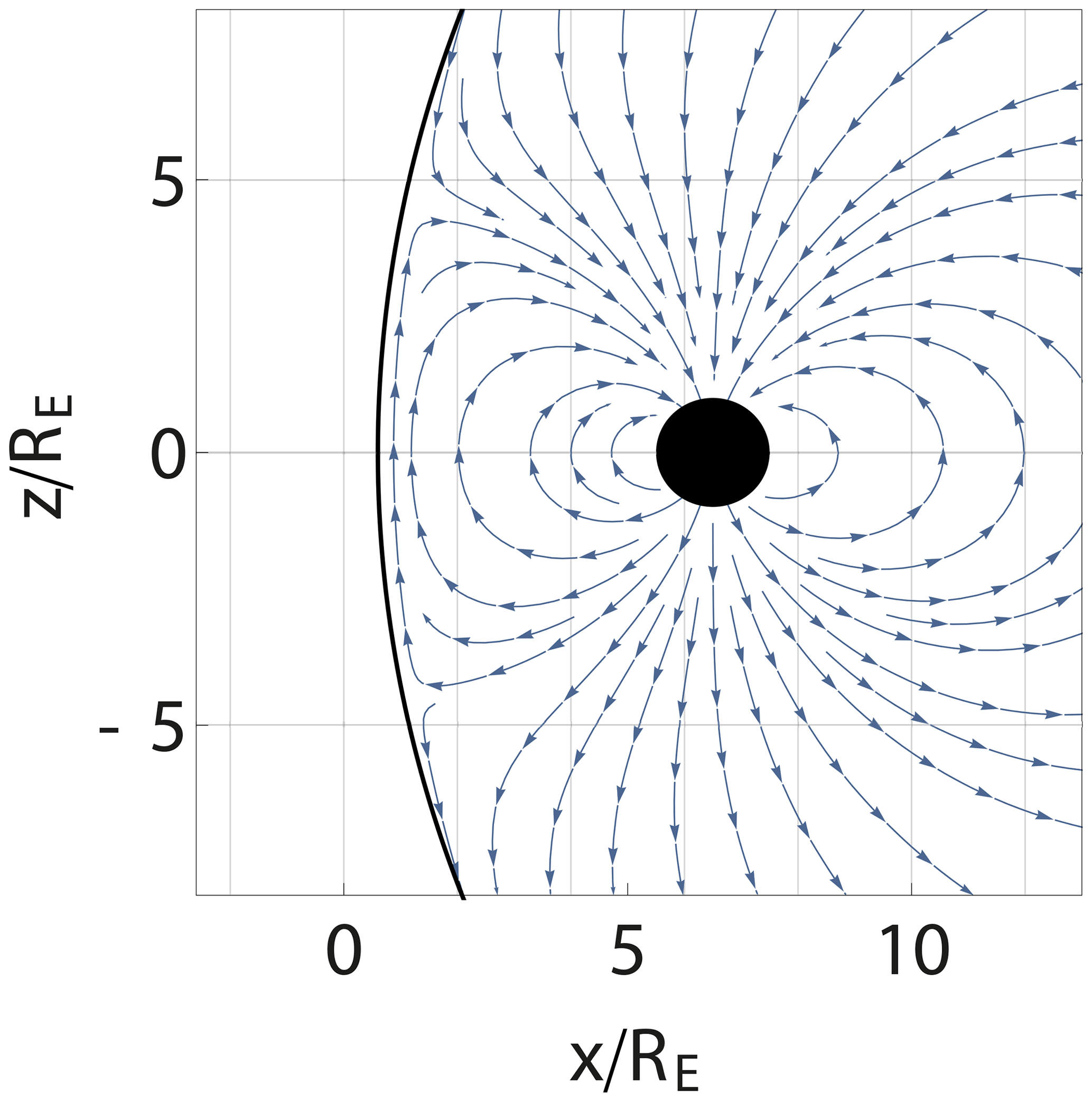
Figure A2Illustration of a generalisation of the results from Fig. 1 where the image method is extended to account for a self-consistent curvature of the interface between the solar wind and the Earth's magnetic field.
An impulse in the solar wind, be it in velocity or density or both, will give rise to a reduction in the distance R0−xE, but at the same time, it will also induce a change in the curvature R0 of the part of the magnetosphere facing the sun. Within the present model, there is no anisotropy in this curvature: it is the same in the plane, parallel and perpendicular to the direction of the Earth's magnetic dipole. The modified model can not account for the formation of the magnetotail.
The space–time varying electric and magnetic fields generated by the dynamic variations in the position and intensity of the Chapman–Ferraro current system induces currents in the Earth's near ionosphere. The ionosphere has a significant altitude variation in the Pedersen and Hall resistivities as well as in the magnetic field-aligned conductivity. The problem can only be solved by strongly idealised conditions, but these can be helpful for giving insight into some general features. For conditions with large plasma parameters, we have a high plasma conductivity ξ, but it will never be super-conducting conditions, so it will be penetrated by a steady magnetic field. For dynamic conditions with large magnetic Reynolds number , where ℒ is a characteristic scale size and U some characteristic velocity, we can assume that the ionosphere acts passively for time-stationary magnetic conditions, but responds as an ideally conducting “shell” to rapid temporal changes in electric and magnetic fields (Davidson, 2001; Pécseli, 2012). This limit has an exact analytical solution when we assume that the moving image dipole field imposes a locally homogeneous time-varying magnetic field at the Earth. In this case, we can formulate the question: “What secondary image dipole is needed to fulfil the boundary conditions at the conducting shell?”, the boundary condition being that the normal component of the magnetic field vanishes at the conducting shell. For the simple limit mentioned before, the answer is readily found. We let be the locally homogeneous magnetic field originating from the moving image dipole at a distance of 2R(t) from the Earth (see Figs. 1 and 3). We now introduce one more image magnetic dipole with dipole moment QS placed at the Earth's centre. For the radial and angular variations of the total magnetic field we have the following:
where it is also most convenient here to measure the angle λ from the Equator of the dipole. With the given choice of polarities, from Eq. (B1), we find that the normal component of the magnetic field at the conducting shell with radius RE vanishes for . At r=RE, from Eq. (B2), we then find the angular magnetic field component Bθ(t)=2BI(t)cos λ. The corresponding surface current density at the bottom of the ionosphere is then in the direction perpendicular to QS in the azimuthal direction ⟂B, thus contributing to the electrojet current. From Fig. 4, we note that the assumption of a locally homogeneous magnetic field imposed by the image dipole representing the Chapman–Ferraro current system can be questioned when the magnetosphere is strongly compressed. In such a case, we can obtain a slight improvement of the previous result by displacing the image dipole QS slightly in the sunward direction. An illustrative result is shown in Fig. B1. An ideally conducting ionosphere would thus shield ground stations completely from temporal variations of the magnetic field. It seems a safe conclusion that a partially conducting ionosphere will reduce the effects of the electric and magnetic field variations as detected on ground. The salty waters of the oceans also act as a conductor, albeit poor in comparison to the ionosphere. The time-varying electric fields will induce currents in the oceans as well, and the resulting (weak) magnetic field variations might be detectable by ground stations.
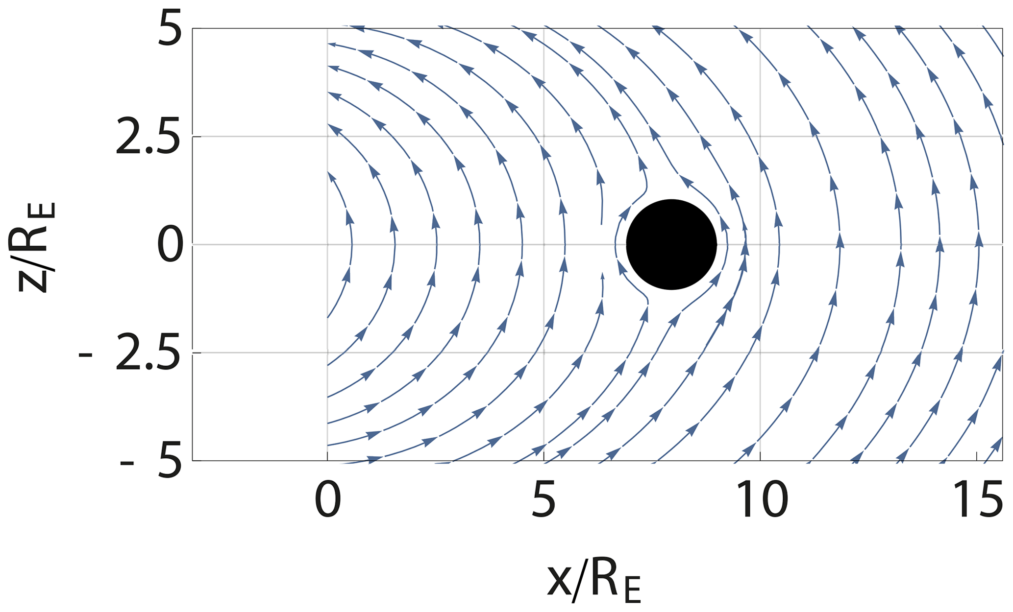
Figure B1Illustration of the change in the magnetic field in the vicinity of the Earth in response to a change in the Chapman–Ferraro current assuming an ideally conducting ionosphere. The figure only shows the time-varying part of the magnetic field: the Earth's steady-state magnetic field is not included.
The time variation of the magnetic field at r>RE follows the variation in BI(t) directly within the given model, see Fig. 8.
Some results can be derived from simple dimensional arguments (Buckingham, 1914). Consider for instance the distance between the Earth and the magnetopause. The basic parameters here are the solar wind ram pressure , where we note that the solar wind density and velocity will always appear in this combination, so there is no generality gained by taking the variables separately. Similarly, μ0 and Q will also appear together, but since μ0 also enters the magnetic pressure, it has to be included explicitly as well. Here, the mass loading will be ρD, where D is the width of the magnetosheath. The dimension matrix for the problem is given by the Table C1.
For a time-stationary problem, where the magnetopause is at rest, we have time T0 in the sixth column to vanish from the problem, and similarly, the inertia term ρD can not have any effect either. Then, the first and third rows are proportional. We write from left to right in terms of the variables on the top in the dimension matrix:
and determine the exponents αj in such a way that the exponents of mass, of time, of length and of current are each equal to zero. Evidently, this requires α1=α4, α2=6α4 and . We arrive at the combination of parameters:
Choosing α4=1, we arrive at the result found in Eq. (1), apart from a numerical constant that can not be recovered by dimensional analysis. Given the parameters entering the problem, the combination in Eq. (1) is thus the only possible one (except a numerical constant) for the stationary problem with the given assumptions. Experimentally verifiable deviations from the scaling will thus indicate that there are missing parameters in Eq. (1). One possibility could be the solar wind resistivity: the magnetic Reynolds number (Davidson, 2001; Pécseli, 2012) is large but still finite so the assumption of ideal conductivity in the application of the method of images can be challenged. We believe that a systematic investigation of this problem is worthwhile.
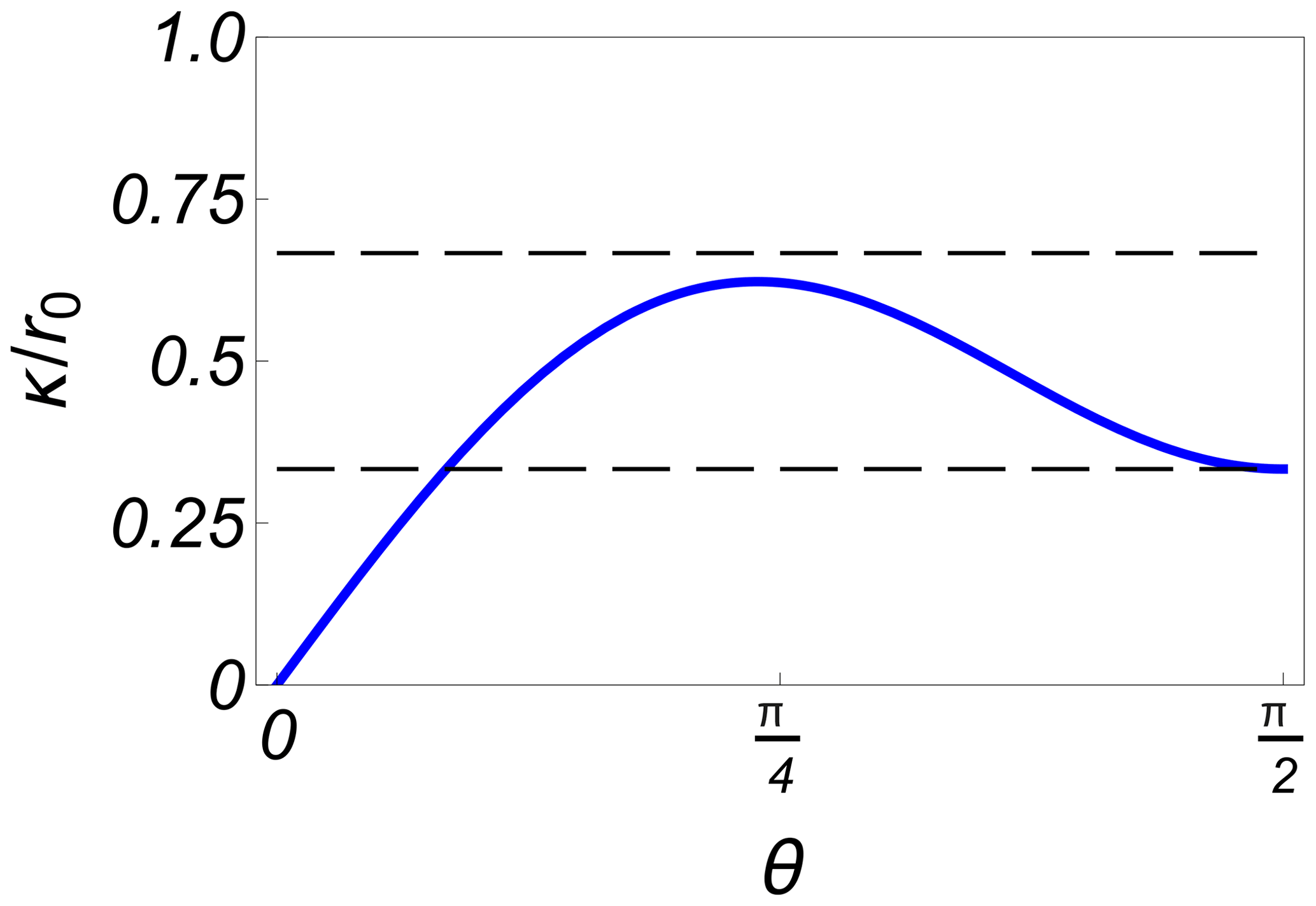
Figure C1The variation of the normalised radius of curvature found as we follow a magnetic field line specified by r0, which is the maximum distance it reaches from the Earth's centre. Two thin dashed lines give and for reference. Here, θ measures the angle from the magnetic pole.
Table C1The dimension matrix for the scaling of the stand-off distance R.

The dynamic problem is somewhat more complicated. Here, we also retain the two last columns in the dimension matrix, and note that any dimensionally correct combination of parameters can be multiplied by the left side of e.g. Eq. (C1), or by to an arbitrary power α0. We can thus decide that some parameters are kept constant, and determine the dimensionally correct combination of the rest. To derive a characteristic period of oscillation T0, we first note that by Newton's second law, Force for the displacement Δ of the magnetopause, we expect the product to appear rather than these quantities individually. As long as the solar wind pressure is kept constant, the variation of the force with varying displacement Δ will be due to the variations of the magnetic pressure with varying distance. We ignore the first column. From the dimension matrix we then have
We find α1=7α4, , α3=α4, giving
Taking α4=1 again, this result is consistent with Eq. (3), apart from a numerical factor.
A damping factor arises by a phase difference between the magnetopause displacement Δ and the velocity , where it is taken into account that the relative velocity between the solar wind and is what matters. A dimensional analysis of this problem will be lengthy.
In this appendix we summarise some details concerning the radiation belt heating due to the asymmetric compression caused by the motion of the Chapman–Ferraro current system. We model the basic averaged gyro-centre velocities by the ∇B drifts:
and curvature drifts (Chen, 2016)
where κ is the radius of curvature for the magnetic field line, also introducing the magnetic moment . With ∇B and κ having opposite directions, the two velocities and add up (Chen, 2016). Using a magnetic dipole as an approximation, we have the expression for a magnetic field line in spherical coordinates as r=r0sin 2θ, where r0 specifies the reference position on the selected magnetic field line as the distance from the dipole centre measured at magnetic Equator, . The radius of curvature can then be found by standard expressions (Pécseli, 2012) as illustrated in Fig. C1. The figure shows the range of validity of Eq. (D2) if we assume κ to be constant.
The time T to circle Earth with the combination of the gradient drift and curvature drifts depends on the selected radius and the particle energy. For a 1 MeV particle at a distance of 5 RE, it takes approximately 103 s, or ∼ 15 min. Combining the velocities in Eqs. (D1) and (D2) to , we have at some distance r from the magnetic dipole centre in the magnetic Equator plane with 𝒲 being the particle energy. Similarly, we have the scaling , implying a particle dispersion in the sense that energetic particles arrive first, see Figs. 22 and 23.
SuperMAG data are available at https://supermag.jhuapl.edu/line; last access: 14 June 2022. INTERMAGNET data are available at https://www.intermagnet.org/data-donnee/download-eng.php; last access: 14 June 2022. The Wind data were downloaded through NASA's cdaweb (Coordinated Data Analysis web) public data centre: https://hpde.io/SMWG/Observatory/Wind; last access: 16 June 2022. All RBSP-ECT data are publicly available at the website https://rbspgway.jhuapl.edu/; last access: 16 June 2022.
All authors contributed to the data collection, analysis and manuscript preparations: HS, PES and CJF mostly to the data collection, HLP and JKT mostly to the analysis and the preparation of the manuscript and figures.
The contact author has declared that none of the authors has any competing interests.
Publisher’s note: Copernicus Publications remains neutral with regard to jurisdictional claims in published maps and institutional affiliations.
Valuable communications with Jesper Gjørlev concerning the use and interpretation of SuperMAG data are gratefully acknowledged. Magnar Gullikstad Johnsen offered valuable comments. One of the authors (HLP) thank Gérard Chanteur for valuable comments. Figure 14 presented in this paper rely on the data collected at the GUA, DLT, and M08 stations. We thank Institut de Physique du Globe de Paris and United States Geological Survey for supporting their operation and INTERMAGNET for promoting high standards of magnetic observatory practice. We thank the institutes who maintain the IMAGE Magnetometer Array and also I. R. Mann, D. K. Milling and the rest of the CARISMA team for data. CARISMA is operated by the University of Alberta, funded by the Canadian Space Agency. Spacecraft Wind data at 3 s resolution were acquired by the Wind Magnetic Field Investigation (MFI; Lepping et al., 1995) and the Wind 3D Plasma Analyzer (3DP; Lin et al., 1995). Data from the Van Allen Probes were accessed at the Science Gateway, maintained by the Johns Hopkins University Applied Physics Laboratory. We thank Bern Blake, Joe Fennell, Seth Claude Pierre, and Drew Turner for use of the MagEIS data and Dan Baker, Shri Kanekal, and Alyson Jaynes for use of the REPT data. Processing and analysis of the HOPE, MagEIS, REPT, or ECT data were supported by the Energetic Particle, Composition, and Thermal Plasma (RBSP-ECT) investigation funded under NASA's Prime contract no. NAS5-01072.
Charles Farrugia was supported by NASA Wind grant nos. 80NSSC19K1293 and 80NSSC20K0197.
This paper was edited by Dalia Buresova and reviewed by Takashi Kikuchi and one anonymous referee.
Abraham-Shrauner, B. and Yun, S. H.: Interplanetary shocks seen by Ames Plasma Probe on Pioneer 6 and 7, J. Geophys. Res., 81, 2097–2102, https://doi.org/10.1029/JA081i013p02097, 1976. a, b
Alfvén, H.: Cosmical Electrodynamics, Oxford University Press, London, ISBN-10: 1541348400, 1950. a, b
Araki, T.: A physical model of the geomagnetic sudden commencement, in: Solar Wind Sources of Magnetospheric Ultra-Low-Frequency Waves, Vol. 81, Geophysical Monograph, The American Geophysical Union, Washington, DC, 183–200, ISBN: 0875900402, 1994. a, b, c, d, e, f, g
Araki, T., Fujitani, S., Emoto, M., Yumoto, K., Shiokawa, K., Ichinose, T., Luehr, H., Orr, D., Milling, D. K., Singer, H., Rostoker, G., Tsunomura, S., Yamada, Y., and Liu, C. F.: Anomalous sudden commencement on March 24, 1991, J. Geophys. Res.-Space, 102, 14075–14086, https://doi.org/10.1029/96JA03637, 1997. a, b, c
Archer, M. O., Horbury, T. S., Eastwood, J. P., Weygand, J. M., and Yeoman, T. K.: Magnetospheric response to magnetosheath pressure pulses: A low-pass filter effect, J. Geophys. Res.-Space, 118, 5454–5466, https://doi.org/10.1002/jgra.50519, 2013. a
Archer, M. O., , Hartinger, M. D., Plaschke, F., and Angelopoulos, V.: Direct observations of a surface eigenmode of the dayside magnetopause, Nat. Commun., 10, 615, https://doi.org/10.1038/s41467-018-08134-5, 2019. a
Baker, D. N., Kanekal, S. G., Hoxie, V. C., Batiste, S., Bolton, M., Li, X., Elkington, S. R., Monk, S., Reukauf, R., Steg, S., Westfall, J., Belting, C., Bolton, B., Braun, D., Cervelli, B., Hubbell, K., Kien, M., Knappmiller, S., Wade, S., Lamprecht, B., Stevens, K., Wallace, J., Yehle, A., Spence, H. E., and Friedel, R.: The Relativistic Electron-Proton Telescope (REPT) Instrument on Board the Radiation Belt Storm Probes (RBSP) Spacecraft: Characterization of Earth's Radiation Belt High-Energy Particle Populations, Space Sci. Rev., 179, 337–381, https://doi.org/10.1007/s11214-012-9950-9, 2013. a
Blake, J. B., Carranza, P. A., Claudepierre, S. G., Clemmons, J. H., Crain, W. R., Dotan, Y., Fennell, J. F., Fuentes, F. H., Galvan, R. M., George, J. S., Henderson, M. G., Lalic, M., Lin, A. Y., Looper, M. D., Mabry, D. J., Mazur, J. E., McCarthy, B., Nguyen, C. Q., O'Brien, T. P., Perez, M. A., Redding, M. T., Roeder, J. L., Salvaggio, D. J., Sorensen, G. A., Spence, H. E., Yi, S., and Zakrzewski, M. P.: The Magnetic Electron Ion Spectrometer (MagEIS) Instruments Aboard the Radiation Belt Storm Probes (RBSP) Spacecraft, Space Sci. Rev., 179, 383–412, https://doi.org/10.1007/s11214-013-9991-8, 2013. a
Blum, L. W., Koval, A., Richardson, I. G., Wilson, L. B., Malaspina, D., Greeley, A., and Jaynes, A. N.: Prompt Response of the Dayside Magnetosphere to Discrete Structures Within the Sheath Region of a Coronal Mass Ejection, Geophys. Res. Lett., 48, e2021GL092700, https://doi.org/10.1029/2021GL092700, 2021. a
Børve, S., Sato, H., Pécseli, H. L., and Trulsen, J. K.: Minute-scale period oscillations of the magnetosphere, Ann. Geophys., 29, 663–671, https://doi.org/10.5194/angeo-29-663-2011, 2011. a, b, c, d, e, f, g, h, i, j, k, l, m
Børve, S., Sato, H., Pécseli, H. L., and Trulsen, J. K.: Low frequency oscillations of the magnetosphere, in: 2014 XXXIth URSI General Assembly and Scientific Symposium (URSI GASS), Beijing, Peoples R China, 16–23 August 2014, IEEE, 1–3, https://doi.org/10.1109/URSIGASS.2014.6929936, 2014. a, b
Buckingham, E.: On physically similar systems; illustrations of the use of dimensional equations, Phys. Rev., 4, 345–376, https://doi.org/10.1103/PhysRev.4.345, 1914. a
Cairns, I. H. and Grabbe, C. L.: Towards an MHD theory for the standoff distance of Earth's bow shock, Geophys. Res. Lett., 21, 2781–2784, https://doi.org/10.1029/94GL02551, 1994. a, b
Califano, F., Faganello, M., Pegoraro, F., and Valentini, F.: Solar wind interaction with the Earth's magnetosphere: the role of reconnection in the presence of a large scale sheared flow, Nonlin. Process. Geophys., 16, 1–10, https://doi.org/10.5194/npg-16-1-2009, 2009. a
Chandrasekhar, S.: Plasma Physics, The University of Chicago Press, Chicago, notes compiled by Trehan, S. K., after a course given by Chandrasekhar, S., ISBN-13: 978-0226100845, 1960. a, b
Chapman, S. and Bartels, J.: Geomagnetism, Vol. 2, Oxford University Press, Oxford, 1940. a, b, c
Chen, F. F.: Introduction to Plasma Physics and Controlled Fusion, Springer, Heidelberg, 3rd Edn., ISBN-10: 9783319223087, 2016. a, b, c
Colburn, D. S. and Sonett, C. P.: Discontinuities in the solar wind, Space Sci. Rev., 5, 439506, https://doi.org/10.1007/BF00240575, 1966. a, b
Davidson, P. A.: An Introduction to Magnetohydrodynamics, 2nd Edn., Cambridge, UK, ISBN: 978-1-107-16016-3, 2001. a, b
Desai, R. T., Freeman, M. P., Eastwood, J. P., Eggington, J. W. B., Archer, M. O., Shprits, Y. Y., Meredith, N. P., Staples, F. A., Rae, I. J., Hietala, H., Mejnertsen, L., Chittenden, J. P., and Horne, R. B.: Interplanetary Shock-Induced Magnetopause Motion: Comparison Between Theory and Global Magnetohydrodynamic Simulations, Geophys. Res. Lett., 48, e2021GL092554, https://doi.org/10.1029/2021GL092554, 2021. a
Dessler, A. J. and Parker, E. N.: Hydromagnetic theory of geomagnetic storms, J. Geophys. Res., 64, 2239–2252, https://doi.org/10.1029/JZ064i012p02239, 1959. a
Farrugia, C. J. and Gratton, F. T.: Aspects of magnetopause/magnetosphere response to interplanetary discontinuities, and features of magnetopause Kelvin-Helmholtz waves, J. Atmos. Sol.-Terr. Phys., 73, 40–51, https://doi.org/10.1016/j.jastp.2009.10.008, 2011. a, b
Ferraro, V. C. A.: On the theory of the first phase of a geomagnetic storm: A new illustrative calculation based on an idealised (plane not cylindrical) model field distribution, J. Geophys. Res., 57, 15–49, https://doi.org/10.1029/JZ057i001p00015, 1952. a, b
Foster, J. C., Wygant, J. R., Hudson, M. K., Boyd, A. J., Baker, D. N., Erickson, P. J., and Spence, H. E.: Shock-induced prompt relativistic electron acceleration in the inner magnetosphere, J. Geophys. Res.-Space, 120, 1661–1674, https://doi.org/10.1002/2014JA020642, 2015. a
Freeman, M. P., Freeman, N. C., and Farrugia, C. J.: A linear perturbation analysis of magnetopause motion in the Newton-Busemann limit, Ann. Geophys., 13, 907–918, https://doi.org/10.1007/s00585-995-0907-0, 1995. a, b
Garcia, O. E., Leer, E., Pécseli, H. L., and Trulsen, J. K.: Magnetic field-aligned plasma currents in gravitational fields, Ann. Geophys., 33, 257–266, https://doi.org/10.5194/angeo-33-257-2015, 2015. a, b
Gjerloev, J. W.: The SuperMAG data processing technique, J. Geophys. Res.-Space, 117, A09213, https://doi.org/10.1029/2012JA017683, 2012. a, b, c
Hartinger, M. D., Plaschke, F., Archer, M. O., Welling, D. T., Moldwin, M. B., and Ridley, A.: The global structure and time evolution of dayside magnetopause surface eigenmodes, Geophys. Res. Lett., 42, 2594–2602, https://doi.org/10.1002/2015GL063623, 2015. a
Hwang, K.-J.: Electron Magnetopause Waves Controlling the Dynamics of Earth’s Magnetosphere: Dynamics and turbulence, J. Astron. Space Sci., 32, 1–11, https://doi.org/10.5140/JASS.2015.32.1.1, 2015. a
Kaiser, G.: A Friendly Guide to Wavelets, Birhäuser, Boston, ISBN: 0817637117, 1994. a
Kamide, Y., Yokoyama, N., Gonzalez, W., Tsurutani, B. T., Daglis, I. A., Brekke, A., and Masuda, S.: Two-step development of geomagnetic storms, J. Geophys. Res.-Space, 103, 6917–6921, https://doi.org/10.1029/97JA03337, 1998. a
Kepko, L. and Spence, H. E.: Observations of discrete, global magnetospheric oscillations directly driven by solar wind density variations, J. Geophys. Res., 108, 1257, https://doi.org/10.1029/2002JA009676, 2003. a
Kikuchi, T., Chum, J., Tomizawa, I., Hashimoto, K. K., Hosokawa, K., Ebihara, Y., Hozumi, K., and Supnithi, P.: Penetration of the electric fields of the geomagnetic sudden commencement over the globe as observed with the HF Doppler sounders and magnetometers, Earth Planet Space, 73, 10, https://doi.org/10.1186/s40623-020-01350-8, 2021. a
Kivelson, M. G. and Russell, C. T. (Eds.): Introduction to Space Physics, Cambridge University Press, UK, ISBN: 0521451043, 1995. a
Kivelson, M. G., Etcheto, J., and Trotignon, J. G.: Global compressional oscillations of the terrestrial magnetosphere – the evidence and a model, J. Geophys. Res., 89, 9851–9856, https://doi.org/10.1029/JA089iA11p09851, 1984. a
Knight, S.: Parallel electric fields, Planet. Space Sci., 21, 741–750, https://doi.org/10.1016/0032-0633(73)90093-7, 1973. a, b
Korotova, G. I. and Sibeck, D. G.: A case study of transit event motion in the magnetosphere and in the ionosphere, J. Geophys. Res., 100, 35–46, https://doi.org/10.1029/94JA02296, 1995. a
Lepping, R. P., Acũna, M. H., Burlaga, L. F., Farrell, W. M., Slavin, J. A., Schatten, K. H., Mariani, F., Ness, N. F., Neubauer, F. M., Whang, Y. C., Byrnes, J. B., Kennon, R. S., Panetta, P. V., Scheifele, J., and Worley, E. M.: The WIND magnetic field investigation, Space Sci. Rev., 71, 207–229, https://doi.org/10.1007/BF00751330, 1995. a
Lin, R. P., Anderson, K. A., Ashford, S., Carlson, C., Curtis, D., Ergun, R., Larson, D., McFadden, J., McCarthy, M., Parks, G. K., Rème, H., Bosqued, J. M., Coutelier, J., Cotin, F., D'Uston, C., Wenzel, K. P., Sanderson, T. R., Henrion, J., Ronnet, J. C., and Paschmann, G.: A three-dimensional plasma and energetic particle investigation for the Wind spacecraft, Space Sci. Rev., 71, 125–153, https://doi.org/10.1007/BF00751328, 1995. a
Lühr, H. and Kervalishvili, G.: Field-Aligned Currents in the Magnetosphere-Ionosphere, Chap. 13, American Geophysical Union (AGU), 195–205, https://doi.org/10.1002/9781119815624.ch13, 2021. a
Mann, I. R., Milling, D. K., Rae, I. J., Ozeke, L. G., Kale, A., Kale, Z. C., Murphy, K. R., Parent, A., Usanova, M., Pahud, D. M., Lee, E.-A., Amalraj, V., Wallis, D. D., Angelopoulos, V., Glassmeier, K.-H., Russell, C. T., Auster, H.-U., and Singer, H. J.: The Upgraded CARISMA Magnetometer Array in the THEMIS era, Space Sci. Rev., 141, 413–451, https://doi.org/10.1007/s11214-008-9457-6, 2008. a
Paschmann, G., Baumjohann, W., Sckopke, N., Phan, T. D., and Lühr, H.: Structure of the dayside magnetopause for low magnetic shear, J. Geophys. Res.-Space, 98, 13409–13422, https://doi.org/10.1029/93JA00646, 1993. a, b
Pécseli, H. L.: Waves and Oscillations in Plasmas, Taylor & Francis, London, ISBN: 978-1-4398-7848-4, 2012. a, b, c, d, e
Phan, T. D. and Paschmann, G.: Low-latitude dayside magnetopause and boundary layer for high magnetic shear: 1. Structure and motion, J. Geophys. Res.-Space, 101, 7801–7815, https://doi.org/10.1029/95JA03752, 1996. a, b, c, d
Plaschke, F., Glassmeier, K.-H., Sibeck, D. G., Auster, H. U., Constantinescu, O. D., Angelopoulos, V., and Magnes, W.: Magnetopause surface oscillation frequencies at different solar wind conditions, Ann. Geophys., 27, 4521–4532, https://doi.org/10.5194/angeo-27-4521-2009, 2009. a, b
Richardson, I. G. and Cane, H. V.: Near-Earth Interplanetary Coronal Mass Ejections During Solar Cycle 23 (199–2009): Catalog and Summary of Properties, Sol. Phys., 264, 189–237, https://doi.org/10.1007/s11207-010-9568-6, 2010. a
Sckopke, N.: A general relation between the energy of trapped particles and the disturbance field near the Earth, J. Geophys. Res., 71, 3125–3130, https://doi.org/10.1029/JZ071i013p03125, 1966. a
Scott, W. T.: The Physics of Electricity and Magnetism, John Wiley & Sons, New York, 1959. a, b
Sibeck, D. G., Baumjohann, W., Elphic, R. C., Fairfield, D. H., Fennell, J. F., Gail, W. B., Lanzerotti, L. J., Lopez, R. E., Lühr, H., Lui, A. T. Y., Maclennan, C. G., Mcentire, R. W., Potemra, T. A., Rosenberg, T. J., and K., T.: The magnetospheric response to 8-minute period strong-amplitude upstream pressure variations, J. Geophys. Res., 94, 2505–2519, https://doi.org/10.1029/JA094iA03p02505, 1989. a
Smit, G. R.: Oscillatory motion of the nose region of the magnetopause, J. Geophys. Res., 73, 4990–4993, https://doi.org/10.1029/JA073i015p04990, 1968. a, b
Smith, R. A.: A Review of Double Layer Simulations, Phys. Scripta, T2/1, 238–251, https://doi.org/10.1088/0031-8949/1982/t2a/031, 1982. a
Song, P., Russell, C. T., Gosling, J. T., Thomsen, M., and Elphic, R. C.: Observations of the density profile in the magnetosheath near the stagnation streamline, Geophys. Res. Lett., 17, 2035–2038, https://doi.org/10.1029/GL017i011p02035, 1990. a
Southwood, D. J. and Kivelson, M. G.: The magnetohydrodynamic response of the magnetospheric cavity to changes in solar wind pressure, J. Geophys. Res.-Space, 95, 2301–2309, https://doi.org/10.1029/JA095iA03p02301, 1990. a
Spreiter, J. R. and Summers, A. L.: Dynamical behaviour of magnetosphere boundary following impact by discontinuity in the solar wind, J. Atmos. Terr. Phys., 27, 359–365, https://doi.org/10.1016/0021-9169(65)90037-1, 1965. a, b
Spreiter, J. R., Summers, A. L., and Alksne, A. Y.: Hydromagnetic flow around the magnetosphere, Planet. Space Sci., 14, 223–250, https://doi.org/10.1016/0032-0633(66)90124-3, 1966. a
Stratton, J. A.: Electromagnetic Theory, McGraw-Hill Book Company, 1941. a
Summers, D., Mann, I. R., Baker, D. N., and Schulz, M. G., eds.: Dynamics of the Earth's Radiation Belts and Inner Magnetosphere, Geophysical Monograph, 199, John Wiley, Washington, DC, ISBN: 978-1-118-70437-0, 2012. a
Sun, T. R., Wang, C., Zhang, J. J., Pilipenko, V. A., Wang, Y., and Wang, J. Y.: The chain response of the magnetospheric and ground magnetic field to interplanetary shocks, J. Geophys. Res.-Space, 120, 157–165, https://doi.org/10.1002/2014JA020754, 2015. a
Tanskanen, E. I.: A comprehensive high-throughput analysis of substorms observed by IMAGE magnetometer network: Years 1993–2003 examined, J. Geophys. Res.-Space, 114, A05204, https://doi.org/10.1029/2008JA013682, 2009. a
Tsuji, H., Ebihara, Y., and Tanaka, T.: Formation of multiple energy dispersion of H+, He+, and O+ ions in the inner magnetosphere in response to interplanetary shock, J. Geophys. Res.-Space, 122, 4387–4397, https://doi.org/10.1002/2016JA023704, 2017. a
Walker, R. J. and Russell, C. T.: Introduction to Space Physics, chap. 6: Solar-wind interactions with magnetized planets, Cambridge University Press, Cambridge, UK, 164–182, ISBN: 0521451043, 1995. a
Zong, Q.: Magnetospheric response to solar wind forcing: ultra-low-frequency wave–particle interaction perspective, Annal. Geophys., 40, 121–150, https://doi.org/10.5194/angeo-40-121-2022, 2022. a
- Abstract
- Introduction
- A simple model
- Comparison with observations
- Conclusions
- Appendix A: Generalisation of the model
- Appendix B: Currents induced in the ionosphere
- Appendix C: Dimensional arguments
- Appendix D: Radiation belt details
- Data availability
- Author contributions
- Competing interests
- Disclaimer
- Acknowledgements
- Financial support
- Review statement
- References