the Creative Commons Attribution 4.0 License.
the Creative Commons Attribution 4.0 License.
 | 20 Jul 2022
Study of the equatorial and low-latitude total electron content response to plasma bubbles during solar cycle 24–25 over the Brazilian region using a Disturbance Ionosphere indeX
Giorgio Arlan Silva Picanço
Clezio Marcos Denardini
Paulo Alexandre Bronzato Nogueira
Laysa Cristina Araujo Resende
Carolina Sousa Carmo
Sony Su Chen
Paulo França Barbosa-Neto
Esmeralda Romero-Hernandez
This work uses the Disturbance Ionosphere indeX (DIX) to evaluate the ionospheric responses to equatorial plasma bubble (EPB) events from 2013 to 2020 over the Brazilian equatorial and low latitudes. We have compared the DIX variations during EPBs to ionosonde and All-Sky Imager data, aiming to evaluate the physical characteristics of these events. Our results show that the DIX was able to detect EPB-related TEC disturbances in terms of their intensity and occurrence times. Thus, the EPB-related DIX responses agreed with the ionosphere behavior before, during, and after the studied cases. Finally, we found that the magnitude of those disturbances followed most of the trends of solar activity, meaning that the EPB-related total electron content variations tend to be higher (lower) in high (low) solar activity.
- Article
(3003 KB) - Full-text XML
-
Supplement
(3782 KB) - BibTeX
- EndNote


The analysis of the total electron content (TEC) is a useful technique for studying the ionosphere responses to several space weather phenomena. Thus, many studies have been conducted that aim to investigate the TEC variations during ionospheric disturbances originating from both external (e.g., magnetic storms) and internal drivers (e.g., gravity waves; Chu et al., 2005; Nogueira et al., 2011; Astafyeva et al., 2015; Figueiredo et al., 2018). In this regard, the TEC is a referential measure of the ionosphere plasma density as a function of free electrons. This parameter can be obtained from the analysis of Global Navigation Satellite System (GNSS) signals and is thoroughly defined as the number of free electrons in the ionized plasma contained along an imaginary tube with a cross section of 1 m2, whose ends are delimited by satellite in orbit and ground receiver (Kersley et al., 2004). Therefore, since the TEC is a good measure of the ionospheric plasma density, many efforts have been made to develop ionospheric indices for quantifying the TEC variations associated with the space weather phenomena (Gulyaeva and Stanislawska, 2008; Sanz et al., 2014; Wilken et al., 2018; Jakowski and Hoque, 2019; Denardini et al., 2020a).
During quiet periods, the ionospheric plasma density tends to follow the regular day-to-day variation in terms of the production/loss of electron–ion pairs, which is controlled mainly by the ratio between solar radiation incidence and the neutral atmosphere density (Kelley, 2009). It is worth mentioning that the term “quiet” has been used to describe both geomagnetic and ionospheric environments within a space weather context (Picanço et al., 2020). In this sense, many space weather phenomena can affect the TEC calculation since it changes the distribution/concentration of plasma in the ionosphere. Among these phenomena are the equatorial plasma bubbles (EPBs), which are plasma irregularities that originate in the equatorial ionosphere under the Rayleigh–Taylor instability (RTI) condition and can propagate to higher latitude ranges (Kelley, 2009; Takahashi et al., 2015). One of the main characteristics of the EPBs is the plasma depletion that occurs in the form of geomagnetic field-aligned irregularities. Thus, the plasma density variation due to EPBs also changes the local ionospheric electrical conductivity, which causes depletion of TEC values due to the ionospheric refraction undergone by the GNSS signals (Otsuka et al., 2002; Takahashi et al., 2016).
Therefore, several ionospheric indices have been developed aiming to measure the ionospheric TEC effects due to EPBs. Among them, the rate of TEC index (ROTI) is a technique for quantifying the amplitude of GNSS phase fluctuations and is commonly used as a direct measure of the EPBs occurrence (Pi et al., 1997; Cherniak et al. 2018; Carrano et al., 2019; Liu et al., 2019a, b; Borries et al., 2020; Carmo et al., 2021). Another widely used index for monitoring the EPB effects is the scintillation index (S4), which represents a value of ionospheric scintillation on GNSS signals mainly in the equatorial and low-latitude regions and is capable of estimating the magnitude of the EPB-related scintillations (Aarons, 1982; Kintner et al., 2007). Furthermore, Denardini et al. (2020a) presented a new version of the Disturbance Ionosphere indeX (DIX), which provides a dimensionless value of the ionosphere perturbation degree during phenomena of both internal and external origin.
The DIX was firstly proposed by Jakowski et al. (2006) as a proxy for the TEC response due to magnetic storms. Later, new versions of this index were introduced that aimed to analyze the phenomena originating from internal and/or external drivers (Jakowski et al., 2012; Wilken et al., 2018; Denardini et al., 2020a). Among them, the DIX version presented by Denardini et al. (2020a) has been used for evaluating ionospheric disturbances over the Brazilian region. Additionally, Picanço et al. (2020) presented a statistical evaluation of the DIX equation that Denardini et al. (2020a) proposed. The authors stated that the new DIX approach proved to be effective in detecting ionospheric disturbances due to internal sources and that the new method for calculating the DIX non-perturbed reference also made the index more sensitive to short-term TEC time variations. Afterward, Picanço et al. (2021) used the same DIX version to provide an analysis of the equatorial and low-latitude ionospheric response to disturbed electric fields during extreme geomagnetic storms over the Brazilian region. Moreover, the authors discussed the DIX response to pre-storm effects and other phenomena, such as sporadic E layers. Denardini et al. (2020b) analyzed DIX maps calculated for South America during extreme geomagnetic storms and plasma bubbles. Besides the magnetic storm analysis, the authors associated local disturbances in DIX with the equatorial spread F (ESF) observed over the same area of study. However, as it was a preliminary study, the authors did not delve into the physical explanation of the DIX responses due to plasma bubbles. In addition, they presented only one EPB case that occurred along with the St. Patrick's Day magnetic storm period.
This study aims to evaluate the equatorial and low-latitude ionospheric responses to several plasma bubble events distributed along the period from 2013 to 2020 over the Brazilian region. Therefore, we used the DIX version presented in Denardini et al. (2020a) to characterize the ionospheric TEC disturbances due to the EPBs and compared it to the occurrence of ESF/plasma irregularities observed on ionosonde and All-Sky Imager OI (atomic oxygen line) 630 nm airglow data. Our results show that the DIX can detect EPB-related TEC disturbances in terms of their intensity and times of beginning and end. In short, the DIX responses were consistent with the ionosphere behavior before, during, and after the occurrence of these phenomena. Finally, we found that the magnitude of TEC disturbances followed the trend of solar activity, which means that the EPB-related TEC disturbances tend to be higher (lower) in high (low) solar activity.
2.1 The Disturbance Ionosphere indeX (DIX)
We used the DIX methodology presented in Denardini et al. (2020a) to analyze the TEC variations during plasma bubble events over the Brazilian equatorial and low-latitude ionospheric regions. In this regard, we calculated the DIX using TEC data obtained from the method presented in Seemala and Valladares (2011). The DIX for a specific GNSS station is defined by Eq. (1), as follows:
where is the difference between the current TEC value and the non-perturbed TEC reference for the k-esime geographic coordinates (k = latitude, longitude), for a given time t. TECk is the current vertical TEC value for the k−esime geographic coordinates, is the non-perturbed TEC reference obtained from a 3 h centered moving average along the reference day for the k-esime geographic coordinates, and α is the value at local midnight, obtained for each period of analysis. Finally, β is a latitude-dependent term used to normalize the DIX value into a scale ranging from 0–5. Thus, it is relevant to mention that the reference day is defined as the geomagnetically quietest day of the period of study, where no depletions greater than 20 TEC units over a 1 h period were observed in the nighttime TEC. More details on the DIX calculation can be found in Denardini et al. (2020a) and Picanço et al. (2020).
The DIX is an index developed for representing the ionosphere perturbation degree during several types of phenomena (e.g., disturbed electric fields, plasma bubbles, and sporadic E layers). Therefore, we highlight that the ionospheric responses observed using this index are generally caused by the sum of concomitant events which can be caused by internal and/or external drives (Denardini et al., 2020a, b; Picanço et al., 2020, 2021). Thus, those studies demonstrate that the current DIX methodology provides a straight response to space weather events in which it is possible to estimate the intensity and duration of ionospheric disturbances.
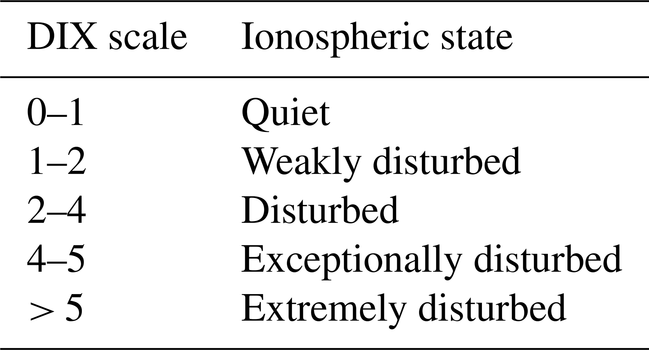
The DIX provides a single and dimensionless value that represents the ionosphere degree of perturbation within a scale of ionospheric states. This scale ranges from 0–5 (Table 1) and represents the intensity of phenomena detected by DIX (Denardini et al., 2020a).
2.2 ROTI calculation
To validate the DIX capability in responding to EPB-related TEC disturbances, we compared it to the ROTI values during selected events. The ROTI is an index proposed by Pi et al. (1997) as an attempt to measure GNSS phase fluctuations, and it is currently one of the most used indices to study plasma bubbles. In this regard, the ROTI derives from the rate of change of TEC (ROT), a parameter that has been widely used to measure the effects of ionospheric irregularities on GNSS signals since the early 1990s (Wanninger, 1993; Doherty et al., 1994; Aarons et al., 1996). Specifically, the ROT represents the GNSS phase fluctuations as a measure of the time rate of a given TEC time series, as shown in Eq. (2) as follows (Pi et al., 1997):
where t is the current time, and represents the TEC at given times, t1 and t2. The ROT is given in the unit of TECUs per minute.
The ROTI is given by the deviation of ROT within a 5 min time interval, as presented in Eq. (3) as follows (Pi et al., 1997; Carmo et al., 2021):
The term 〈ROT〉 in Eq. (3) means the arithmetic average of ROT during a given period of study.
2.3 Instruments and data analysis
Figure 1 shows the geographic locations of the instruments used in this study. The red symbol represents the site where the GNSS receiver, All-Sky Imager (ASI), and ionosonde (IONO) are available. Blue symbols represent sites with only GNSS receivers, while green symbols indicate ASI sites, and orange symbols represent IONO sites. The black lines identify the magnetic equator (0∘) and low latitudes (near ± 15∘) for the year 2016 (midpoint of the period of study).
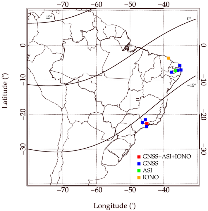
Figure 1Map indicating the geographic locations of the instruments used in this study. The red symbol represents the site where GNSS receiver, All-Sky Imager (ASI), and ionosonde (IONO) are available. Blue symbols represent sites with only GNSS receivers, while green symbols indicate ASI sites, and orange symbols represent IONO sites. The black lines identify the magnetic equator (0∘) and low latitudes (near ± 15∘) for the year 2016.
Table 2 shows more specific information about all the 10 sites where the instruments used in this study are located. Therefore, we used data from eight GNSS receivers (Campina Grande, João Pessoa, Afogados da Ingazeira, Natal, Cachoeira Paulista, Ubatuba, Inconfidentes, Varginha, São João do Cariri, and Fortaleza), two All-Sky Imagers (Cachoeira Paulista and São João do Cariri), and two ionosondes (Digisonde DPS4D model; Cachoeira Paulista and Fortaleza). We emphasize that these ionosondes operate with a min sampling interval in which the sounding frequencies range from 1.0 to 30.0 MHz (frequency step of 0.5 MHz; Reinish et al., 2009).
Table 2Latitude, longitude, and type of instrument present at the sites used in this study.
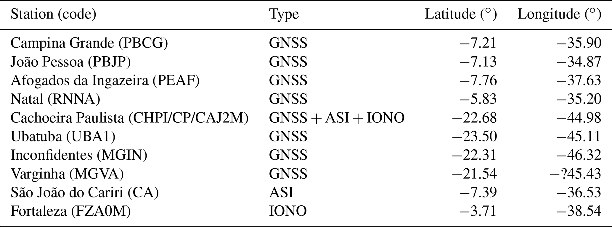
Specifically, we divided the data sites into two regions, namely equatorial and low latitudes. Thus, we obtained data from four dual-frequency GNSS receivers (PBCG, PBJP, PEAF, and RNNA), one All-Sky Imager (CA), and one ionosonde (FZA0M) for the equatorial region. The same was done for the low-latitudes region, where we collected data from four dual-frequency GNSS receivers (CHPI, MGIN, MGVA, and UBA1), one All-Sky Imager (CP), and one ionosonde (CAJ2M).
GNSS data were used for obtaining the TEC values for the DIX calculation during selected plasma bubble events from 2013 to 2020, which corresponds to the peak of solar cycle 24 up to the ascending phase of the solar cycle 25. In this regard, we used the methodology presented in Seemala and Valladares (2011) to obtain the TEC.
Moreover, we used the ASI data to identify the occurrence of plasma bubbles over the two regions. This analysis was performed by observing plasma depletions on the OI 630 nm emissions images, which were also used to estimate the times of the beginning and ending of the EPBs to support the analysis of the DIX responses observed during these events.
Furthermore, we also compared the DIX and ASI data to the ionograms from the equatorial and low-latitude ionosondes, which were used to identify the presence of spread F during the EPB events. These ionograms were generated from the Standard Archiving Output (SAO) files obtained from the ionosondes. Thus, these comparisons were discussed in terms of the spread F duration and intensity during the EPB responses observed using DIX.
In addition, we compared the DIX responses to EPBs with the solar activity level, as measured by the sunspot number during the period from 2013 to 2020, to evaluate the relation between the intensity of ionospheric disturbances with the season/solar activity. We emphasize that we selected EPB events that occurred near the summer of each year, aiming for a better comparison among them. In this regard, we also based our selection on data availability, considering the simultaneity of GNSS, ionosonde, and All-Sky Imager observations. Finally, we used only data from periods with no significant magnetic activity (Kp≤3) to avoid the effects of magnetic disturbances on DIX.
3.1 Validation of the DIX response to plasma bubbles
Figure 2 shows the time variations in the relative slant TEC (STEC; Fig. 2a), DIX (Fig. 2b), and ROTI (Fig. 2c) obtained on 30 January 2014, from the satellite PRN (pseudorandom noise) 3 observations of the following equatorial GNSS stations (left to right panels, respectively): PBCG, PBJP, PEAF, and RNNA. This figure also shows a sequence of OI 630 nm airglow images taken at CA (Fig. 2d, e, f, and g) during the same satellite PRN tracking time. Red arrows on these images indicate depletions associated with equatorial plasma bubbles.
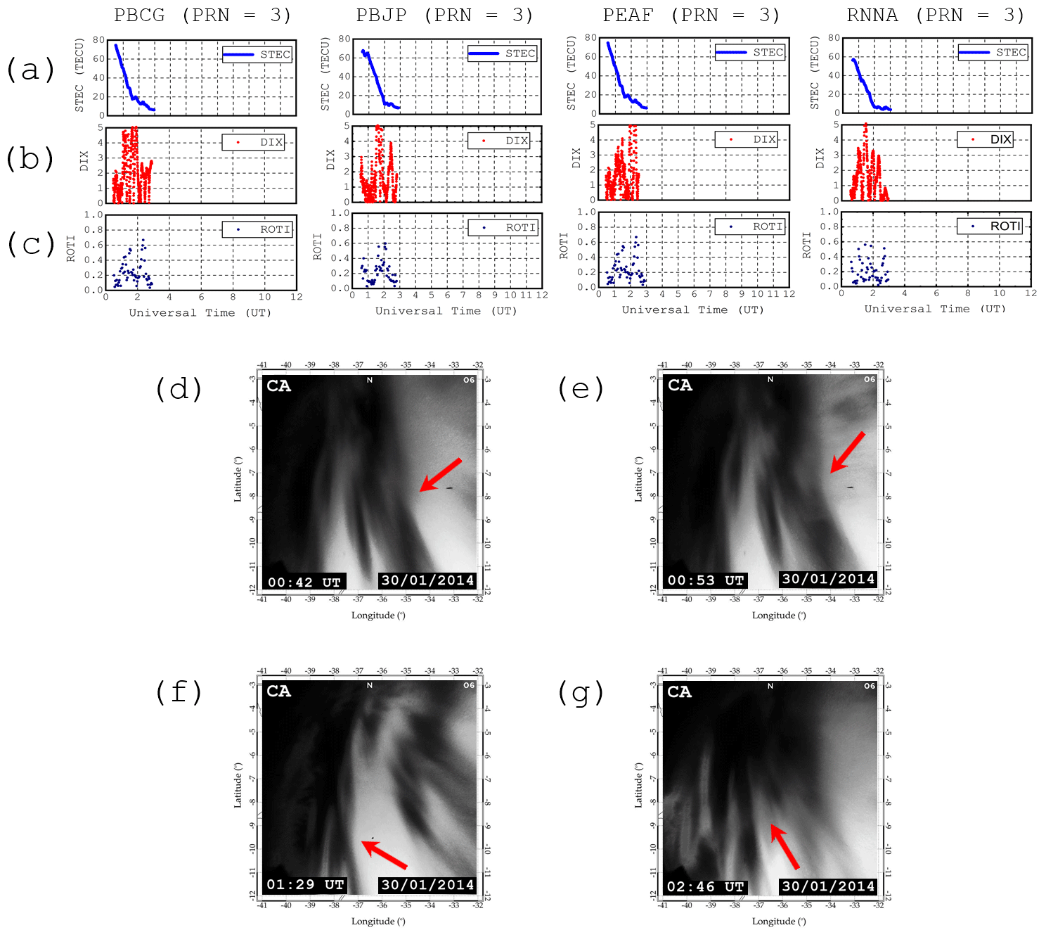
Figure 2Relative STEC (a), DIX (b), and ROTI (c) for PBCG, PBJP, PEAF, and RNNA observations, along with a sequence of OI 630 nm airglow images taken at CA (d, e, f, g) during the same satellite PRN 3 tracking time.
We observe a DIX enhancement associated with the TEC fluctuations due to the plasma bubble occurrence. Specifically, the depletions from 01:00 to 03:00 UT that are poorly visible, when considering only the STEC curve (Fig. 2a), appear as clear peaks in both DIX (Fig. 2b) and ROTI (Fig. 2c) during the same time interval in which both indices presented the highest values (DIX ∼ 5 and ROTI ∼ 0.6). This behavior is observed similarly but not identically over the four equatorial GNSS stations, which reinforces the idea that the DIX provides a localized response to the TEC variations associated with the occurrence of ionospheric disturbances (as suggested by Picanço et al., 2021). Moreover, since the ROTI is one of the most reliable indices for detecting TEC changes due to ionospheric irregularities, the simultaneous response of both indices is a good indication that the DIX is also capable of perceiving the presence of TEC fluctuations generated by plasma bubble events (Carmo et al., 2021). However, to ascertain the most likely origin of these disturbances, we analyzed OI 630 nm airglow images taken at CA (Fig. 2d–g), a site located at the center of the perimeter that is formed by the four equatorial GNSS stations. These ASI images show the typical plasma bubble signature, which is a field-aligned depletion with eastward motion (highlighted by the red arrows; Sobral et al., 1985).
Figure 3 shows the time variations in the relative STEC (Fig. 3a), DIX (Fig. 3b), and ROTI (Fig. 3c) obtained for 30 January 2014 from the satellite PRN 23 observations of the following low-latitude GNSS stations (left to right panels, respectively): CHPI, MGIN, MGVA, and UBA1. Also in this figure, a set of OI 630 nm airglow images taken at CP (Fig. 3d, e, f, and g) during the same satellite PRN tracking time is presented. The red arrows on these images indicate the depletions associated with equatorial plasma bubbles.
Then, we can observe that the first DIX peak is coherent with the time of occurrence of the first ROTI peak. In addition, we would like to emphasize that the DIX is not an index specifically to detect small-scale irregularities, such as the ROTI. The DIX is an index that responds to general TEC variations caused by internal (e.g., EPBs) and/or external (e.g., magnetic storms) sources.

Figure 3Relative STEC (a), DIX (b), and ROTI (c) for CHPI, MGIN, MGVA, and UBA1 observations, along with a sequence of OI 630 nm airglow images taken at CP (d, e, f, g) during the same satellite PRN 23 tracking time.
From this figure, it is reasonable to state that there is a clear DIX response to the plasma bubble occurrence, which is a result of the TEC depletions associated with this phenomenon. In this regard, we observe some small-scale fluctuations within the STEC (Fig. 3a) daily curve. However, independently analyzing these STEC variations appears not to be sufficient to evaluate the intensity of the TEC changes due to the plasma bubble event. Thus, by observing the projection of these disturbances in DIX (Fig. 3b) and ROTI (Fig. 3c), we noticed that both indices presented the highest values (DIX > 5 and ROTI ∼ 1) in the period for 03:30 through 05:30 UT. Since DIX and ROTI are raised to upper levels, it characterizes a considerably plasma bubble case.
In the next few hours (05:30 to 09:00 UT), both indices start to follow a gradual decrease from 03:30 through 06:00 UT, reaching the zero level. Just like in the analysis of the equatorial stations, this behavior agrees with the expected characteristic of plasma bubbles, which are a typical phenomenon of the nighttime ionosphere (Pimenta et al., 2001). In addition, the same gradual behavior was observed in all four low-latitude GNSS stations, which presented DIX and ROTI enhancements at almost the same time. To verify the most likely origin of these disturbances, we observed OI 630 nm airglow images taken at CP (Fig. 3d–g), a site located at the center of the perimeter formed by the four GNSS stations. These ASI images also showed the typical plasma bubble signature (highlighted by the red arrows). In addition, we provide more results from these cases in the Supplement accompanying this paper (Figs. S1 and S2). These figures show the DIX and ROTI (upper panels) time variations accompanied by the related STEC and VTEC (vertical total electron content; lower panels) curves. Furthermore, these results confirm that the EPB-related DIX and ROTI peaks occur at around the same time. We also observed non-EPB peaks on DIX, possibly associated with TEC variations that may not be necessarily related to plasma bubbles. Additional research is necessary to explain the origin of these peaks. However, this need is not within the scope of this work.
From those results, the DIX is able to detect the ionosphere response to plasma bubbles in terms of the intensity of changes in its electronic density. In this context, case studies focused on evaluating the ionospheric disturbances observed using DIX during plasma bubble events are presented in the next section.
3.2 Analysis of EPB-related ionospheric disturbances under high solar activity
In the present case study, we analyze the DIX responses during four selected plasma bubble events distributed along the period from around the peak (2013) to the midpoint of the descending phase (2016) of solar cycle 24.
Figure 4 shows the time variations in the DIX (left panels) for the equatorial (PBCG, PBJP, PEAF, and RNNA) and low-latitude (CHPI, MGIN, MGVA, and UBA1) GNSS stations during the following periods: 21–22 December 2013 (Fig. 4a), 1–2 February 2014 (Fig. 4b), 8–9 January 2015 (Fig. 4c), and 31 January–1 February 2016 (Fig. 4d). Along with the DIX graphs, this figure also includes OI 630 nm airglow images (middle panels) indicating the occurrence of plasma bubbles over both CA and CP ASI sites. We also present ionograms (right panels) from the FZA0M and CAJ2M ionosondes obtained at the same time periods of DIX calculation. To help visualize the EPB events behavior in more detail, we provide an extended collection of IONO and ASI images related to this case study in the Supplement accompanying this paper (Figs. S3 to S10). Blue bars on the DIX graphs indicate the time interval where bubble signatures were seen on the available ASI data. Yellow bars indicate the interval where spread F was observed in the ionograms. Red arrows on the OI 630 nm airglow images indicate depletions associated with equatorial plasma bubbles, while black arrows on the ionograms indicate the spread F occurrence. It is worth mentioning that ASI images can be affected by other atmospheric phenomena (e.g., clouds and rain), and the spread F observed in the ionograms tends to be more intense at the peak of the bubble passage over the ionosonde field of view. Therefore, we considered those factors to select snapshots that could facilitate the visibility of the plasma bubble signatures in data from both instruments.
In the first case (Fig. 4a), plasma bubble signatures were observed on the ASI and/or IONO data at São João do Cariri from 22:30 to 05:30 UT on 21–22 December 2013. It is emphasized that the same data were not available for Cachoeira Paulista for this period. Nonetheless, at around 23:00 UT, the DIX over both latitude ranges started to increase in response to the TEC depletions. We notice that the DIX over all stations responds to the EPB occurrence in the form of a gradual increase followed by a decrease as the bubble/spread F becomes weak. The DIX over the equatorial stations shows two peaks, with the first one around 01:30 UT and the second around 03:20 UT. This behavior can be attributed to the waveform zonal propagation of these bubbles, which produces cyclic longitudinal TEC variations (as reported in Takahashi et al., 2021). Following the same behavior, the DIX over low-latitude GNSS stations shows fluctuations simultaneously, reaching the first peak at 02:10 UT and the second one at ∼ 04:10 UT, which is 40 min later than in the equatorial stations. Therefore, we can state that DIX was able to estimate the latitudinal time of propagation of the EPB-related plasma disturbances between the equatorial and low-latitude regions. Those disturbances remain within the weakly disturbed state (DIX under 2) in both latitude ranges and last for about 5 h after their peaks. Notably, the low-latitude GNSS stations presented averagely higher DIX values than the equatorial ones during the plasma bubble occurrence. Such an effect can be explained by the presence of the equatorial ionization anomaly (EIA) southern crest, which produces a large amount of plasma in this region, also making the TEC percentage changes higher (Abdu, 1997). Specifically, the EIA is characterized mainly by a plasma trough centered in the equatorial region, flanked by two crests over low latitudes, generally occurring at around ± 15∘ dip latitude (Rastogi et al., 1990). Moreover, the EIA crests present a high day-to-day variability, which can suddenly change their position (Takahashi et al., 2016). Since we are using data from four nearby GNSS stations at low latitudes, the EIA southern crest might be above or below those stations over time. Consequently, DIX values at low-latitude stations might eventually be higher than those over the magnetic equator, considering that those stations are under the influence of the southern EIA crest and can be directly affected by its dynamics.
The second case (Fig. 4b) shows the occurrence of plasma bubbles on 1–2 February 2014. This event was registered as spread F on the FZA0M ionograms from 22:00 to 05:30 UT. Ionosonde data from Cachoeira Paulista was not available during this period. However, plasma bubble signatures were seen on the available ASI data over this station from 23:30 to 05:30 UT. Nevertheless, in response to this plasma bubble event, the DIX over equatorial GNSS stations started to rise at around 22:10 UT, followed by a peak at 01:20 UT (DIX under 3; disturbed state). Afterward, these disturbances lasted for about 4 h after the peak. On the low-latitude stations, the DIX increases took place at almost the same time (first over the MGIN station). In contrast, the DIX peak occurred more than 1 h later (∼ 02:20 UT), and these disturbances lasted for about 5 h after this peak (DIX under 3; disturbed state). Therefore, these disturbances started at almost the same time and followed the same gradual behavior as in the equatorial stations but lasted longer. Since the DIX is an ionospheric index that responds to several types of ionospheric phenomena, we highlight that the disturbances observed over the equatorial stations were caused not only by the plasma bubble event. These effects can be attributed to the slower ionospheric recombination occurring in the EIA region, which was confirmed by the TEC curve behavior (not shown here). Thus, it is possible that the ionosphere over low latitudes remained disturbed 1 h after the end of the plasma bubble event. However, since this analysis is beyond the scope of the present study, we intend to explain this in more detail in a further paper.
The third case (Fig. 4c) shows plasma bubbles registered on the ASI and/or IONO data at São João do Cariri from 22:00 to 07:20 UT on 8–9 January 2015. Moreover, ionograms from the FZA0M ionosonde showed spread F signatures from 00:00 to 01:30 UT and from 02:20 to 04:40 UT on 9 January 2015. It was not possible to see the bubble signatures on the OI 630 nm airglow images obtained over CP since there was not enough sky visibility for this period. The DIX over all the stations started to rise before 21:00 UT. Nonetheless, these DIX increases precede the beginning phase of the plasma bubble event, which is related to local disturbances over both equatorial and low-latitude regions. These disturbances can be caused by changes in the E-region dynamo that occur during geomagnetic quiet periods and cause the recombination of electrons and ions to be anticipated in comparison to the reference day used in the DIX calculation (Rishbeth, 1991; Fuller-Rowell et al., 1996; Kelley, 2009). Besides that, a peak at ∼ 22:30 UT is observed on the DIX curve over all the equatorial stations, which occurs immediately after the EPB time of rising. In the low-latitude ionospheric region, the DIX peaks occur at 00:10 UT, within an interval of 1:40 h after the peaks observed in the equatorial region. In these hours, we observed the spread F in the ionograms from the CAJ2M ionosonde. After that, small DIX fluctuations are observed in both latitude ranges. However, these fluctuations tend to stop with the end of the plasma bubble event (after ∼ 07:20 UT).
Last, the fourth case (Fig. 4d) presents a plasma bubble event registered on the ASI and/or IONO data from 21:50 to 07:40 UT at São João do Cariri and from 23:30 to 04:20 UT at Cachoeira Paulista between 31 January and 1 February 2015. The OI 630 nm airglow images from the CA ASI started to present bubble signatures at 21:50 UT on 31 January. After that, at 22:00 UT, the DIX over equatorial GNSS stations presented an enhancement, which evolved to a first peak at 23:59 UT. The same behavior is seen over low-latitude stations but with these initial peaks happening 30 min later, at 00:29 UT. Then, two more peaks are seen on the DIX over the equatorial region; the first one is at 01:50 UT, and the second is at ∼ 04:30 UT. These peaks also occur in the low-latitudes DIX, at 02:40 and 04:50 UT, respectively. Additionally, these times represent a 50 and 20 min delay concerning the equatorial region, which indicates that the average latitudinal EPB propagation time between the latitude ranges was about 33 min.
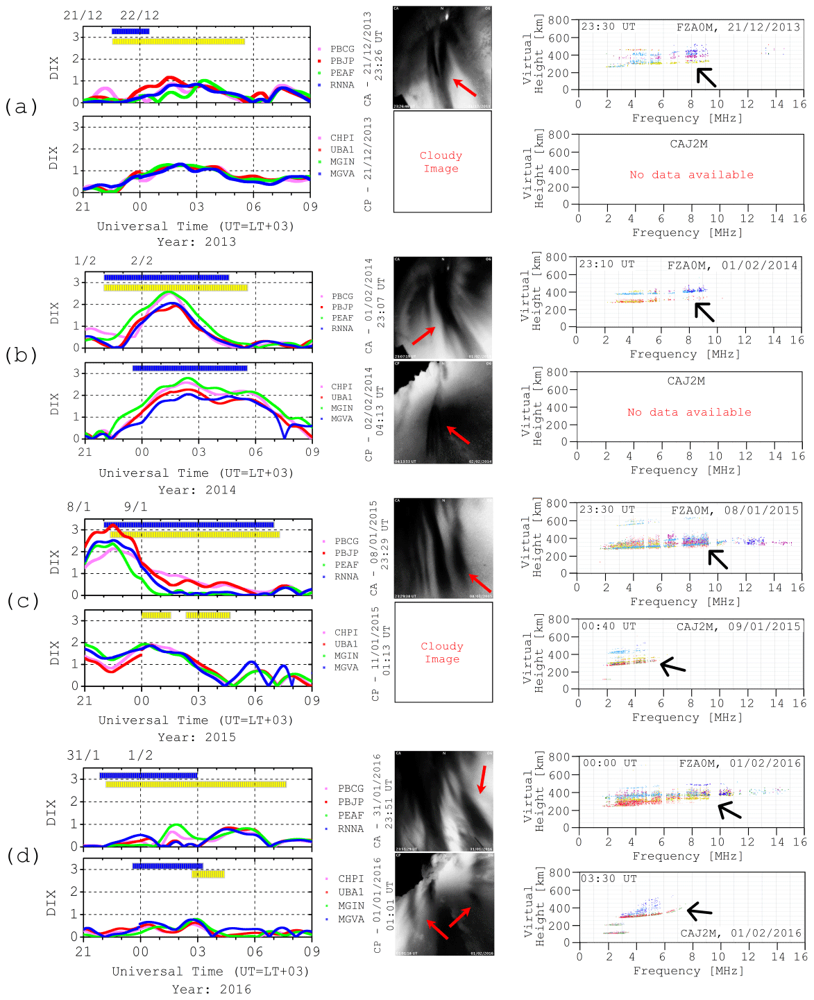
Figure 4Time variations in the DIX (left panels) for equatorial and low-latitude stations, along with OI 630 nm airglow images (middle panels) taken at CA and CP, and ionograms (right panels) showing the spread F occurrence at FZA0M and CAJ2M on 21–22 December 2013 (a), 1–2 February 2014 (b), 8–9 January 2015 (c), and 31 January–1 February 2016 (d).
We notice that, in some EPB events, the DIX responses were not observed simultaneously at equatorial and low-latitude GNSS stations. We attribute this to the dynamic of the plasma depletion in different latitude ranges. In this regard, Dabas et al. (1992) calculate the EPB latitudinal velocity from the time difference in the depletions observed between an equatorial and a low-latitude station. Bringing this concept to the context presented here, we take the case shown in Fig. 4d as an example. We observed 20 to 50 min time delays between the EPB peaks in DIX over both latitude ranges. In addition, the bubble signature did not fully reach the CP ASI field of view. Therefore, we suggest that this bubble event developed slower than the others, where the time delays were not significant. Consequently, DIX values at low-latitude stations remained lower since only partial plasma bubble signatures reached this region, and this event developed slower.
3.3 Analysis of EPB-related ionospheric disturbances under low solar activity
In this case study, we analyze the DIX response to plasma bubbles during four selected events distributed throughout the period that starts around the cycle 24 descending phase (2017) up to the ascending phase (2020) of solar cycle 25.
Figure 5 shows the time variations in the DIX (left panels) for the equatorial (PBCG, PBJP, PEAF, and RNNA) and low-latitude (CHPI, MGIN, MGVA, and UBA1) GNSS stations during the following periods: 23–24 February 2017 (Fig. 5a), 5–6 January 2018 (Fig. 5b), 20–21 December 2019 (Fig. 5c), and 20–21 March 2020 (Fig. 5d). Additionally, this figure also shows OI 630 nm airglow images (mid panels) taken at the CA and CP ASI sites, which indicate the occurrence of plasma bubbles around the same time periods of the DIX calculation. Along with these figures, we present examples of ionograms (right panels) from the FZA0M and CAJ2M ionosondes in which we see the spread F occurrence. To help visualize the EPB event behavior in more detail, we provide an extended collection of IONO and ASI images related to this case study in the Supplement accompanying this paper (Figs. S11 to S18). Blue bars on the DIX graphs indicate the time interval where bubble signatures were seen on the available ASI data. Yellow bars indicate the interval where spread F was observed in the ionograms. Red arrows on the OI 630 nm airglow images indicate depletions associated with equatorial plasma bubbles, while black arrows on the ionograms indicate the spread F occurrence.
In the first case (Fig. 5a), plasma bubble signatures were observed on the ASI and/or IONO data from 22:00 to 07:20 UT at São João do Cariri on 23–24 February 2017 and from 00:30 to 04:50 UT at Cachoeira Paulista on 24 February 2017. In response to these events, the DIX over the equatorial GNSS stations starts to rise at ∼ 22:20 UT, following a gradual increasing behavior until it reaches to a peak at around 01:20 UT. However, we notice that this peak occurs approximately 1 h earlier at the PEAF GNSS station, which is ∼ 200 km west of PBCG. Since the EPBs move eastward in this case, we can state that DIX also responds to the zonal propagations of these phenomena. Furthermore, the bubble event did not reach all the low-latitude stations. In such case, we observe only small fluctuations within the DIX first scale on these locations. Then, we observe a peak in the DIX over these stations at 03:00 UT, within an interval of 1:40 h after the peaks observed in the equatorial region. This behavior matches with the third case presented in the previous section, where the latitudinal propagation of the bubble event was of the same order of time. Therefore, we can state that the DIX also responds to the latitudinal development of plasma bubbles since the observed disturbances presented a similar temporal pattern. Finally, we see that as the bubble event comes to an end, the DIX starts decreasing in both latitude ranges, returning to the initial non-perturbed state.
The second case (Fig. 5b) shows the occurrence of plasma bubbles that were registered on the ASI and/or IONO data at São João do Cariri from 22:00 to 05:30 UT on 5–6 January 2018. Moreover, ionograms from the CAJ2M ionosonde showed spread F signatures from 02:00 to 04:30 UT on 6 January 2018. It was not possible to see the bubble signatures on the OI 630 nm airglow images obtained over CP since there was not enough sky visibility. Furthermore, the DIX over the equatorial GNSS stations already presented an increasing behavior before 21:00 UT, which is probably associated with disturbances driven by the neutral atmosphere (as reported in Picanço et al., 2021). These ionospheric disturbances peak at around 22:30 UT, and the DIX later starts to decline. Then, with the plasma bubble growth, the DIX over this region increases again, reaching the first peak at around 23:30 UT. At low latitudes, the DIX curves continue to show a decreasing behavior associated with perturbations prior to the plasma bubble event. It is interesting to note that this decreasing behavior ceases at around 02:20 UT, immediately after spread F signatures are seen in the ionograms of the CAJ2M ionosonde. We notice that the DIX over the equatorial region presented a peak at around the same time, surpassing the weakly disturbed scale (DIX under 2; Denardini et al., 2020a). At first, we can state that the plasma bubble event was intense enough to disturb the low-latitude ionosphere for a short period since the spread F signatures were only observed during the time of occurrence of this peak. Finally, the DIX over both latitude ranges started to decrease after the end of the plasma bubble event, remaining close to zero.
Figure 5c shows plasma bubbles registered on the ASI and/or IONO data at São João do Cariri from 22:00 to 07:00 UT on 20–21 December 2019. Additionally, ionograms from the CAJ2M ionosonde show spread F signatures during the period from 03:40 to 06:50 UT on 21 December 2019. Since the available OI 630 nm airglow images over CP were cloudy for almost the entire period of study, it was not possible to observe the presence/absence of bubble signatures on it. Moreover, the DIX over the equatorial GNSS stations shows a peak at around 22:30 UT, after the beginning of the plasma bubble growth phase. After that, small DIX fluctuations occur until the end of the plasma bubble event. In the region of low latitudes, the DIX does not show higher values during the initial period of the bubble development. The absence of spread F in the ionograms obtained between 21:00 and 03:50 UT at CAJ2M indicates that the bubble did not change the TEC at low latitudes to generate strong disturbances. However, as the irregularities start to develop spread F in the CAJ2M ionograms (03:50 to 06:50 UT), we can see a gradual increase in DIX, which reaches a peak at 06:50 UT. This feature reinforces that the DIX is strongly related to the physical variations in the ionosphere that are measured by the ionosonde (Denardini et al., 2020b).
Finally, Fig. 5d presents a plasma bubble event registered on the ASI and/or IONO data from 22:30 to 04:40 UT at São João do Cariri on 20–21 March 2020. In addition, it was not possible to observe bubble signatures on the OI 630 nm airglow images obtained over CP since there was not enough sky visibility for that. Furthermore, the ionograms from the CAJ2M ionosonde did not show spread F signatures during the entire period of study. Nevertheless, the DIX over the equatorial latitudes started to rise at around 22:45 UT, which is 15 min after the bubble event start is observed on the ASI images. On the other hand, the DIX over low latitudes did not show any abrupt variations when the equatorial ionosphere showed DIX disturbances. In the absence of spread F on the ionograms from the CAJ2M ionosonde, it is reasonable to state that this EPBs event was not strong enough to generate TEC depletions detectable by DIX. It is noteworthy that the DIX over the equatorial GNSS stations presented a pulse-like response in the presence of plasma bubbles/spread F, while the ionosphere over low latitudes behaved similarly to the expected for non-disturbed periods, without the concurrent DIX response since no spread F was registered.
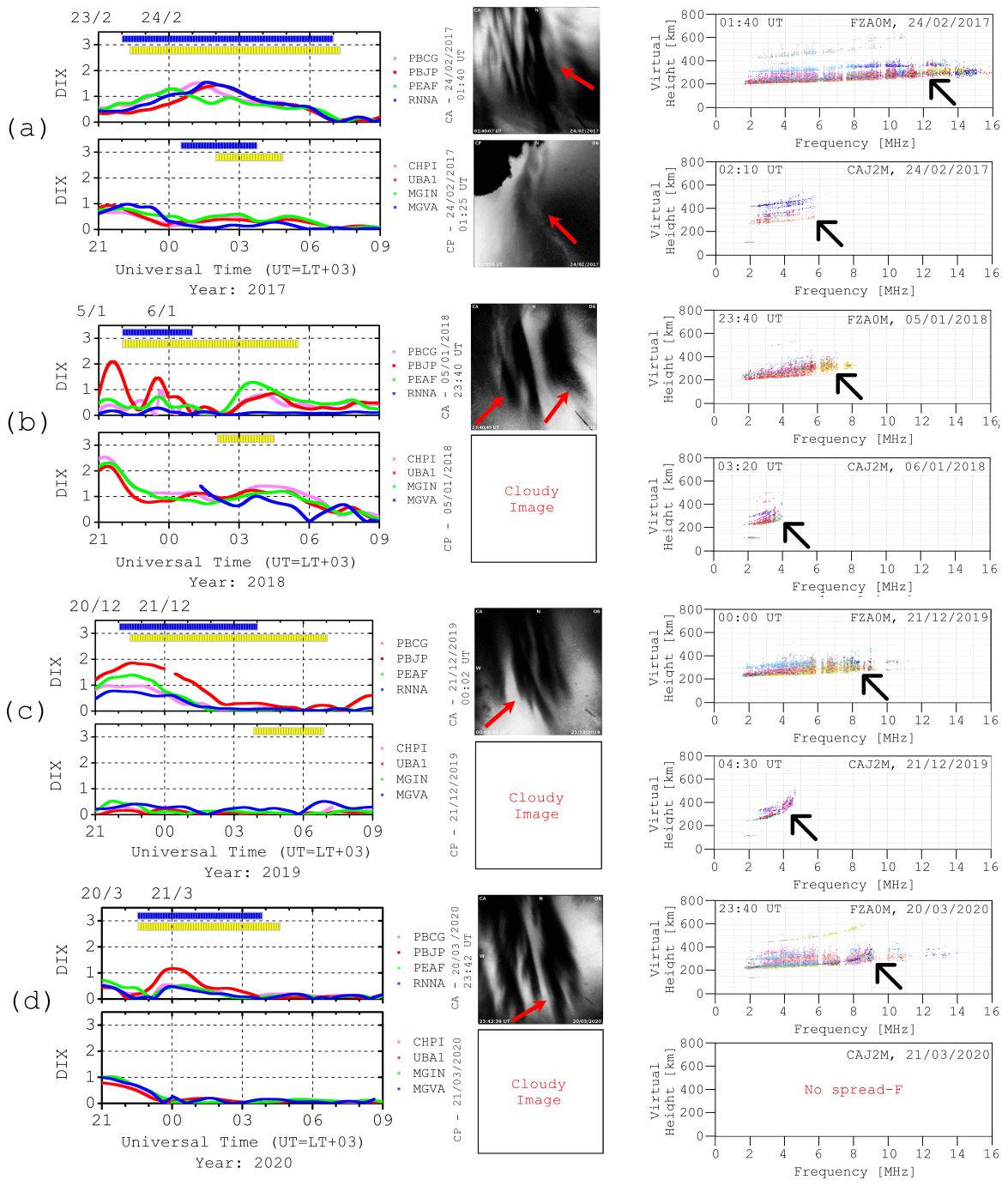
Figure 5Time variations in the DIX for equatorial and low-latitude stations, along with OI 630 nm airglow images taken at CA and CP, and ionograms showing the spread F occurrence at FZA0M and CAJ2M on 23–24 February 2017 (a), 5–6 January 2018 (b), 20–21 December 2019 (c), and 20–21 March 2020 (d).
3.4 Overview of the ionospheric disturbances observed during solar cycle 24–25
We analyzed the DIX values calculated during each of the studied plasma bubble events from 2013 to 2020, as presented in Sect. 3.2 and 3.3. In addition, we have also selected more periods for this analysis, intending to perform more reliable statistics, corresponding to five events per year. Specifically, we first obtained the maximum DIX values during the bubbles' passage over each station for each event. Then, we calculated an average of these max values for each event/year, considering the four equatorial (PBCG, PBJP, PEAF, and RNNA) and low-latitude (CHPI, UBA1, MGIN, and MGVA) GNSS stations. This analysis was performed to compare the amplitude of DIX peaks caused by plasma bubbles with the solar cycle 24–25 variation. We reinforce that we selected only geomagnetic quiet days (Kp≤3) to avoid the effects of magnetic disturbances on DIX. Thus, Table 3 presents a summary of the averaged maximum DIX values observed during the EPB cases selected from 2013 to 2020.
Table 3Summary of the averaged maximum DIX values attributed to plasma bubble events selected from 2013 to 2020 for the following GNSS stations analyzed: PBCG, PBJP, PEAF, RNNA, CHPI, UBA1, MGIN, and MGVA.
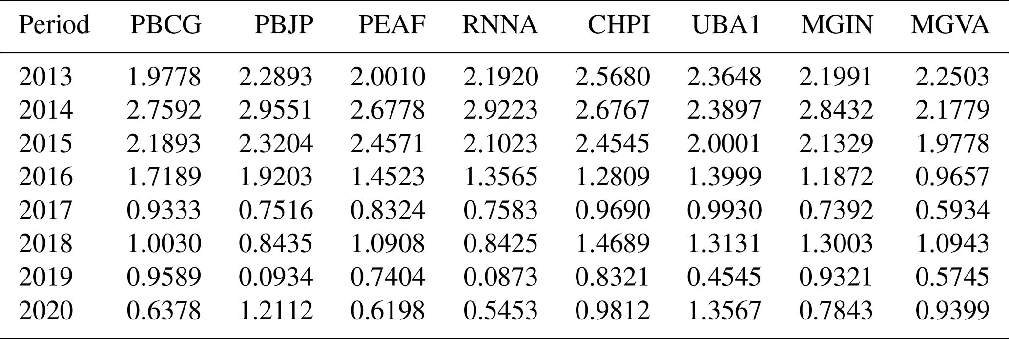
Figure 6 shows the time variation in the averaged maximum DIX values during the studied plasma bubble events shown in Table 3 for the equatorial (Fig. 6a) and low latitudes (Fig. 6b), along with the yearly mean total sunspot number curve (navy line).
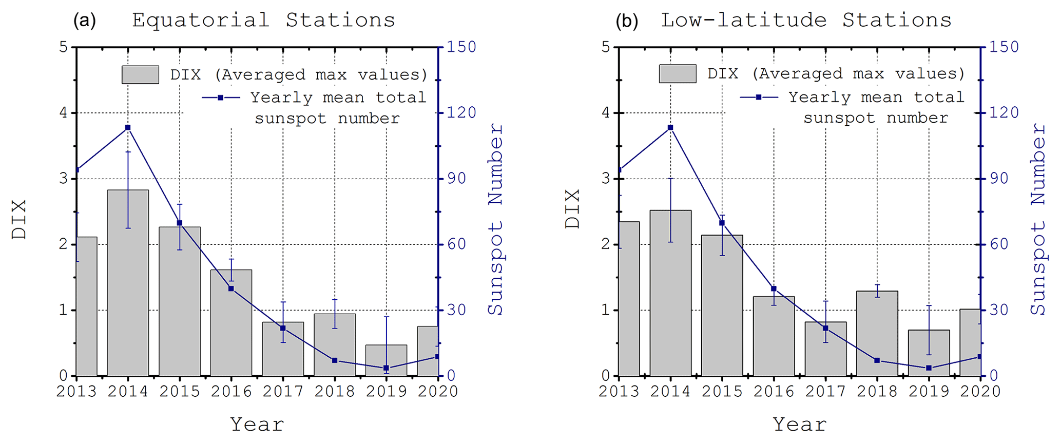
Figure 6Averaged max DIX time variation during selected EPBs events observed from 2013 to 2020 over the equatorial (a) and low-latitude (b) GNSS stations along with the yearly mean total sunspot number for the same period.
From the results presented in Fig. 6 and Table 3, we have noticed that the EPB-related disturbances in DIX tend to follow the trend of solar activity, which is represented by the variation in the yearly mean total sunspot number. In this context, the highest disturbances due to EPBs occurred between 2014 and 2015 over both equatorial and low-latitude GNSS stations. This period coincides with the peak of solar activity in cycle 24 (around 2014), where the mean sunspot number was approximately 113. Specifically, in the equatorial region, we observed that the intensity of the EPB-related DIX responses closely followed the variations in the solar activity level between 2014 and 2017. However, we can observe small fluctuations within the DIX scale in the years 2013 and 2018. In this context, it is noteworthy to mention that the DIX is an index for ionospheric disturbances in general that responds not only to EPBs. Therefore, as presented by Picanço et al. (2021), it is reasonable to state that the DIX for 2013 and 2018 may also embed small non-EPB TEC disturbances. Besides that, the disturbances present an increase from 2013 to 2014, which is followed by a decreasing average behavior until the beginning of solar cycle 25 in 2020. On the other hand, the low-latitude region showed a trend of variation much more consistent with the solar activity level, except for the plasma bubble events observed in 2018. In this event, the DIX values remained above the scale of nearby events.
Despite the observation of events with slightly variable magnitudes, TEC disturbances observed during the solar cycle 24–25 followed the trend of solar activity during most of the period studied. Therefore, the EPB-related ionospheric disturbances observed using the DIX are expected to behave according to seasonal and solar activity characteristics. However, it is important to mention that the ionosphere degree of perturbation during these events can also be influenced by non-EPB phenomena that may occur simultaneously with the presence of plasma bubbles.
In short, these results indicate a clear solar activity dependence of the plasma bubbles' intensity on the solar cycle. Since few studies on the solar activity variation in the plasma bubbles' physical characteristics are found in the literature, these results are important for understanding how EPBs disturb the ionosphere along the solar cycle stages. For instance, Agyei-Yeboah et al. (2019) presented a study of the EPBs occurrence rate during the solar cycle 23–24 over the Brazilian equatorial region. The authors stated that plasma bubbles tend to be more frequent during high solar activity, followed by moderate and low solar activity conditions. In this context, the results presented here indicate that EPBs are also more intense around the peak of solar cycles for both equatorial and low-latitude Brazilian regions.
This paper analyzed the ionospheric total electron content responses to plasma bubbles by using ionosonde, all-sky imager, and GNSS data over Brazilian equatorial and low-latitude stations. The results were discussed in terms of the disturbance ionosphere index behavior under different solar activity levels and compared to other well-established parameters found in the literature. We summarize the conclusions below as follows:
-
The DIX proved able to detect the TEC perturbations generated by weak, moderate, and strong plasma bubble events. In those EPB cases, the DIX presented a gradual increase as the bubbles started to grow and tended to return to their initial non-perturbed behavior at the end of the plasma bubble events.
-
The DIX over all studied GNSS stations also responded to the presence of spread F on the ionograms obtained from equatorial and low-latitude ionosondes. In this context, the DIX behavior matched the intensity of spread F, which was higher or slower according to the ionograms' characteristics. Additionally, the occurrence of spread F in all ionograms coincided with peaks observed in DIX over both equatorial and low-latitude GNSS stations.
-
We observed a delay in the DIX response time to EPBs between low-latitude and equatorial GNSS stations in some of the studied cases (2013, 2014, and 2016). For instance, this time delay was 40 min during the first case (2013). Therefore, we suggest that it is the latitudinal propagation time of the EPB-related plasma disturbances between equatorial and low-latitude regions, which is a new feature observed using DIX. Therefore, the DIX can estimate the propagation time of the EPB-related ionospheric disturbances between latitude ranges.
-
The DIX also responded to the EPB eastward longitudinal propagations in some cases, where the first disturbances occurred 1 h earlier at the western equatorial GNSS station (PEAF), which is ∼ 200 km away from the center (PBCG) of the equatorial study area. Thus, the DIX can also estimate the propagation time of the EPB-related ionospheric disturbances between longitude ranges.
-
The contribution of neutral atmospheric effects may have intensified some DIX disturbances observed during the EPB periods. Since the DIX is an index that responds to several phenomena, we emphasize that the ionospheric TEC can remain disturbed even after the end of the plasma bubble event due to other phenomena.
-
Despite observing events with slightly variable magnitudes, TEC disturbances observed during the solar cycle 24–25 followed the trend of solar activity during most of the period studied. Therefore, the EPB-related ionospheric TEC disturbances are expected to behave according to seasonal and solar activity characteristics. However, it is important to mention that the ionosphere degree of perturbation during these events can also be influenced by non-EPB phenomena that may occur simultaneously with the presence of plasma bubbles.
The model (GPS-TEC software) for obtaining total electron content values is available at https://seemala.blogspot.com (Seemala, 2020).
The data used in the present study are fully open source and accessible on an acknowledgement basis from the Embrace/INPE Program website (http://www.inpe.br/spaceweather, Denardini et al., 2016). The sunspot data are available online from the NOAA website (https://www.ngdc.noaa.gov/stp/solar/ssndata.html, U.S. National Geophysical Data Center, 2013).
The supplement related to this article is available online at: https://doi.org/10.5194/angeo-40-503-2022-supplement.
GASP conceived the study, designed the data analysis, and lead the writing of the paper. CMD and PABN assisted in designing the study and the data analysis. LCAR assisted in designing the study and processing the ionospheric data analysis. CSC assisted in reviewing the paper and discussing the results of the study. SSC assisted in processing the interplanetary data analysis and discussing the results of the study. PFBN and ERH assisted in reviewing the paper and discussing the results of the study. All the authors helped to write and revise the paper.
The contact author has declared that none of the authors has any competing interests.
Publisher's note: Copernicus Publications remains neutral with regard to jurisdictional claims in published maps and institutional affiliations.
This article is part of the special issue “From the Sun to the Earth's magnetosphere–ionosphere–thermosphere”. It is a result of the VIII Brazilian Symposium on Space Geophysics and Aeronomy & VIII Symposium on Physics and Astronomy, Brazil, March 2021.
We would like to thank the Embrace/INPE Space Weather Program, for providing the ionosonde and All-Sky Imager data, the Brazilian Institute of Geography and Statistics (IBGE), for providing the raw GNSS data, and the CNPq/MCTIC and the Capes/MEC financial programs, for supporting the authors of this research.
This research has been supported by the Coordination for the Improvement of Higher Education Personnel (Capes/MEC; grant nos. 88887.467444/2019-00, 88887.685060/2022-00, 88887.1622967/2016, and 88887.362982/2019-00), the National Council for Scientific and Technological Development (CNPq/MCTI; grant nos. 303643/2017-0 and 150261/2022-5), and the National Space Science Center, Chinese Academy of Sciences (grant no. NSSC/CAS).
This paper was edited by Dalia Buresova and reviewed by two anonymous referees.
Aarons, J.: Global morphology of ionospheric scintillations, Proc. IEEE, 70, 360–378, https://doi.org/10.1109/PROC.1982.12314, 1982.
Aarons, J., Mendillo, M., Yantosca, R., and Kudeki, E.: GPS phase fluctuations in the equatorial region during the MISETA 1994 campaign, J. Geophys. Res.-Space, 101, 26851–26862, https://doi.org/10.1029/96ja00981, 1996.
Abdu, M. A.: Major phenomena of the equatorial ionosphere-thermosphere system under disturbed conditions, J. Atmos. Sol.-Terr. Phys., 59, 1505–1519, https://doi.org/10.1016/s1364-6826(96)00152-6, 1997.
Agyei-Yeboah, E., Paulino, I., Fragaso de Medeiros, A., Arlen Buriti, R., Roberta Paulino, A., Essien, P., Otoo Lomotey, S., Takahashi, H., and Max Wrasse, C.: Seasonal variation of plasma bubbles during solar cycle 23–24 over the Brazilian equatorial region, Adv. Space Res., 64, 1365–1374, https://doi.org/10.1016/j.asr.2019.06.041, 2019.
Astafyeva, E., Zakharenkova, I., and Förster, M.: Ionospheric response to the 2015 St. Patrick's Day storm: A global multi-instrumental overview, J. Geophys. Res.-Space, 120, 9023–9037, https://doi.org/10.1002/2015ja021629, 2015.
Borries, C., Wilken, V., Jacobsen, K. S., García-Rigo, A., Dziak-Jankowska, B., Kervalishvili, G., Jakowski, N., Tsagouri, I., Hernández-Pajares, M., Ferreira, A. A., and Hoque, M. M.: Assessment of the capabilities and applicability of ionospheric perturbation indices provided in Europe, Adv. Space Res., 66, 546–562, https://doi.org/10.1016/j.asr.2020.04.013, 2020.
Carmo, C. S., Denardini, C. M., Figueiredo, C. A. O. B., Resende, L. C. A., Picanço, G. A. S., Barbosa Neto, P. F., Nogueira, P. A. B., Moro, J., and Chen, S. S.: Evaluation of different methods for calculating the ROTI index over the Brazilian sector, Radio Sci., 56, e2020RS007140, https://doi.org/10.1029/2020RS007140, 2021.
Carrano, C. S., Groves, K. M., and Rino, C. L.: On the Relationship Between the Rate of Change of Total Electron Content Index (ROTI), Irregularity Strength (CkL), and the Scintillation Index (S4), J. Geophys. Res.-Space, 124, 2099–2112, https://doi.org/10.1029/2018JA026353, 2019.
Cherniak, I., Krankowski, A., and Zakharenkova, I.: ROTI Maps: a new IGS ionospheric product characterizing the ionospheric irregularities occurrence, GPS Solutions, 22, 1–12, https://doi.org/10.1007/s10291-018-0730-1, 2018.
Chu, F. D., Liu, J. Y., Takahashi, H., Sobral, J. H. A., Taylor, M. J., and Medeiros, A. F.: The climatology of ionospheric plasma bubbles and irregularities over Brazil, Ann. Geophys., 23, 379–384, https://doi.org/10.5194/angeo-23-379-2005, 2005.
Dabas, R. S., Banerjee, P. K., Bhattacharya, S., Reddy, B. M., and Singh, J.: Study of equatorial plasma bubble dynamics using GHz scintillation observations in the Indian sector, J. Atmos. Terr. Phys., 54, 893–901, https://doi.org/10.1016/0021-9169(92)90056-q, 1992.
Denardini, C. M., Dasso, S., and Gonzalez-Esparza, J. A.: Review on space weather in Latin America, 2. The research networks ready for space weather, Adv. Space Res., 58, 1940–1959, https://doi.org/10.1016/j.asr.2016.03.013, 2016 (data available at: http://www2.inpe.br/climaespacial/portal/en/, last access: 18 July 2022).
Denardini, C. M., Picanço, G. A. S., Barbosa Neto, P. F., Nogueira, P. A. B., Carmo, C. S., Resende, L. C. A., Moro, J., Chen, S. S., Romero-Hernandez, E., Silva, R. P., and Bilibio, A. V.: Ionospheric scale index map based on TEC data for space weather studies and applications, Space Weather, 18, 1–18, https://doi.org/10.1029/2019sw002328, 2020a.
Denardini, C. M., Picanço, G. A. S., Barbosa Neto, P. F., Nogueira, P. A. B., Carmo, C. S., Resende, L. C. A., Moro, J., Chen, S. S., Romero-Hernandez, E., Silva, R. P., and Bilibio, A. V.: Ionospheric scale index map based on TEC data during the Saint Patrick magnetic storm and EPBs, Space Weather, 18, 1–20, https://doi.org/10.1029/2019sw002330, 2020b.
Doherty, P., Raffi, E., Klobuchar, J. A., and EI-Arini, M. B.: Statistics of Time Rate of Change of Ionospheric Range Delay, Proceedings of ION GPS-94, Salt Lake City, 1589–1599, https://www.ion.org/publications/abstract.cfm?articleID=3981 (last access: 18 July 2022), 1994.
Figueiredo, C. A. O. B., Takahashi, H., Wrasse, C. M., Otsuka, Y., Shiokawa, K., and Barros, D.: Medium-Scale Traveling Ionospheric Disturbances Observed by Detrended Total Electron Content Maps Over Brazil, J. Geophys. Res.-Space, 123, 2215–2227, https://doi.org/10.1002/2017ja025021, 2018.
Fuller-Rowell, T. J., Codrescu, M. V., Rishbeth, H., Moffett, R. J., and Quegan, S.: On the seasonal response of the thermosphere and ionosphere to geomagnetic storms, J. Geophys. Res.-Space, 101, 2343–2353, https://doi.org/10.1029/95ja01614, 1996.
Gulyaeva, T. L. and Stanislawska, I.: Derivation of a planetary ionospheric storm index, Ann. Geophys., 26, 2645–2648, https://doi.org/10.5194/angeo-26-2645-2008, 2008.
Jakowski, N. and Hoque, M. M.: Estimation of spatial gradients and temporal variations of the total electron content using ground based GNSS measurements, Space Weather, 17, 339–356, https://doi.org/10.1029/2018sw002119, 2019.
Jakowski, N., Stankov, S. M., Schlueter, S., and Klaehn, D.: On developing a new ionospheric perturbation index for space weather operations, Adv. Space Res., 38, 2596–2600, https://doi.org/10.1016/j.asr.2005.07.043, 2006.
Jakowski, N., Borries, C., and Wilken, V.: Introducing a disturbance ionosphere index, Radio Sci., 47, RS0L14, https://doi.org/10.1029/2011RS004939, 2012.
Kersley, L., Malan, D., Pryse, S. E., Cander, L. R., Bamford, R. A., Belehaki, A., Leitinger, R., Radicella, S. M., Mitchell, C. N., and Spencer, P. S. J.: Total electron content: a key parameter in propagation: measurement and use in ionospheric imaging, Ann. Geophys., 47, 1067–1091, https://doi.org/10.4401/ag-3286, 2004.
Kelley, M. C.: The Earth's Ionosphere: plasma physics and electrodynamics, International Geophysics Series, Vol. 96, 2 Edn., Academic Press, Burlington, MA, ISBN 10 0120884259, 13 978-0120884254, 2009.
Kintner, P. M., Ledvina, B. M., and de Paula, E. R.: GPS and ionospheric cintillations, Space Weather, 5, 1–23, https://doi.org/10.1029/2006SW000260, 2007.
Liu, Y., Li, Z., Fu, L., Wang, J., Radicella, S. M., and Zhang, C.: Analyzing Ionosphere TEC and ROTI Responses on 2010 August High Speed Solar Winds, IEEE Access, 7, 29788–29804, https://doi.org/10.1109/ACCESS.2019.2897793, 2019a.
Liu, Z., Yang, Z., Xu, D., and Morton, Y. J.: On inconsistent ROTI derived from multiconstellation GNSS measurements of globally distributed GNSS receivers for ionospheric irregularities characterization, Radio Sci., 54, 215–232, https://doi.org/10.1029/2018RS006596, 2019b.
Nogueira, P. A. B., Abdu, M. A., Batista, I. S., and de Siqueira, P. M.: Equatorial ionization anomaly and thermospheric meridional winds during two major storms over Brazilian low latitudes, J. Atmos. Sol.-Terr. Phys., 73, 1535–1543, https://doi.org/10.1016/j.jastp.2011.02.008, 2011.
Otsuka, Y., Ogawa, T., Saito, A., Tsugawa, T., Fukao, S., and Miyazaki, S.: A new technique for mapping of total electron content using GPS network in Japan, Earth Planet. Space, 54, 63–70, https://doi.org/10.1186/BF03352422, 2002.
Pi, X., Mannucci, A. J., Lindqwister, U. J., and Ho, C. M.: Monitoring of global Ionospheric irregularities using the Worldwide GPS Network, Geophys. Res. Lett., 24, 2283–2286, https://doi.org/10.1029/97GL02273, 1997.
Picanço, G. A. S., Denardini, C. M., Nogueira, P. A. B., Barbosa-Neto, P. F., Resende, L. C. A., Carmo, C. S., Romero-Hernandez, E., Chen, S. S., Moro, J., and Silva, R. P.: Evaluation of the non-perturbed TEC reference of a new version of the DIX, Braz. J. Geophys., 38, 1–10, https://doi.org/10.22564/rbgf.v38i3.2056, 2020.
Picanço, G. A. S., Denardini, C. M., Nogueira, P. A. B., Barbosa-Neto, P. F., Resende, L. C. A., Chen, S. S., Carmo, C. S., Moro, J., Romero-Hernandez, E., and Silva, R. P.: Equatorial ionospheric response to storm-time electric fields during two intense geomagnetic storms over the Brazilian region using a Disturbance Ionosphere indeX, J. Atmos. Sol.-Terr. Phys., 223, 105734, https://doi.org/10.1016/j.jastp.2021.105734, 2021.
Pimenta, A. A., Fagundes, P. R., Bittencourt, J. A., and Sahai, Y.: Relevant aspects of equatorial plasma bubbles under different solar activity conditions, Adv. Space Res., 27, 1213–1218, https://doi.org/10.1016/s0273-1177(01)00200-9, 2001.
Rastogi, R. G. and Klobuchar, J. A.: Ionospheric electron content within the equatorialF2layer anomaly belt, J. Geophys. Res., 95, 19045, https://doi.org/10.1029/ja095ia11p19045, 1990.
Reinisch, B. W., Galkin, I. A., and Khmyrov, G. M.: The new Digisonde for research and monitoring applications, Radio Sci., 44, RS0A24, https://doi.org/10.1029/2008RS004115, 2009.
Rishbeth, H.: F-Region Storms and Thermospheric Dynamics, J. Geomagn. Geoelectr., 43, 513–524, 1991.
Sanz, J., Juan, J. M., González-Casado, G., Prieto-Cerdeira, R., Schlüter, S., and Orús, R.: Novel Ionospheric Activity Indicator Specifically Tailored for GNSS Users, Proceedings of the 27th International Technical Meeting of the Satellite Division of The Institute of Navigation (ION GNSS + 2014), Tampa, Florida, USA, 8–12 September 2014, 1173–1182, Institute of Navigation (ION), https://www.ion.org/publications/abstract.cfm?articleID=12269 (last access: 18 July 2022), 2014.
Seemala, G.: GPS-TEC analysis version 3 (for rinex 3 version), Gopi Seemala [code], https://seemala.blogspot.com/ (last access: 18 July 2022), 2020.
Seemala, G. K. and Valladares, C. E.: Statistics of total electron content depletions observed over the South American continent for the year 2008, Radio Sci., 46, 1–14, https://doi.org/10.1029/2011rs004722, 2011.
Sobral, J. H., Abdu, M., and Sahai, Y.: Equatorial plasma bubble eastward velocity characteristics from scanning airglow photometer measurements over Cachoeira Paulista, J. Atmos. Terr. Phys., 47, 895–900, https://doi.org/10.1016/0021-9169(85)90064-9, 1985.
Takahashi, H., Wrasse, C. M., Otsuka, Y., Ivo, A., Paulino, I., Medeiros, A. F., Denardini, C. M., Sant'Anna, N., and Shiokawa, K.: Plasma bubble monitoring by TEC map and 630 nm airglow image, J. Atmos. Sol.-Terr. Phys., 130/131, 151–158, https://doi.org/10.1016/j.jastp.2015.06.003, 2015.
Takahashi, H., Wrasse, C. M., Denardini, C. M., Pádua, M. B., de Paula, E. R., Costa, S. M. A., Otsuka, Y., Shiokawa, K., Galera Monico, J. F., Ivo, A., and Sant'Anna, N.: Ionospheric TEC Weather Map Over South America, Space Weather, 14, 937–949, https://doi.org/10.1002/2016SW001474, 2016.
Takahashi, H., Essien, P., Figueiredo, C. A. O. B., Wrasse, C. M., Barros, D., Abdu, M. A., Otsuka, Y., Shiokawa, K., and Li, G. Z.: Multi-instrument study of longitudinal wave structures for plasma bubble seeding in the equatorial ionosphere, Earth Planet. Phys., 5, 368–377, https://doi.org/10.26464/epp2021047, 2021.
U.S. National Geophysical Data Center: Sunspot Number Data | NCEI, Sunspot Numbers [data set], https://www.ngdc.noaa.gov/stp/solar/ssndata.html (last access: 18 July 2022), 2013.
Wanninger, L.: The occurrence of ionospheric disturbances above Japan and their effects on precise GPS positioning, Proceedings of the CRCM '93, Kobe, 6–11 December, 175–179, Geodetic Society of Japan, ISBN 4990030818, 1993.
Wilken, V., Kriegel, M., Jakowski, N., and Berdermann, J.: An ionospheric index suitable for estimating the degree of Ionospheric perturbations, J. Space Weather Space Cl., 8, 1–9, https://doi.org/10.1051/swsc/2018008, 2018.