Sounding of sporadic E layers from China Seismo-Electromagnetic Satellite (CSES) radio occultation and comparing with ionosonde measurements

GNSS radio occultation (RO) plays an important role in ionospheric electron density inversion and sounding of sporadic E layers. As China's first electromagnetic satellite, China Seismo-Electromagnetic Satellite (CSES) has collected the RO data from both GPS and BDS-2 satellites since March 2018. In this study, we extracted the signal-to-noise ratio (SNR) data of CSES and calculated the standard deviation of normalized SNR. A new criterion is developed to determine the E_s events, that is, when the mean value of the absolute value of the difference between the normalized SNR is greater than 3 times the standard deviation. The statistics show that sporadic E layers have strong seasonal variations with highest occurrence rates in summer season at middle latitudes. It is also found that the occurrence height of E_s is mainly located at 90–110 km, and the period 14:00–20:00 LT is the high incidence period of E_s. In addition, the geometric altitudes of a sporadic E layer detected in CSES radio occultation profiles and the virtual heights of a sporadic E layer obtained by the Wuhan Zuoling station (ZLT) ionosonde show three different space-time matching criteria. Our results reveal that there is a good agreement between both parameters which is reflected in the significant correlation.

1 Introduction

The name sporadic E with its abbreviation E_s refers to thin layers of metallic ion plasma which accumulates in the dynamo region of the Earth's ionosphere, mostly between 100 and 125 km, where ion motion is controlled mainly by collisions with the neutrals, thus the ions move with the winds while electrons remain strongly magnetized (Haldoupis, 2012). The formation of the sporadic E layer was traditionally attributed to the “windshear theory” (Whitehead, 1961, 1989; Axford, 1963), in which vertical shears in the horizontal wind play a key role in forming these layers from long-lived metallic ions through ion-neutral collisional coupling and geomagnetic Lorentz forcing; vertical shear converge metallic ions into thin sheets of enhanced electron density. More recently, researchers have found that multiple factors can contribute to the occurrence of E_s, including tidal wind, the Earth's geomagnetic field, and meteoric deposition of metallic material in the background thermosphere, resulting in variations of E_s occurrence with respect to local time, altitude, latitude, longitude, and season (Haldoupis, 2011; Yeh et al., 2014; Didebulidze et al., 2020). Meanwhile, the ionospheric E region has a relatively higher electrical conductivity and therefore plays a crucial role in the ionosphere electron dynamics at both E-region and F-region altitudes (Yue et al., 2015). Variance in the signal-to-noise ratio (SNR) caused by strong gradients in the index of refraction has been suggested to identify and sound sporadic E layers (Wu et al., 2005; Arras et al., 2008; Yeh et al., 2012; Hocke et al., 2001; Yue et al., 2015; Tsai et al., 2018). However, in terms of judgment criteria, many scholars propose different selection methods. Chu et al. (2004) set thresholds for signal phase amplitude and carrier phase delay ratio when screening E_s, and the ratio of disturbance amplitude to normalized SNR must be greater than 0.01; then it can be counted as an E_s event. Wu et al. (2005) directly used the normalized SNR data sequence as the characteristic parameter to detect E_s. Arras and Wickert (2017) and Tsai et al. (2018) used the value of 0.2 as the threshold of the normalized SNR standard deviation sequence. It is considered that an E_s event occurs when the peak exceeds 0.2. Xue et al. (2018) used 0.1 as the standard deviation threshold to detect single-layer and multi-layer E_s events at the same time. Based on GPS radio occultation (RO) techniques, some investigations established a global distribution of E_s layers information to analyze the climatology of global E_s occurrence rates. (Arras et al., 2008, 2017; Wickert et al., 2004; Yeh et al., 2012).

Since the invention of ionosonde in the 1930s, E_s has been investigated extensively from the ground by means of analyzing ionosonde and incoherent scatter radar observations (Whitehead, 1989; Mathews, 1998). Ionosondes provide reliable measurements on sporadic E parameters and on the altitude of each layer. The altitudes are given in virtual heights, with the lower boundary of the sporadic E layer (h^′E_s). Arras and Wickert (2017) compared sporadic E altitudes and their intensity with ground-based ionosonde data provided by the Digisonde located at Pruhonice close to Prague, Czech Republic (geographic coordinates: 50^∘ N, 14.5^∘ E) to confirm the derived sporadic E parameters. Wuhan Zuoling station (ZLT) ionosonde (geographic coordinates: 30.5^∘ N, 114.4^∘ E) is located in central China. It is a representative location due to its low geomagnetic latitude and the longest observational record, which has been well maintained during the past several decades, and its data are of high quality (Zhou et al., 2021).

China's first electromagnetic satellite, China Seismo-Electromagnetic Satellite (CSES), also known as ZH01(01), was successfully launched on 2 February 2018. The CSES is a three-axis-stabilized satellite, based on the Chinese CAST2000 platform, with a mass of about 730 kg and peak power consumption of about 900 W. Scientific data are transmitted in the X band at 120 Mbps. The orbit is circular Sun-synchronous, at an altitude of about 507 km, inclination of about 97.4^∘, and descending node at 14:00 LT. All payloads of CSES are designed to work in the region within the latitude of ±65^∘ (Shen et al., 2018). In recent years, a few studies were published concerning the performance of different payloads of CSES. Ambrosi et al. (2018) investigated the seismo-associated perturbations of the Van Allen belts using the High Energy Particle Detector (HEPD) of the CSES mission. Concerning the performance of the Electric Field Detector (EFD) on board, Huang et al. (2018) studied several natural electromagnetic emissions during the 6-month orbit test phase, and the preliminary analysis suggested that the EFD showed good performance. Cao et al. (2018) studied the data from the search coil magnetometer (SCM) mounted on CSES that was designed to measure the magnetic field fluctuation of low-frequency electromagnetic waves ranging from 10 Hz to 20 kHz, they concluded that the performance of SCM can satisfy the requirement of scientific objectives of CSES mission. As one of the main payloads, the GNSS occultation receiver (GOR) had the occultation observation function of both GPS and BDS-2 (Lin et al., 2018). Yan et al. (2020) provided a comprehensive comparison of in situ electron density (“Ne”) and temperature (“Te”) measured by Langmuir probe (LAP) on board the CSES with other spaceborne and ground-based observations. Their results suggested that the CSES in situ plasma parameters are reliable with a high scientific potential for the investigation of geophysics and space. Wang et al. (2019) compared CSES ionospheric RO data with Constellation Observing System for Meteorology, Ionosphere and Climate (COSMIC) measurements. Results indicated that NmF2 and hmF2 between CSES and COSMIC are in extremely good agreement, and co-located electron density profiles (EDPs) between the two sets are generally in a good agreement above 200 km.

Though the performance of CSES has already been analyzed for different payloads, there is still room for an in-depth analysis of GOR, especially for the region with an altitude below 200 km, e.g., E layer. In addition, as demonstrated by previous studies, the RO measurements can provide very valuable data for the global sounding of sporadic E layers. In this study we assessed the GOR performance of CSES in the investigation of the lower ionosphere, especially the occurrence and properties of sporadic E layers on a global scale.

This paper is organized as follows. We first realize the algorithm of sounding sporadic E layers with almost 9 months of CSES GOR data. Then, we show the results and discussions on global E_s-event morphology. Afterward, the comparison of E_s altitudes from RO profiles with those from Wuhan ZLT ionosonde measurements revealing a large correspondence between both measurement techniques is introduced. Finally, we present the conclusion.

2 Methods

The GOR payload on board CSES can receive the dual frequencies from GPS (L1: 1575.42 ± 10 MHz; L2: 1227.6 ± 10 MHz) and BDS-2 (L1: 1561.98 ± 2 MHz; L2: 1207.14 ± 2 MHz) (Wang et al., 2019). Based on GNSS RINEX (Receiver INdependent EXchange) format data, we calculate the electron density profile by the occultation inversion algorithm (Lei et al., 2007; Yue et al., 2011), and we extract the signal-to-noise density ratio (SNR) data of L1 and the corresponding time information according to the observation data. Considering the resolution of time and altitude, a moving average of 31 points (corresponding to 70–120 km in the vertical direction) is used to calculate the background trend term of SNR data. After that, we calculate the normalized SNR data and the standard deviation of normalized SNR data. A new criterion is developed to determine whether E_s occurs. That is, when the mean value of the absolute value of the difference between the normalized SNR is greater than 3 times the standard deviation, we consider the E_s to have occurred. If more than one value of the normalized SNR sequence meets the conditions, multi-layer E_s occurs. In the next subsection, we will detail the method.

Sounding of sporadic E layers

Signal-to-noise ratio, denoted as SNR or $S/N$ (dB), which can be estimated to obtain the carrier-to-noise ratio ($C/N\mathrm{0}$) measurement, provides highly desirable information about the quality of the received GNSS signal. (Gómez-Casco et al., 2018). The SNR is very sensitive to the electron density changing with altitude, e.g., the sporadic E layer. These vertically small variations in the electron density would lead to phase fluctuation of the GNSS signal which can be observed as a reduction or increase of the signal power at the receiver (Hajj et al., 2002). According to RINEX Version 2.10 documentation, the numerical magnitude of SNR on L1 and L2 is stored in the S1 and S2 observations in the Level-1 original observations data product of CSES, respectively.

Because SNR data themselves also have a certain long-term variation, we need to extract the background trend item in SNR data to obtain the disturbance information after removing the background trend. In this study, the moving-average method is used to extract the background trend term of SNR data. The formula is as follows:

$$\begin{array}{}\text{(1)}& \stackrel{\mathrm{‾}}{X_k}={\displaystyle \frac{X_{k-\frac{N-\mathrm{1}}{\mathrm{2}}}+\mathrm{\cdots }+X_k+\mathrm{\cdots }+X_{k+\frac{N-\mathrm{1}}{\mathrm{2}}}}{N}},\end{array}$$

where X_k and $\stackrel{\mathrm{‾}}{X_k}$ are the kth data of the original SNR sequence and after smoothing, respectively; N is the size of the smoothing window. Considering that the original data processed in this study are the original occultation observation data with a sampling rate of 1 Hz, we choose 31 data points as the size of the smoothing window.

It is inconvenient to analyze SNR data due to the large value of SNR data; therefore, it has to be first normalized. The calculation formula is as follows:

$$\begin{array}{}\text{(2)}& \text{SNR1}={\displaystyle \frac{\text{SNR}}{\text{SNR0}}}\end{array}$$

where SNR is the original data sequence, SNR0 is the background trend item sequence, and SNR1 is the normalized data sequence.

Note that there is no strict standard to judge whether single-layer E_s or multi-layer E_s occurs. In this study, 70–120 km is selected as the interval to sound the occurrence of E_s events. The standard deviation of normalized SNR sequence is calculated as follows:

$$\begin{array}{}\text{(3)}& {\displaystyle }\stackrel{\mathrm{‾}}{\text{SNR1}}=\sum _{i=\mathrm{1}}^n{\text{SNR1}}_i,\text{(4)}& {\displaystyle }\text{SD}=\sqrt{{\displaystyle \frac{{\sum }_{i=\mathrm{1}}^n({\text{SNR1}}_i-\stackrel{\mathrm{‾}}{\text{SNR1}}{)}^{\mathrm{2}}}{n-\mathrm{1}}}},\end{array}$$

where $\stackrel{\mathrm{‾}}{\text{SNR1}}$ is the normalized SNR sequence mean, SNR1_i is the normalized SNR sequence, and n is the number of normalized SNR sequences. It is thought that E_s occurred once the difference of SNR1_i from the mean is greater than 3 times the standard deviation. If multiple SNR1_i meets the judgment criterion, there are multi-layer E_s occurring in a single occultation event.

We selected two representative occultation events from CSES observation data as examples to verify the correctness of our E_s detection algorithm. The detection of a single-layer E_s event is shown in Fig. 1. The left panel shows the electron density profile of G06 satellite at 06:56 GPST on 14 August 2018 and the SNR profile. The right panel shows the electron density profile, normalized SNR profile within 60–160 km at the same time, in which the red dotted line is the $\stackrel{\mathrm{‾}}{\text{SNR1}}\pm \mathrm{3}\text{SD}$ boundary vertical line, it can be seen that there is a SNR1_i whose value exceeds the boundary line and corresponds to the height of abnormal electron density in the figure. According to the normalized SNR sequence, the E_s height detected in the figure is 96.49 km. The detection of multi-layer E_s events is shown in Fig. 2. The left figure shows the electron density profile and the SNR profile of G17 satellite at 20:58 GPST on 27 August 2018. The right figure shows the electron density profile, normalized SNR profile within 60–160 km at the same time. The red dotted line is the $\stackrel{\mathrm{‾}}{\text{SNR1}}\pm \mathrm{3}\text{std}$ boundary vertical line, and the E_s heights detected in the figure are 73.63 and 102.76 km.

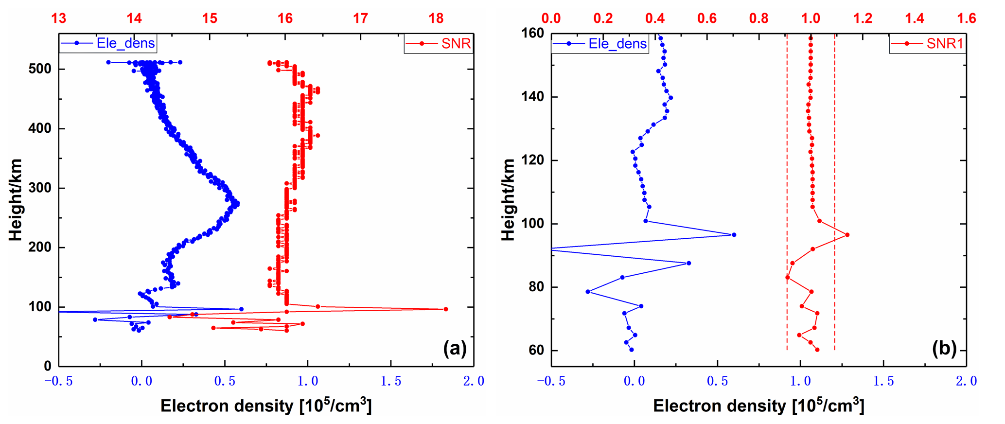
Figure 1 Schematic diagram of G06 single-layer E_s sounding. Panel (a) shows the electron density profile of the G06 occultation event and the SNR profile at 06:56 GPST on 14 August 2018. Panel (b) shows the electron density profile and normalized SNR profile within 60–160 km at the same time, and the red dotted line is the $\stackrel{\mathrm{‾}}{\text{SNR1}}\pm \mathrm{3}\text{std}$ boundary vertical.

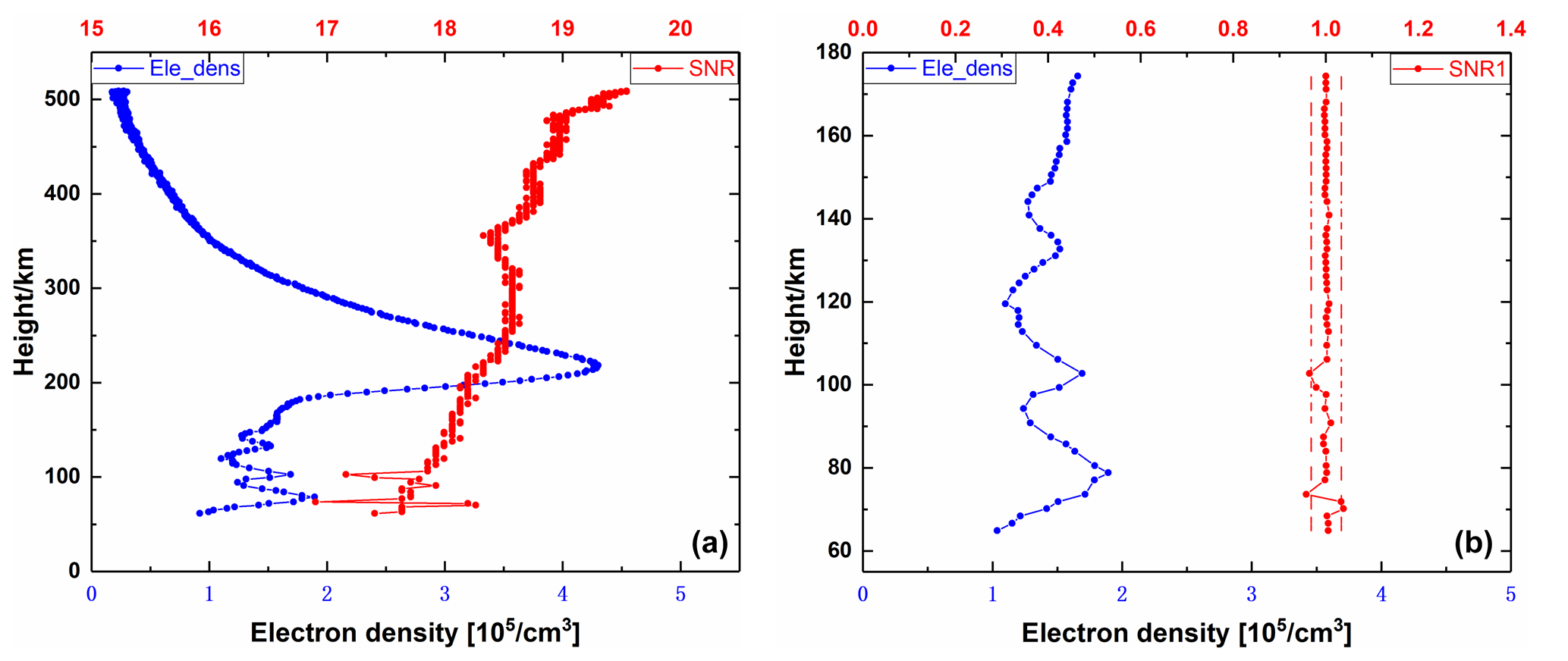
Figure 2 Schematic diagram of G17 multi-layer E_s sounding. Panel (a) shows the electron density profile of the G17 occultation event and the SNR profile at 20:58 GPST on 27 August 2018. Panel (b) shows the electron density profile and normalized SNR profile within 60–160 km at the same time, and the red dotted line is the $\stackrel{\mathrm{‾}}{\text{SNR1}}\pm \mathrm{3}\text{std}$ boundary vertical.

Under the assumptions of spherical symmetry (i.e., assuming only vertical electron density gradients), straight-line propagation, and Earth's spherical shape, we calculate the electron density profile by the occultation inversion algorithm, mainly referring to Lei et al. (2007). These assumptions, especially the assumption of spherical symmetry, are frequently not fully accurate for smaller-scale ionospheric phenomena, the calculated electron density values are not accurate and can only describe the approximate numerical distribution. Nevertheless, this study does not attempt to retrieve the absolute accurate electron density values of E_s, but it shows the electron density differences at E_s peaks compared to those electron density profiles without the E_s phenomenon. Our new criterion is developed to mainly use the normalized SNR to determine the E_s events; the electron density profile is only a reference to illustrate the effect of relatively higher electron density at E_s on the normalized SNR variation, and it is further verified that variance in SNR can be suggested to identify and sound sporadic E layers. There is a certain deviation in the low-altitude range by these assumptions, and the electron density calculated by inversion will also have an impact. Compared with the electron density itself, the signal-to-noise ratio is more sensitive to the electron density gradient; the SNR peak height does not fully correspond to the local peak of electron density. Therefore, it will affect the inversion height comparison.

3 Discussions on global E_s-event morphology

The GOR measurements of CSES from 1 March to 1 December in 2018 are used in the data analysis. With nearly 9 months of data from CSES, there are 104 531 and 12 642 electron density profiles obtained from GPS and BDS-2 data of CSES, respectively. The inversion algorithm is utilized based on the FUSING (FUSing IN Gnss) software (Shi et al., 2019; Zhao et al., 2019; Gu et al., 2020, 2021). Originally, the FUSING software is developed for high-precision real-time GNSS data processing and multi-sensor navigation, and now it can also be used for atmospheric modeling (Lou et al., 2019; Luo et al., 2020, 2021).

According to the orbital characteristics of CSES, the instruments of CSES mainly work in the region from 65^∘ S to 65^∘ N in latitude. For example, the Langmuir probe (LAP) detects the electron density in the space around CSES. As for the GNSS occultation receiver (GOR), it works in the region within the latitude of ±65^∘, but according to the principle of occultation inversion by the occultation receiver, the ionosphere that the GPS/BDS-2 satellite signals received by GOR pass through is globally distributed, and the tangent points of electron density profiles from CSES are globally distributed. Some scholars have given relevant global distribution results in their studies. Wang et al. (2019) showed the global distribution of the location of the tangent point of the maximum values in a profile of CSES from 90^∘ S to 90^∘ N. Lin et al. (2018) showed the distribution of the true NmF2, hmF2 and retrieved NmF2, hmF2 with respect to the local time and magnetic latitude from 90^∘ S to 90^∘ N, respectively. Cheng et al. (2018) showed that the global coverage of CSES GNSS radio occultation (GRO) events in more than 2 months and compared them with COSMIC observations; they concluded that both the CSES and COSMIC occultation data can realize global coverage, and they also showed the global distributions of layer F2 peak density and peak height derived from GRO from 90^∘ S to 90^∘ N.

Therefore, when we extract the electron density profiles corresponding to the tangent point and the SNR profile data, E_s occurrence rate sounded from CSES is globally distributed. The distribution of E_s occurrence rate is detailed in the four subsections below.

3.1 Distribution of E_s occurrence rate for seasons and altitude

The 9-month data have been divided into spring (March, April, and May), summer (June, July, and August), and autumn (September, October, and November). For each season, we use the altitude resolution of 1 km to count the number of occultation events which sound E_s events in each altitude interval. Due to the resolution of observation values, we do not distinguish the occultation events of sounding E_s in different layers. Considering the error caused by the integrity of the original observation data in different seasons and different days, we count the total number of days with observation data in each season, and we then calculate the ratio of the number of occultation events with E_s events in different height intervals to the total number of days in the season, that is, counting the number of occultation events with E_s events per day. Since CSES has both GPS and BDS-2 observations, we count the average number of daily occultation events which sound E_s events of different satellite systems. The results are as follows.

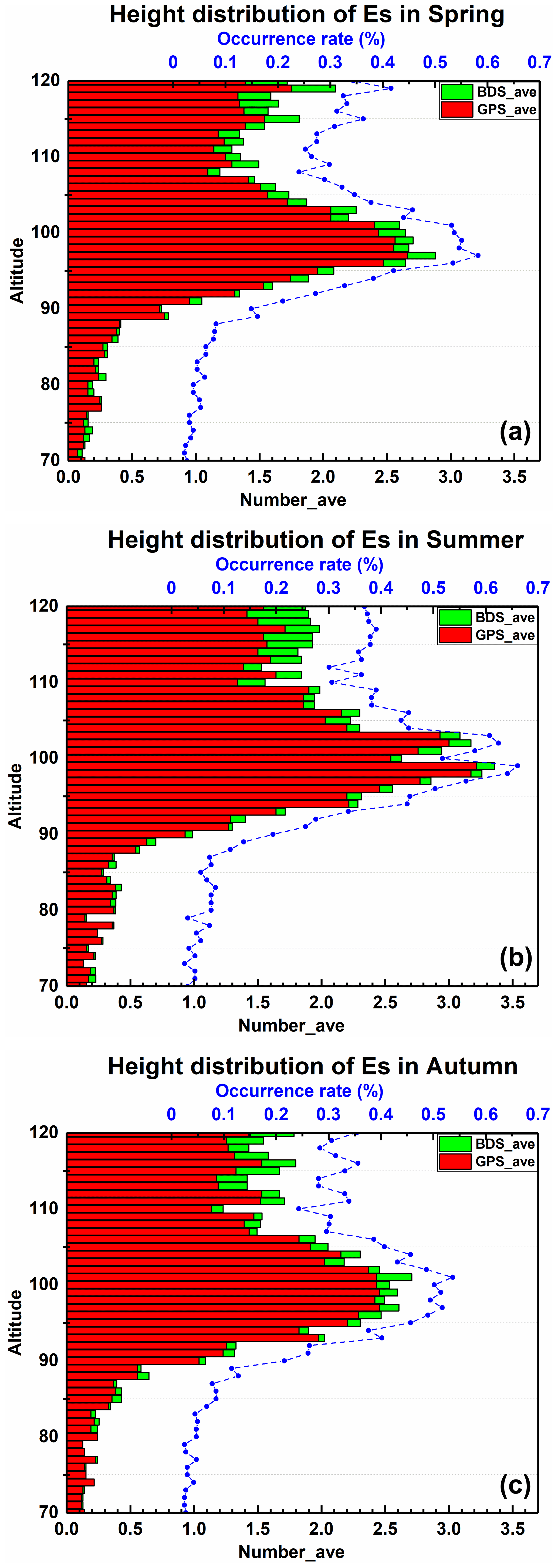
Figure 3 Height distribution of E_s average daily occurrence rate for three different seasons, Panels (a–c) are the results of spring, summer, and autumn, respectively. The blue dotted line diagram shows E_s occurrence rate, the red and green bar chart shows the number of occultation events with E_s events per day.

In Fig. 3 are the results of spring, summer, and autumn from top to bottom, respectively. Due to the lack of observation data of CSES for about 20 d in summer, it is not very appropriate to compare seasonal differences only by plotting the total number of occultation events with E_s. So, as shown in the blue dotted line diagram of Fig. 3, we also calculate the ratio of the number of occultation events with E_s events in different height intervals to the total number of occultation events in the season. It can be seen from Fig. 3 that the E_s average daily occurrence rate has obvious seasonal variation: the height of E_s occurrence in spring, summer, and autumn is mainly 90–110 km; the height with the largest daily average incidence of E_s in spring is 98 km, with a daily average of 2.88; the height with the largest daily average incidence in summer is 99 km, with a daily average of 3.36; and in autumn the height is 101 km, with a daily average of 2.71. The results show that significantly more E_s events appear above 110 km than below 90 km overall in the distribution of the three seasons. The reasons, firstly, are that there are less observation data of CSES at a lower altitude, and this situation is reflected in the blue dotted line of Fig. 3; secondly, due to the time resolution, some initial lower-altitude values are discarded when using the sliding window to calculate the SNR background trend term, and E_s occurring at a lower height is also discarded at the same time.

3.2 Distribution of global E_s occurrence rate for seasons

The global longitude and latitude regions are divided into grids with a resolution of $\mathrm{10}{}^{\circ }\times \mathrm{5}{}^{\circ }$. The number of occultation events in each grid and the number of occultation events with E_s events are counted, and the ratio of the number of occultation events with E_s to the total number of occultation observations is taken as the E_s occurrence frequency of the grid. In order to reduce the impact of accidental errors, we further optimized the statistical method, the E_s occurrence rate for the grid is calculated only when the number of occultation events in the grid is greater than 10. Finally, the global longitude–latitude distribution characteristics of E_s occurrence frequency in this season are obtained. The statistical results are as follows.

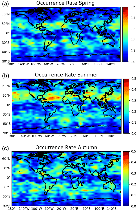
Figure 4 The geographical distribution of E_s occurrence rate for three different seasons in $\mathrm{5}{}^{\circ }\times \mathrm{10}{}^{\circ }$ geographic latitude/longitude grid. Panels (a–c) are the results of spring, summer, and autumn, respectively.

In Fig. 4 are the results of spring, summer, and autumn from top to bottom, respectively. In general, E_s preferably occurs at midlatitudes of the summer hemisphere. The overall occurrence frequency of global E_s in spring and autumn is lower than that in summer. This phenomenon may be due to the strong solar radiation in summer and the ionization of more metal atoms in the ionosphere, which increases the source of E_s and promotes the formation of E_s. Therefore, the occurrence rate in midlatitudes of the hemisphere in summer is higher than that in other latitudes (Chu et al., 2014). There is no significant difference in the frequency of E_s between the Northern Hemisphere and Southern Hemisphere in spring and autumn, and it shows an almost symmetrical trend along the equator. In spring and autumn, the direct point of the sun is near the equator. Because the magnetic line of force here is almost horizontal, it is difficult to form ion aggregation even if the ionization rate increases, so the occurrence rate is relatively high in the low-latitude area of the magnetic equator (Arras and Wickert, 2017; Xue et al., 2018). The E_s rates at polar regions are always low. We can also find an occurrence depression around the American area (the longitude sector of 70–120^∘ W) in the midlatitudes in summer, where the E_s occurrence rates were lower than anywhere else along the zone bands; this is consistent with the phenomenon found by Tsai et al. (2018).

3.3 Distribution of E_s occurrence rate for latitude and altitude

To comprehensively analyze the distribution of E_s incidence with latitude and altitude, the latitude–altitude region is divided into grids with a resolution of $\mathrm{10}{}^{\circ }\times \mathrm{1}$ km. Similarly, the ratio of the number of occultation events corresponding to E_s events in the grid to the total number of days with observed data in the season is calculated; the daily average number of E_s events is taken as the occurrence frequency of E_s for statistical analysis. The results are as follows.

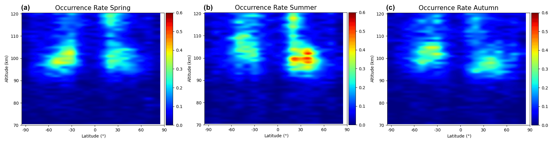
Figure 5 The distribution of E_s occurrence rate for three different seasons in $\mathrm{10}{}^{\circ }\times \mathrm{1}$ km geographic latitude/altitude grid, (a–c) are the results of spring, summer, and autumn, respectively.

In Fig. 5 are the results of spring, summer, and autumn from left to right, respectively. It can be seen from the figure that the incidence of E_s latitude altitude shows obvious seasonal changes. The incidence of E_s in summer in the Northern Hemisphere is significantly higher than that in spring and autumn in the same latitude range and height range. The latitude range of E_s high incidence is 20–50^∘ north–south latitude, mainly around 30^∘. The occurrence height of E_s is mainly concentrated in 90–110 km.

3.4 Distribution of E_s occurrence rate for local time and latitude

In order to comprehensively analyze the distribution of E_s incidence with local time and latitude, the local-time–latitude region is divided into grids with a resolution of $\mathrm{1}\mathrm{h}\times \mathrm{5}{}^{\circ }$. In order to exclude the effect of single-day observation integrity on the distribution of E_s incidence with local time, we use the ratio of the number of occultation events with E_s to the total number of occultation observations in the grid; at the same time, the E_s occurrence rate for the grid is calculated only when the number of occultation events in the grid is greater than 10 to reduce the impact of accidental errors. The results are as follows.

Figure 6 The distribution of E_s occurrence rate for three different seasons in $\mathrm{1}\mathrm{h}\times \mathrm{5}{}^{\circ }$ local time/geographic latitude grid, (a–c) are the results of spring, summer, and autumn, respectively.

In Fig. 6 are the results of spring, summer, and autumn from top to bottom, respectively. Maximum E_s occurrence is expected when the zonal wind shear, which is mainly produced by the semidiurnal tide in midlatitudes (Arras et al., 2009). At midlatitudes, the E_s activity is dominated primarily by a semidiurnal feature, which is generally believed to be induced by east–west zonal winds in terms of semidiurnal tides, especially in spring and summer (Whitehead, 1989; Chu et al., 2014). The semidiurnal tides generally start around 06:00 and 14:00 LT, continue for 14 h, and then fade out around 20:00 and 04:00 LT separately (Tsai et al., 2018). So, it can be seen from the figure that the incidence of E_s shows obvious local time changes, and the period of 14:00–20:00 LT is the high incidence period of E_s.

4 Experiments of comparing with ionosonde measurements

In this study, we choose a certain space-time matching criterion to obtain the pairs of the geometric altitudes of a sporadic E layer detected in CSES radio occultation profiles and the virtual heights of a sporadic E layer obtained by the ZLT ionosonde for confirming the derived sporadic E parameter in height. Luo et al. (2019) choose a certain space-time matching criterion to evaluate the quality of the electron density profile from the FY-3C mission with respect to the COSMIC mission. We modified their method to confirm the height of the derived sporadic E layer. We counted the data of Wuhan ZLT ionosonde from 1 March to 16 December in 2018 of the same period, and we extracted the h^′E_s data. The space-time matching criterion is quantified as the size of the space-time window centered on the position and occurrence time of the sporadic E layer obtained by the ZLT ionosonde. The sporadic E layer detected in CSES radio occultation profiles falling into the space-time window and the sporadic E layer obtained by the ZLT ionosonde constitute the pairs participating in the comparative analysis. Here the space-time window is denoted as (B, L, T), where B and L represent the size of space window along latitude and longitude, respectively; T represents the size of the time window.

Figure 7 An example of simultaneous detecting of E_s by CSES and ZLT ionosonde. Panel (a) shows the electron density profile and the SNR1 profile of G27 satellite at 17:42 GPST on 17 May 2018, as well as the electron density profile of ZLT ionosonde at 17:45 UTC on 17 May 2018. Panel (b) shows the electron density profile of ZLT ionosonde and the SNR1 profile in the range of 0–220 km. Panel (c) shows the ionogram image of Wuhan ZLT ionosonde.

In this study, considering that the temporal resolution of the ionosonde is 15 min, four different space-time matching criteria are proposed with the window as (10^∘, 10^∘, 7.5 min), (5^∘, 10^∘, 7.5 min), and (5^∘, 5^∘, 7.5 min), respectively. Among the other parameters, the height of the sporadic E layer is an important parameter of the derived sporadic E layer. Thus, the correlation coefficient (CC) is derived for determining the height of the sporadic E layer. The definition of the correlation coefficient is presented below.

$$\begin{array}{}\text{(5)}& \begin{array}{rl}& \text{CC}=\\ & {\displaystyle \frac{{\sum }_{i=\mathrm{1}}^N(X_i^{\mathrm{C}}\cdot X_i^{\mathrm{Z}})-\frac{\mathrm{1}}{N}{\sum }_{i=\mathrm{1}}^N{X}_i^{\mathrm{C}}{\sum }_{i=\mathrm{1}}^N{X}_i^{\mathrm{Z}}}{\sqrt{\left({\sum }_{i=\mathrm{1}}^N\right(X_i^{\mathrm{C}}{)}^{\mathrm{2}}-\frac{\mathrm{1}}{N}\left({\sum }_{i=\mathrm{1}}^N{X}_i^{\mathrm{C}}{)}^{\mathrm{2}}\right)\left({\sum }_{i=\mathrm{1}}^N\right(X_i^{\mathrm{Z}}{)}^{\mathrm{2}}-\frac{\mathrm{1}}{N}\left({\sum }_{i=\mathrm{1}}^N{X}_i^{\mathrm{Z}}{)}^{\mathrm{2}}\right)}}},\end{array}\end{array}$$

where N represents the total number of data pairs in the matching group under given spatiotemporal matching windows; $X_i^{\mathrm{C}}$ ($i=\mathrm{1},\mathrm{2},\mathrm{3},\mathrm{\dots },n$) represents the geometric altitudes of ith sporadic E layer detected in CSES radio occultation profiles; $X_i^{\mathrm{Z}}$ ($i=\mathrm{1},\mathrm{2},\mathrm{3},\mathrm{\dots },n$) represents the virtual heights of ith sporadic E layer obtained by the ZLT ionosonde.

The data of ionosonde are stored in SAO file format; this data file format contains different types of parameters, such as station information and detection time, ionospheric characteristic parameters for automatic measurements, echo traces (virtual height, amplitude, Doppler, frequency) at different height layers of the ionosphere (E, F1, F2), electron density profiles, virtual height and critical frequency of E_s trace, etc. For the SAO format description, we refer to https://ulcar.uml.edu/~iag/SAO-4.htm (last access: 1 March 2022). In order to facilitate the reading and use of data, SAOExplorer software (http://ulcar.uml.edu/SAO-X/SAO-X.html, last access: 1 March 2022) has been developed by the Center for Atmospheric Research at the University of Massachusetts Lowell, USA, to display and measure Digisonde ionospheric frequency maps observed by a series of ionospheric altimeters.

Figure 7 shows an example of simultaneously detecting E_s by CSES and ZLT ionosonde; the top left panel shows the electron density profile and the SNR1 profile of G27 satellite at 17:42 GPST on 17 May 2018, as well as the electron density profile of ZLT ionosonde at 17:45 UTC on 17 May 2018. The top right panel shows the electron density profile of ZLT ionosonde and the SNR1 profile in the range of 0–220 km. In the figure, the geodetic coordinates of E_s detected by CSES are (33.0^∘ N, 112.3^∘ E, 99.2 km), and the geodetic coordinates of E_s detected by ZLT are (30.5^∘ N, 114.4^∘ E, 102.5 km). The bottom panel shows the ionogram image of Wuhan ZLT ionosonde to show E_s situation. We can obtain the virtual height of E_s is 102.5 km, and we can also obtain the E_s layer critical frequency and frequency map at about 100 km.

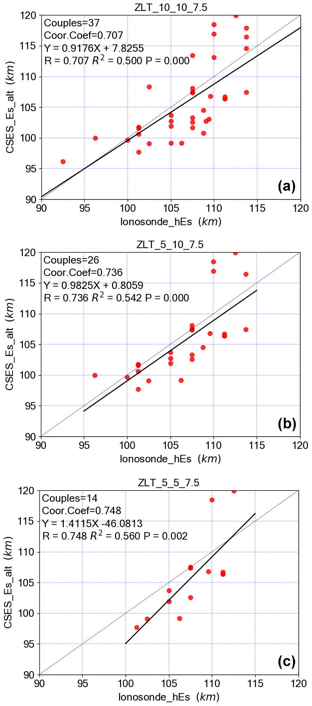
Figure 8 Comparison of the geometric altitudes of E_s detected in CSES radio occultation profiles and the virtual heights of E_s obtained by the ZLT ionosonde. Panels (a–c) are the results of space-time matching window (10^∘, 10^∘, 7.5 min), (5^∘, 10^∘, 7.5 min), and (5^∘, 5^∘, 7.5 min), respectively. The black solid line is the regression line.

Figure 8 presents the comparison of the geometric altitudes of a sporadic E layer detected in CSES radio occultation profiles and the virtual heights of a sporadic E layer obtained by the ZLT ionosonde. We also show the regression line as the solid black line and corresponding statistical coefficients in every subplot. These plots reveal that there is a good agreement between both parameters, which can also be seen from the high correlation larger than 0.7. The comparison among different windows concludes that the correlation increased slightly as a stricter space-time matching window was involved but with less pairs or couples. Compared with results from Arras and Wickert (2017), we also found a height offset between both measurement techniques mainly concentrated in 100–110 km of ionosonde altitude, and the calculation results of different space-time windows are different. The mean offset values in 100–110 km are 2.36, 2.25, and 2.90 km, which correspond to space-time matching windows of (10^∘, 10^∘, 7.5 min), (5^∘, 10^∘, 7.5 min), and (5^∘, 5^∘, 7.5 min), respectively. This may result from the different height parameters used for both techniques: the geometric heights provided by the RO technique and the virtual height which is influenced by the ionization below the sporadic E layer calculated from ionosonde recordings (Arras and Wickert, 2017).

5 Conclusions

The RO plays an important role in sounding of sporadic E layers. As China's first electromagnetic satellite, CSES has already provided service for more than 3 years up to now. In this study, the level-1 data of CSES and Wuhan ZLT ionosonde from 1 March to 1 December in 2018 are collected in sounding of sporadic E layers used to study the comparison of heights.

We calculate the geodetic longitude, latitude, and elevation of each occultation tangent point in the occultation inversion process and count the corresponding time information; we then extract the SNR data of L1 observations in the occultation inversion period. The occurrence of E_s is judged according to the judgment criterion of $|{\text{SNR1}}_i-\stackrel{\mathrm{‾}}{\text{SNR1}}|>\mathrm{3}\text{std}$. Single layer or multi-layer E_s is judged according to the number of data whose sequence meets the judgment criterion. Combined with the electron density profile of occultation inversion, the correctness of our E_s detection algorithm is verified.

According to the E_s results we detected, we drew distributions of E_s occurrence rate for seasons and altitude, as well as distribution of global E_s occurrence rate for seasons. It is concluded that the occurrence height of E_s is mainly located at 90–110 km, and there are obvious seasonal and latitudinal changes in the occurrence rate of E_s. There is no significant difference in the occurrence frequency of E_s in the Northern Hemisphere and Southern Hemisphere in spring and autumn, and it is almost symmetrical along the equator. Summer in the Northern Hemisphere is the time period of high incidence of E_s, and the latitude range of high incidence of E_s is 20–50^∘ in the northern and southern latitudes, mainly around 30^∘. The period of 14:00–20:00 LT is the high incidence period of E_s.

Finally, the comparison of the geometric altitudes of sporadic E layers detected in CSES radio occultation profiles and the virtual heights of sporadic E layers obtained by the ZLT ionosonde was carried out with different space-time matching window, i.e., (10^∘, 10^∘, 7.5 min), (5^∘, 10^∘, 7.5 min), and (5^∘, 5^∘, 7.5 min). For these three windows, the number of CSES matched pairs was 37, 26, and 14, respectively. The correlation coefficients of altitudes were 0.707, 0.736, and 0.748, respectively. The comparison of E_s altitudes from RO profiles with those from coinciding ground-based ionosonde measurements revealed a large correspondence between both measurement techniques.