the Creative Commons Attribution 4.0 License.
the Creative Commons Attribution 4.0 License.
 | 15 Jun 2022
Finite-difference time-domain analysis of ELF radio wave propagation in the spherical Earth–ionosphere waveguide and its validation based on analytical solutions
Volodymyr Marchenko
Andrzej Kulak
Janusz Mlynarczyk
The finite-difference time-domain (FDTD) model of electromagnetic wave propagation in the Earth–ionosphere cavity was developed under assumption of an axisymmetric system, solving the reduced Maxwell equations in a 2D spherical coordinate system. The model was validated on different conductivity profiles for the electric and magnetic field components for various locations on Earth along the meridian. The characteristic electric and magnetic altitudes, phase velocity, and attenuation rate were calculated. We compared the results of numerical and analytical calculations and found good agreement between them. The undertaken FDTD modeling enables us to analyze the Schumann resonances and the propagation of individual lightning discharges occurring at various distances from the receiver. The developed model is particularly useful when analyzing ELF measurements.
- Article
(552 KB) - Full-text XML
- BibTeX
- EndNote


The finite-difference time-domain (FDTD) model is a numerical analysis technique based on time-dependent differential Maxwell equations. It was originally developed for Cartesian coordinate system, but after elaboration of the code for spherical coordinates, it found applications in studies of extremely low frequency (ELF) and very low frequency (VLF) radio wave propagation in the Earth–ionosphere waveguide (Holland, 1983; Hayakawa and Otsuyama, 2002; Simpson and Taflove, 2002; Otsuyama et al., 2003; Yang and Pasko, 2005; Yu et al., 2012; Samimi et al., 2015). Similar analysis can be performed for Mars and other planets (Soriano et al., 2007; Navarro et al., 2007; Yang et al., 2006; Navarro et al., 2008).
When a small part of the Earth–ionosphere cavity needs to be analyzed, a local volume can be divided into FDTD grid in 2D cylindrical (Cummer, 2000; Hu and Cummer, 2006; Marshall, 2012; Qin et al., 2019), or 3D Cartesian coordinate systems (Araki et al., 2018; Suzuki et al., 2016). It facilitates taking into account some complex inhomogeneities and ionospheric anisotropy in the analysis of ELF–VLF radio waves.
FDTD modeling in 3D Cartesian coordinates system was used for verification of Wait's and Cooray–Rubinstein's analytical formulas, describing lightning-radiated electric and magnetic fields for a mixed propagation path (vertically stratified conductivity), and for the fractal rough ground surface (Zhang et al., 2012a, b; Li et al., 2013, 2014).
The analysis of propagation over a mountainous terrain was performed in a 2D axial symmetric model (Li et al., 2016), which was further developed into an FDTD model in a 2D spherical axisymmetric coordinate system (Li et al., 2019). In such modeling the authors have investigated the effect of the Earth–ionosphere waveguide structure and medium parameters, including the effect of the ionospheric cold plasma characteristics, the effect of the Earth's curvature, and the propagation effects over a mountainous terrain.
A full-wave finite element method was used to calculate electromagnetic fields in a horizontally stratified ionosphere treated as a magnetized plasma (Lehtinen and Inan, 2008). The authors have implemented the source currents with arbitrary vertical and horizontal distributions. The electromagnetic field was calculated both in the Earth–ionosphere waveguide and in the ionosphere as an upward propagating whistler mode wave. This model was used to simulate trans-ionospheric propagation of VLF electromagnetic waves from ground-based transmitters up to satellite altitudes (Lehtinen and Inan, 2009).
In a recent paper by Nickolaenko et al. (2021) the propagation of natural wide-band pulsed radio signals in the spherical Earth–ionosphere cavity is numerically simulated. Applying the realistic vertical profiles of ionospheric conductivity, those authors have obtained ELF–VLF propagation parameters by the full wave solution in the form of Riccati differential equation. Using the day and night ionosphere models, the correspondent parameters were calculated for different source–observer distances.
The influence of ionospheric disturbances on the Schumann resonances was analyzed using the 3D FDTD model in Navarro et al. (2008). The authors estimated the role of day–night asymmetry, polar non-uniformities associated to solar proton events, and X-ray bursts.
Few other numerical approaches were used for the estimation of the parameters of the Earth–ionosphere resonator, like the two-dimensional telegraph equation (TDTE) in a two-dimensional spherical transmission line model of the Earth–ionosphere cavity (Kulak et al., 2003; Prácser et al., 2019; Bozóki et al., 2019) and the transmission line matrix (TLM) numerical method in Cartesian and spherical coordinate systems (Morente et al., 2003; Toledo-Redondo et al., 2016).
Besides the Schumann resonances, another important aspect of ELF studies concerns propagation of ELF waves generated by individual lightning discharges, including Q-burst phenomena (Ogawa et al., 1967). Their waveforms observed at large distance from the source are significantly influenced by the dispersive properties of the Earth–ionosphere waveguide and the round-the-world propagation. Inverse solutions in such cases should take into account full non-uniform solutions of the Maxwell equations. This is particularly important for lighting discharges that have a long continuing current phase or are associated with transient luminous events (TLE) when they occur at large distance from the receiver.
The development of an FDTD model was motivated by our ELF systems: the World ELF Radiolocation Array (WERA) (Kulak et al., 2014) and a new European ELF radiolocation system (EERS) (Mlynarczyk et al., 2018), which are operating in the ELF range, as well as for possible stations on Mars.
In this paper, we present an FDTD uniform model in 2D spherical coordinates and introduce a new approach for validation the FDTD models by introducing computation of complex altitudes of the Earth–ionosphere waveguide, which allows us to compare numerical results with two-scale-height analytical solutions. We also infer the resonance frequencies of Earth–ionosphere waveguides for various conductivity profiles using the decomposition method (Kulak et al., 2006).
We have created the FDTD model following the ideas which were originally proposed by Holland (1983) and developed in further studies (Hayakawa and Otsuyama, 2002; Otsuyama et al., 2003; Yang and Pasko, 2005; Navarro et al., 2007; Yang et al., 2006; Navarro et al., 2008). We chose a spherical coordinate system to be able to study the wave's propagation in the Earth–ionosphere cavity and analyze the Schumann resonances.
Since in the present work we did not intend to study the azimuthal dependence of propagation parameters, we reduced a 3D system of Maxwell equations to a 2D axisymmetric system. It allowed us to significantly decrease the required computational power and enabled longer simulation times, which leads to a better frequency resolution (up to df = 0.01 Hz).
2.1 Updated equations
In the case of spherical systems, assuming no dependence on the ϕ coordinate, the system of six Maxwell equations in 3D spherical coordinates (r, θ, ϕ) can be reduced to 2D spherical systems (r, θ) with three equations for Er, Eθ, and Hϕ field components (Holland, 1983; Inan and Marshall, 2011):
where σ=σ(r) is the conductivity profile of Earth–ionosphere cavity, and ε0 and μ0 are the vacuum permittivity and permeability, respectively.
These equations were discretized using central-difference approximations to the space and time partial derivatives. The resulting finite-difference equations are solved in a leapfrog manner: the electric field vector components in a volume of space are solved at a given instant in time; then the magnetic field vector components in the same spatial volume are solved at the next instant in time and the process is repeated over and over again until the desired transient or steady-state electromagnetic field behavior is fully evolved (Inan and Marshall, 2011). So the update equations for Er, Eθ, and Hϕ are the following (Holland, 1983):
where Δt is the time step, Δr and Δθ are the sizes of grid cell in r and θ coordinates, respectively, , , θj=jΔθ, , and R0 is the mean of Earth's radius. Superscript n signifies that the quantities are to be evaluated at time t=nΔt, and i,j represent the point (r=iΔr, θ=jΔθ) in the spherical grid. The half time steps indicate that the electric and magnetic fields are calculated alternately.
The updated equation for Er cannot be applied for poles (where θ=0 and θ=π) because of sin θ in the denominator. To solve this singularity problem the Holland's approach was used (Holland, 1983). Namely, for the poles the integral form of the curl equation with a small contour around the poles was applied, which leads to updated equations for poles without singularities. After that, the updated equation for θ=0∘ takes the following form (Holland, 1983):
And for θ=180∘:
where , , and Nθ is the number of grid cells in the θ direction.
2.2 Mesh
The size of grid cell (in the r and θ directions) is defined by the desired range of frequencies, which are going to be analyzed. For the present analysis we used Δr=1 km and Δθ=0.1∘, which lets us analyze frequencies up to 1 kHz. The ground was modeled as a perfect electric conductor. Also, the upper boundary Rmax for the model is a perfect conductor, but it was placed at high enough altitude to make sure that there would be no reflection of the waves from this boundary.
The total simulation time is defined by the desired frequency resolution of FFT ( Hz). The time step is defined by the stability of Courant's criterion , where c is the speed of light and a is Earth's radius (Inan and Marshall, 2011). In order to get sufficient frequency resolution (in our case it is 0.01 Hz, to be able to study the differences between different models), we have conducted the FDTD simulation up to 100 s.
2.3 Source
In order to analyze the propagation of electromagnetic waves originating from lightning discharges, one has to use the source model with similar characteristics to real lightning discharge. We used the time profile of lightning discharge proposed in Kulak et al. (2010) and Rakov (2007), which has a flat spectrum in a wide frequency range. But taking into account the restrictions connected with the FDTD computational grid, we had to modify the source: the highest frequency (or smallest wavelength) is defined by the cell size, and according to the generally accepted rule the smallest wavelength should be at least 10–20 times larger than the cell size. Therefore, the source has to be filtered with a loss-pass filter in order to remove frequency components that do not fit the size of the computational cell.
Also, it should be noted that if the source contains the direct current (DC) in its spectrum, it can introduce artifacts, which are not physical (Li et al., 2013). Therefore, additional filtering has to be used for the lowest frequencies by a high-pass filter. For such filtering we have used a fifth-order Butterworth low-pass filter with a cutoff frequency of 300 Hz and a third-order Butterworth high-pass filter with a cutoff frequency of 2 Hz. The final spectrum of this modified source is almost flat in the range 5–100 Hz but decreases rapidly for f<3 and f>1000 Hz.
We placed the source in the FDTD grid at the pole (θ=0∘) in radial direction in nodes with i = 0–6, which corresponds to the source length L=6 km. Also, for the implementation of the source into the FDTD grid we took into account the lightning stroke speed, and for our analysis we used v=108 m s−1 (Rakov, 2007). We assumed a cloud-to-ground (CG) discharge and implemented it according to the time delay between adjacent nodes in the source.
The main purpose of the current work is the analysis of resonance phenomena in the Earth–ionosphere cavity. In order to validate the developed FDTD model, we analyzed several configurations of spherical waveguide with known analytical solutions and compared them with our FDTD results. We compared the resonance frequencies for them in relative and absolute units.
3.1 Lossless spherical waveguide
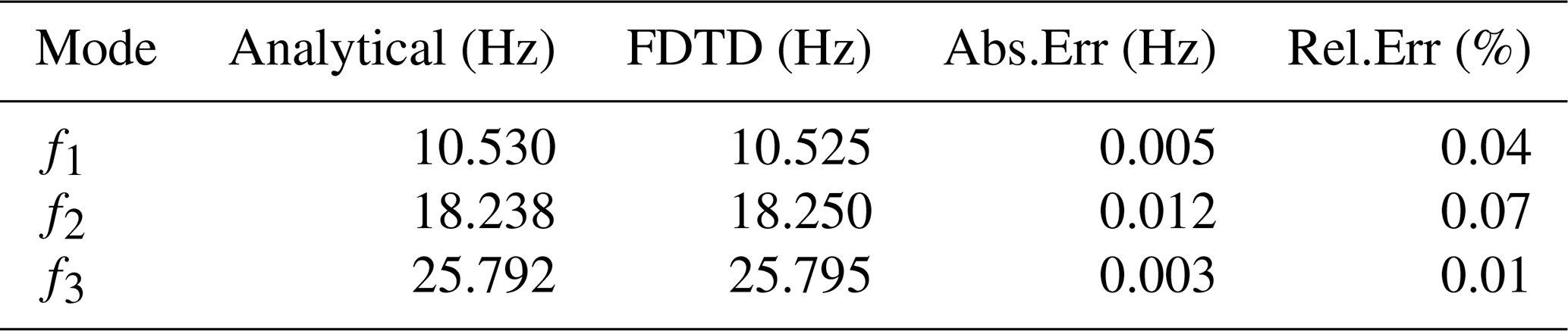
The first model for testing was a lossless spherical waveguide with perfect electric conductors at the ground and the upper boundary. The distance between the conductors was set to h=74 km. The precise theoretical resonance frequencies for such a waveguide for a given height are presented by the equation , where c is the speed of light, a is Earth's radius, and n is the mode of resonance frequency (Bliokh et al., 1977). A comparison of analytical and numerical results for such a model is presented in Table 1. The results of the FDTD analysis for this model are shown at Fig. 1.
Table 1Comparison of resonance frequencies obtained analytically and numerically for a lossless spherical waveguide.
3.2 Spherical waveguide with a conducting layer
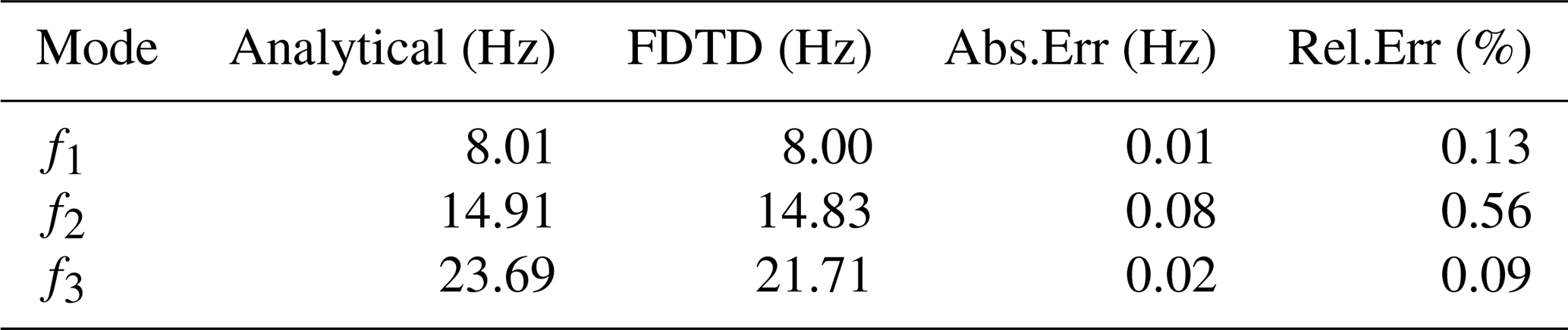
A more complicated model for testing had a perfect conductor at the ground and a constant conductivity of S m−1 above 70 km. The analytical solutions for this model were obtained by Kulak and Mlynarczyk (2013). A comparison of analytical and numerical results for such a model is presented in Table 2. The results of the FDTD analysis for this model are shown at Fig. 1.
Table 2Comparison of resonance frequencies obtained analytically and numerically for a spherical waveguide with a conducting layer above 70 km.
3.3 Two-layered spherical waveguide
The third model for testing was a two-layered model with a perfect conductor at the ground, a constant conductivity of S m−1 at altitudes between 70 and 110 km, and a constant conductivity of S m−1 above 110 km. The analytical results for such a model can be found in Kulak et al. (2013), which deals with multi-layer waveguides. A comparison of analytical and numerical results for this model is presented in Table 3. The results of the FDTD analysis for this model are shown at Fig. 1.
Table 3Comparison of resonance frequencies obtained analytically and numerically for a two-layered spherical waveguide.
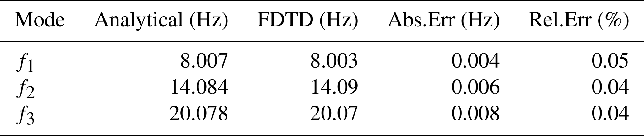
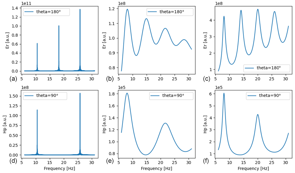
Figure 1The FDTD spectrum for spherical waveguide with a lossless perfect cavity (a, d), one conducting layer (b, e), and two layers (c, f) for an electric component at 90∘ and a magnetic component at 180∘.
The next validation of our FDTD model was done for a realistic atmospheric conductivity profile (Kudintseva et al., 2016; Nickolaenko et al., 2016). We did not take into account the influence of Earth's magnetic field. The resulting anisotropy of the conductivity has little influence in the analyzed frequency range (i.e., 0–100 Hz). As shown in Yu et al. (2012), the anisotropy has a more significant influence at higher frequencies.
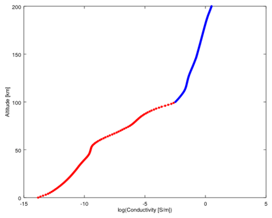
Figure 2A realistic conductivity profile up to 200 km obtained by combining the profile from Kudintseva et al. (2016) (red part) and an IRI profile (blue part).
For the lower part of the atmosphere (0–100 km) we used a conductivity profile recently proposed by Kudintseva et al. (2016). Since the upper boundary of this profile has the conductivity much below 1 S m−1, which is not enough to attenuate the ELF waves, reflections in the FDTD grid would occur from the perfect electric conductor (PEC) at its upper boundary. To avoid reflections and let the waves attenuate gradually at high altitudes, we extended this profile up to 200 km using the IRI (International Reference Ionosphere) model. We chose it in such a way that the combined profile would be smooth (Fig. 2). The required IRI profile was found on 22 January 2006, at 06:00 UT, for the location typical for mid-latitudes (49∘ N, 23∘ E). The results of the FDTD analysis for this model are shown at Fig. 3.
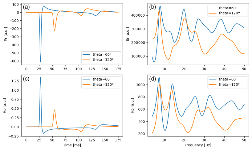
Figure 3The results of the FDTD analysis are shown, which were obtained using the realistic conductivity profile described in Fig. 2. The solutions for the electric component Er (a, b) and the magnetic component Hϕ (c, d) are shown in the time domain (a, c) and frequency domain (b, d). Each plot contains the results for two probe positions (60 and 120∘).
4.1 Characteristic electric and magnetic altitudes
To be able to compare the numerical results with the analytical solutions, we have extracted the complex characteristic electric and magnetic altitudes from the FDTD model. The corresponding altitudes can be extracted using their definition (Mushtak and Williams, 2002; Kirillov, 1993):
where N is the number of radial nodes, and are the complex field values at the radial node i for a given frequency, and , are the values of these fields at the ground level.

Figure 4Real and imaginary parts of characteristic electric and magnetic altitudes obtained analytically (denoted by “A”) and from the FDTD model (denoted by “N”).
The complex electric altitude can also be expressed using the conductivity profile by the analytical equation in a normalized form (Mushtak and Williams, 2002):
where and the characteristic conductivity value for electric altitude is , and ω=2πf.
Assuming a similar dependence for complex magnetic altitude and taking into account that the characteristic conductivity value for magnetic altitude is (Greifinger and Greifinger, 1978)
where the scale height , we can write a similar equation for the complex magnetic altitude:
where . We compared the characteristic electric and magnetic altitudes calculated analytically from Eqs. (11) and (12) with the FDTD results calculated from Eqs. (9) and (10). The results are presented in Fig. 4.
4.2 Propagation parameters
We calculated the phase velocity Vph and the attenuation rate α using two different methods: numerical and analytical. Analytically the propagation parameters can be calculated using the conductivity profile and electric and magnetic altitudes given by Eqs. (11) and (12), through the following relationship (Kulak and Mlynarczyk, 2011):
where .
In the case of numerical calculations those parameters were obtained by two approaches: (a) similarly to analytical as described above but using electric and magnetic altitudes from FDTD model by Eqs. (9) and (10); and (b) directly from the spectra of electric and magnetic field components. Assuming that in our coordinate system the wave propagates in the θ direction, the following relationship can be written in the frequency domain:
where the ratio of magnetic field complex amplitudes are calculated for two probes “1” and “2” which are located at distances ρ1 and ρ2 from the source, respectively. In this equation the propagation constant , where α is the attenuation rate (in units Np m−1) and β is the phase constant, so the phase velocity is . For further convenient usage we convert the units of attenuation rate to dB Mm−1. A similar relationship to Eq. (15) but for electric field components can be written as well.
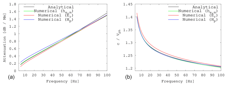
Figure 5The attenuation rate and phase velocity that was calculated analytically and numerically. Using numerical FDTD calculations those parameters were obtained by two approaches: (a) using electric and magnetic altitudes from FDTD by Eqs. (9) and (10); and (b) directly from the spectra of electric and magnetic field components following Eq. (15), where we used probes located at 80 and 90∘.
We should note that Eq. (15) for and spectra calculated in a closed cavity gives non-monotonic behavior of propagation parameters. This is caused by superposition of wave attenuation along meridian and different amplitudes of the Schumann resonances for different source–observer distances. One possible solution for removing the influence of Schumann resonances is to implement a perfectly matched layer (PML) along the θ direction. However, we solved this problem in a different way, transforming the Maxwell equations at angle θ>90∘ from spherical coordinates to plane equations, changing the behavior of equations from “closed” to “open”. In this case the waves are unable to propagate around Earth and therefore the Schumann resonance does not occur. The calculated propagation parameters from all the methods listed above are presented in Fig. 5.
4.3 Spectral decomposition method
As an additional validation we applied the spectral decomposition technique to Schumann resonance power spectra. Figure 6 presents the resonance frequencies obtained from the spectra measured at different distance from the source, and the decomposed frequencies that do not depend on the source–observer distance. Following the decomposition algorithm (Kulak et al., 2006; Dyrda et al., 2014), the spectrum is approximated by the function
where W(f) is the signal power spectrum, s is the white noise component, is the color noise term, pk is the power parameter of the kth resonance peak, ek is the peak asymmetry parameter, fk is the resonance frequency, and gk is the resonant mode half-width parameter. Fitting this function to the FDTD spectra allows us to extract the resonance frequencies fk of the cavity, which are not equal to Schumann resonance frequencies. The Schumann resonance frequencies obtained from the spectra depend on the distance from the source and represent the superposition of standing and traveling waves (Kulak et al., 2006). To analyze the standing waves separately and reveal the properties of the resonant cavity, we use the spectral decomposition method described in Kulak et al. (2006) and Dyrda et al. (2015). After applying this method, the resonance frequencies become independent of the source–observer distance (see details in Kulak et al., 2006 and Dyrda et al., 2015). The decomposition method shows that the solutions for the electric field are symmetric at θ=180∘ because the traveling waves cancel each other out and only the standing waves remain. Therefore, the resonant peaks measured from the spectrum at θ=180∘ for the electric field component () represent the resonance frequency of the cavity, and they are in agreement with the decomposed frequencies.
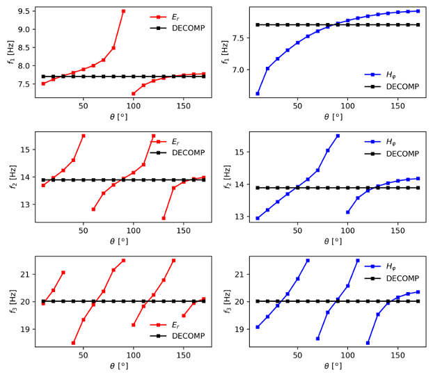
Figure 6The Schumann resonance frequencies of the first three modes obtained at different source–observer distances and the resonance frequencies of the cavity obtained by the decomposition method (Kulak et al., 2006).
4.4 Resonance frequencies of the Earth–ionosphere cavity
The resonance frequencies of the Earth–ionosphere cavity for a given conductivity profile can be calculated by different approaches, and the consistency between them can be considered as an additional validation of the model. We have considered the followings ways to calculate the resonant frequencies:
-
Analytically using the conductivity profile. The resonance frequencies in this approach are calculated by solving the following equation (Mushtak and Williams, 2002; Galejs, 1972):
where depending on the characteristic complex altitudes, which are discussed in Sect. 4.1;
-
Numerically from the FDTD model using Eq. (17). We denote these resonant frequencies by ;
-
Using FDTD spectra for (see Sect. 4.3 for details). We denote these frequencies by ;
-
Using the spectral decomposition method (see Sect. 4.3 for a description). We denote these resonant frequencies by .
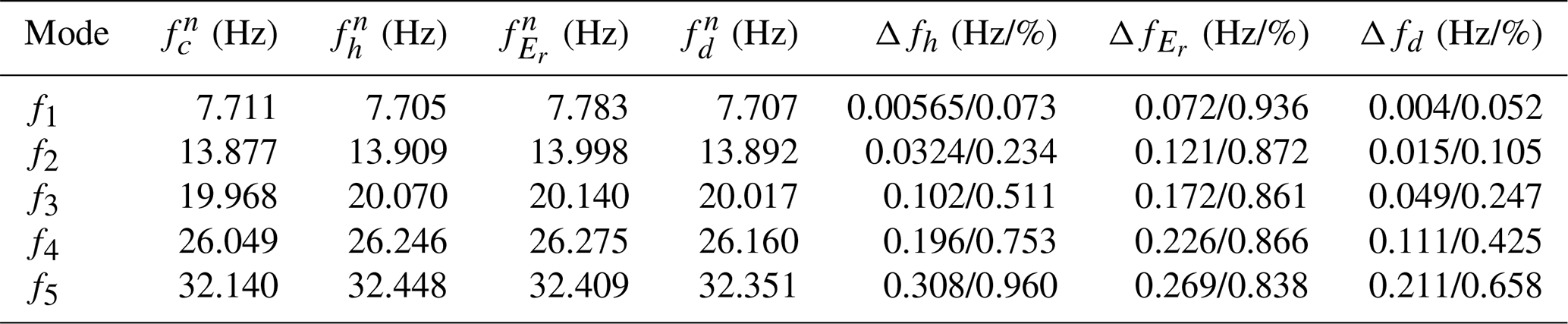
The obtained resonance frequencies are presented in Table 4. We compared these frequencies with the analytical results, and the absolute and relative differences are presented in the corresponding columns.
Table 4Resonance frequencies for the conductivity profile shown in Fig. 2 calculated by different approaches described in Sect. 4, and the relative error obtained by comparison with the analytically obtained resonance frequency.
In this study, we used new methods for validation of numerical simulation:
-
We compared the complex electric and magnetic altitudes of the Earth–ionosphere waveguide, referring to two-dimensional formalism of electromagnetic wave propagation in the Earth–ionosphere cavity. The two complex altitudes were calculated numerically directly from their definitions as given in Eqs. (9) and (10), making use of radial field solutions E(r) and H(r). These altitudes were directly compared with the altitudes obtained with analytical formulas as given in Eqs. (11) and (12) for the same conductivity profile of the atmosphere. This allowed us to fully validate the simulation results.
-
We determined the resonance frequencies of the cavity using the decomposition of power spectra described by Eq. (16). The resonance frequencies cannot be directly determined from the spectra obtained using FDTD, because the field generated by the source in each point of the cavity is a superposition of traveling waves propagating directly from the source and the resonance field resulting from the interference of waves propagating around the world. The resulting Schumann resonance frequencies depend on the source–observer distance (Kulak et al., 2006). Close to the source, where the amplitudes of the traveling waves are significant, the resonance frequencies differ by several percent from the Schumann resonance frequencies obtained by FDTD. With the use of the decomposition method we determined the intrinsic resonance frequencies of the cavity, which are the same at each location, independently from the distance to the source. This enabled us to compare the resonance frequencies obtained from the numerical simulation with the frequencies determined directly from analytical Eq. (9). This method should be recommended as a reference for validation of numerical models.
-
We determined the propagation parameters of the Earth–ionosphere waveguide using the FDTD results in two different points of the great circle. Equation (15) allowed us to determine the phase velocity and the attenuation rate of the Earth–ionosphere cavity. We compared them with the results obtained from analytical Eqs. (13) and (14).
In this paper, we analyzed the solutions of Maxwell's equations obtained by the FDTD method for an axisymmetric uniform Earth–ionosphere cavity. We analyzed the propagation of radio waves generated by a short current impulse.
We constructed an FDTD model in axisymmetric spherical coordinate system with the source implemented at the pole. We took into account the finite speed of lightning discharge and implemented the time delay between adjacent nodes in the source.
We validated the model thoroughly, comparing the resonance frequencies, propagation parameters, and electric and magnetic characteristic altitudes. Since the conductivity profile of the atmosphere has a significant influence on radio wave propagation and resonance frequencies, we validated our model for various conductivity profiles.
We paid close attention to the verification of accuracy of the FDTD computations and used a new approach for that purpose. It is based on 2D formalism of wave propagation in the Earth–ionosphere cavity and it allowed us to compare the numerical and the analytical solutions. In this approach, the propagation parameters of the Earth–ionosphere waveguide are defined using the electric and magnetic altitudes. These altitudes can be calculated directly when the vertical conductivity profile of the atmosphere is known.
The obtained analytical solutions were used as reference and compared with the numerical results. First, we compared the solutions for three cases: a perfect cavity, a cavity formed by a perfect ground and a homogenous conducing layer, and a cavity formed by a perfect ground and two-layered upper boundary of the waveguide. As a measure of error between the models, we took the difference between the first three resonance frequencies. The analytical and numerical solutions were in agreement (Tables 1–3). Next, we compared the results for a continuous conductivity profile. We built a realistic conductivity model of which the lower part was based on a recently proposed conductivity profile and the upper part was based on an IRI model. We obtained good agreement between the resonance frequencies of the cavity and the observed Schumann resonance frequencies (Table 4).
Using our FDTD model, we also calculated the spectral dependence of the phase velocity and the attenuation rate. We showed that the analytical and numerical models are in agreement.
The presented model can be used for studying the propagation of ELF electromagnetic waves generated by lighting discharges of various types with the round-the-world propagation taken into account.
The software code used in this paper can be accessed by https://doi.org/10.5281/zenodo.6628335 (Marchenko et al., 2022a).
The conductivity profile data used in this paper can be accessed by https://doi.org/10.5281/zenodo.6628304 (Marchenko et al., 2022b).
AK formulated the concept of the current research. VM wrote the FDTD code, the python scripts for the post-processing and visualization, contributed to the development of the analytical model used for the validation of the FDTD results in Sect. 4, and prepared the initial version of the manuscript. JM calculated the analytical results for the validation in Sect. 3 and participated in the preparation of the scripts for the post-processing of the FDTD results. All authors participated in the interpretation of the results and contributed to the final version of the paper.
The contact author has declared that neither they nor their co-authors have any competing interests.
Publisher’s note: Copernicus Publications remains neutral with regard to jurisdictional claims in published maps and institutional affiliations.
The numerical computations were done using the PL-Grid infrastructure. The present work was supported by the National Science Centre, Poland, under grants 2016/22/E/ST9/00061 (Volodymyr Marchenko), 2015/19/B/ST9/01710 (Andrzej Kulak), and 2015/19/B/ST10/01055 (Janusz Mlynarczyk).
This research has been supported by the National Science Centre, Poland (grant nos. 2016/22/E/ST9/00061, Volodymyr Marchenko; 2015/19/B/ST9/01710, Andrzej Kulak; and 2015/19/B/ST10/01055, Janusz Mlynarczyk).
This paper was edited by Keisuke Hosokawa and reviewed by Alexander P. Nickolaenko and one anonymous referee.
Araki, S., Nasu, Y., Baba, Y., Rakov, V. A., Saito, M., and Miki, T.: 3-D Finite Difference Time Domain Simulation of Lightning Strikes to the 634-m Tokyo Skytree, Geophys. Res. Lett., 45, 9267–9274, https://doi.org/10.1029/2018GL078214, 2018.
Bliokh, P. V., Galyuk, Yu. P., Hunninen, E. M., Nickolaenko, A. P., and Rabinovich, L. M.: On resonance phenomena in the Earth-ionosphere cavity, Radiofizika, XX, 501, 1977 (in Russian).
Bozóki, T., Prácser, E., Sátori, G., Dálya, G., Kapás, K., and Takátsy, J.: Modeling Schumann resonances with schupy, J. Atmos. Sol.-Terr. Phy., 196, 105144, https://doi.org/10.1016/j.jastp.2019.105144, 2019.
Cummer, S. A.: Modeling electromagnetic propagation in the Earth-ionosphere waveguide, IEEE T. Antennas Propag., 48, 1420–1429, https://doi.org/10.1109/8.898776, 2000.
Dyrda, D., Kulak, A., Mlynarczyk, J., Ostrowski, M., Kubisz, J., Michalec, A., and Nieckarz, Z.: Application of the Schumann resonance spectral decomposition in characterizing the main African thunderstorm center, J. Geophys. Res.-Atmos., 119, 13338–13349, 2014.
Dyrda, M., Kulak, A., Mlynarczyk, J., and Ostrowski, M.: Novel analysis of a sudden ionospheric disturbance using Schumann resonance measurements, J. Geophys. Res.-Space, 120, 2255–2262, https://doi.org/10.1002/2014JA020854, 2015.
Galejs, J.: Terrestrial Propagation of Long Electromagnetic Waves, edited by: Cullen, A. L., Fock, V. A., and Wait, J. R., Pergamon, New York, ISBN 978-14-8315-956-0, 1972.
Greifinger, C. and Greifinger, P.: Approximate method determining eigenvalues earth-ionosphere for ELF in the waveguide, Radio Sci., 13, 831–837, 1978.
Hayakawa, M. and Otsuyama, T.: FDTD analysis of ELF wave propagation in inhomogeneous subionospheric waveguide models, Appl. Computational Electromagnetics Soc. J., 17, 239–244, 2002.
Holland, R.: THREDS: A finite-difference time-domain EMP code in 3D spherical coordinates, IEEE T. Nucl. Sci., NS-30, 4592–4595, 1983.
Hu, W. and Cummer, S. A.: An FDTD model for low and high altitude lightning-generated EM fields, IEEE T. Antennas Propag., 54, 1513–1522, 2006.
Inan, U. S. and Marshall, R. A.: Numerical Electromagnetics: The FDTD Method, Cambridge University Press, ISBN 978-05-2119-069-5, 2011.
Kirillov, V. V.: Parameters of the earth-ionosphere waveguide at ELF, Probl. Diffr. Wave Propagat., 25, 1993 (in Russian).
Kudintseva, I. G., Nickolaenko, A. P., Rycroft, M. J., and Odzimek, A.: AC and DC global electric circuit properties and the height profile of atmospheric conductivity, Ann. Geophys., 25, 35–52, 2016.
Kulak, A. and Mlynarczyk, J.: A new technique for reconstruction of the current moment waveform related to a gigantic jet from the magnetic field component recorded by an ELF station, Radio Sci., 46, RS2016, https://doi.org/10.1029/2010RS004475, 2011.
Kulak, A. and Mlynarczyk, J.: ELF Propagation Parameters for the Ground-Ionosphere Waveguide With Finite Ground Conductivity, IEEE T. Antennas Propag., 61, 2269–2275, https://doi.org/10.1109/TAP.2012.2227445, 2013.
Kulak, A., Zieba, S., Micek, S., and Nieckarz, Z.: Solar variations in extremely low frequency propagation parameters: 1. A two-dimensional telegraph equation (TDTE) model of ELF propagation and fundamental parameters of Schumann resonances, J. Geophys. Res.-Space, 108, 1270, https://doi.org/10.1029/2002JA009304, 2003.
Kulak, A., Mlynarczyk, J., Zieba, S., Micek, S., and Nieckarz, Z.: Studies of ELF propagation in the spherical shell cavity using a field decomposition method based on asymmetry of Schumann resonance curves, J. Geophys. Res., 111, A10304, https://doi.org/10.1029/2005JA011429, 2006.
Kulak, A., Nieckarz, Z., and Zieba, S.: Analytical description of ELF transients produced by cloud to ground lightning discharges, J. Geophys. Res., 115, D19104, https://doi.org/10.1029/2009JD013033, 2010.
Kulak, A., Mlynarczyk, J., and Kozakiewicz, J.: An analytical model of ELF radiowave propagation in ground-ionosphere waveguides with a multilayered ground, IEEE T. Antennas Propag., 61, 4803–4809, 2013.
Kulak, A., Kubisz, J., Klucjasz, S., Michalec, A., Mlynarczyk, J., Nieckarz, Z., Ostrowski, M., and Zieba, S.: Extremely low frequency electromagnetic field measurements at the Hylaty station and methodology of signal analysis, Radio Sci., 49, 361–370, 2014.
Lehtinen, N. G. and Inan, U. S.: Radiation of ELF/VLF waves by harmonically varying currents into a stratified ionosphere with application to radiation by a modulated electrojet, J. Geophys. Res., 113, A06301, https://doi.org/10.1029/2007JA012911, 2008.
Lehtinen, N. G. and Inan, U. S.: Full-wave modeling of transionospheric propagation of VLF waves, Geophys. Res. Lett., 36, L03104, https://doi.org/10.1029/2008GL036535, 2009.
Li, D., Zhang, Q., Liu, T., and Wang, Z.: Validation of the Cooray-Rubinstein (C-R) formula for a rough ground surface by using three-dimensional (3-D) FDTD, J. Geophys. Res.-Atmos., 118, 12749–12754, 2013.
Li, D., Zhang, Q., Wang, Z., and Liu, T.: Computation of lightning horizontal field over the two-dimensional rough ground by using the three-dimensional FDTD, IEEE T. Electroman. Compat., 56, 143–148, 2014.
Li, D., Azadifar, M., Rachidi, F., Rubinstein, M., Paolone, M., Pavanello, D., Metz, S., Zhang, Q., and Wang, Z.: On lightning electromagnetic field propagation along an irregular terrain, IEEE T. Electroman. Compat., 58, 161–171, 2016.
Li, D., Luque, A., Rachidi, F., Rubinstein, M., Azadifar, M., Diendorfer, G., and Pichler, H.: The propagation effects of lightning electromagnetic fields over mountainous terrain in the earth-Ionosphere waveguide, J. Geophys. Res.-Atmos., 124, 14198–14219, 2019.
Marchenko, V., Kulak, A., and Mlynarczyk, J.: The software code for Finite-Difference Time-Domain (FDTD) simulations used in the paper “Finite-difference time-domain analysis of ELF radio wave propagation in the spherical Earth-ionosphere waveguide and its validation based on analytical solutions”, Zenodo [code], https://doi.org/10.5281/zenodo.6628335, 2022a.
Marchenko, V., Kulak, A., and Mlynarczyk, J.: The conductivity profile of Earth-ionosphere cavity used in the paper “Finite-difference time-domain analysis of ELF radio wave propagation in the spherical Earth-ionosphere waveguide and its validation based on analytical solutions”, Zenodo [data set], https://doi.org/10.5281/zenodo.6628304, 2022b.
Marshall, R. A.: An improved model of the lightning electromagnetic field interaction with the D-region ionosphere, J. Geophys. Res., 117, A03316, https://doi.org/10.1029/2011JA017408, 2012.
Mlynarczyk, J., Kulak, A., Popek, M., Iwanski, R., Klucjasz, S., and Kubisz, J.: An analysis of TLE-associated discharges using the data recorded by a new broadband ELF receiver, XVI International Conference on Atmospheric Electricity, 17–22 June 2018, Nara city, Nara, Japan, 2018.
Morente, J. A., Molina-Cuberos, G. J., Porti, J. A., Besser, B. P., Salinas, A., Schwingenschuch, K., and Lichtenegger, H.: A numerical simulation of Earth's electromagnetic cavity with the Transmission Line Matrix method: Schumann resonances, J. Geophys. Res., 108, 1195, https://doi.org/10.1029/2002JA009779, 2003.
Mushtak, C. and Williams, E. R.: ELF propagation parameters for uniform models of the Earth-ionosphere waveguide, J. Atmos. Sol.-Terr. Phy., 64, 1989–2001, 2002.
Navarro, E. A., Soriano, A., Morente, J. A., and Porti, J. A.: A finite difference time domain model for the Titan ionosphere Schumann resonances, Radio Sci., 42, RS2S04, https://doi.org/10.1029/2006RS003490, 2007.
Navarro, E. A., Soriano, A., Morente, J. A., and Porti, J. A.: Numerical analysis of ionosphere disturbances and Schumann mode splitting in the Earth-ionosphere cavity, J. Geophys. Res., 113, A09301, https://doi.org/10.1029/2008JA013143, 2008.
Nickolaenko, A. P., Galuk, Y. P., and Hayakawa, M.: Vertical profile of atmospheric conductivity that matches Schumann resonance observations, SpringerPlus, 5, 108, https://doi.org/10.1186/s40064-016-1742-3, 2016.
Nickolaenko, A. P., Galuk, Y. P., Hayakawa, M., and Kudintseva, I. G.: Model sub-ionospheric ELF – VLF pulses, J. Atmos. Sol.-Terr. Phy., 223, 105726, https://doi.org/10.1016/j.jastp.2021.105726, 2021.
Ogawa, T., Tanaka, Y., Yasuhara, M., Fraser-Smith, A. C., and Gendrin, R.: Worldwide simultaneity of occurrence of a Q-type ELF burst in the Schumann resonance frequency range, J. Geomagn. Geoelectr., 19, 377–384, 1967.
Otsuyama, T., Sakuma, D., and Hayakawa, M.: FDTD analysis of ELF wave propagation and Schumann resonances for a subionospheric waveguide model, Radio Sci., 38, 1103, https://doi.org/10.1029/2002RS002752, 2003.
Qin, Z., Cummer, S. A., Chen, M., Lyu, F., and Du, Y.: A Comparative Study of the Ray Theory Model With the Finite Difference Time Domain Model for Lightning Sferic Transmission in Earth-Ionosphere Waveguide, J. Geophys. Res.-Atmos., 124, 3335–3349, https://doi.org/10.1029/2018JD029440, 2019.
Prácser, E., Bozóki, T., Sátori, G., Williams, E., Guha, A., and Yu, H.: Reconstruction of Global Lightning Activity Based on Schumann Resonance Measurements: Model Description and Synthetic Tests, Radio Sci., 54, 254–267, 2019.
Rakov, V.: Lightning Return Stroke Speed, Journal of Lightning Research, 1, 80–89, 2007.
Samimi, B., Nguyen, T., and Simpson, J. J.: Recent FDTD Advances for Electromagnetic Wave Propagation in the Ionosphere, Chap. 4, in: Computational Electromagnetic Methods and Applications, edited by: Yu, W., Artech, Norwood, MA, ISBN 978-16-0807-896-7, 2015.
Simpson, J. J. and Taflove, A.: Two-dimensional FDTD model of antipodal ELF propagation and Schumann resonance of the Earth, IEEE Antenn. Wirel. Pr., 1, 53–56, 2002.
Soriano, A., Navarro, E. A., Morente, J. A., and Porti, J. A.: A numerical study of the Schumann resonances in Mars with the FDTD method, J. Geophys. Res., 112, A06311, https://doi.org/10.1029/2007JA012281, 2007.
Suzuki, Y., Araki, S., Baba, Y., Tsuboi, T., Okabe, S., and Rakov, V.: An FDTD Study of Errors in Magnetic Direction Finding of Lightning Due to the Presence of Conducting Structure Near the Field Measuring Station, Atmosphere, 7, 92, https://doi.org/10.3390/atmos7070092, 2016.
Toledo-Redondo, S., Salinas, A., Fornieles, J., Porti, J., and Lichtenegger, H. I. M.: Full 3-D TLM simulations of the Earth-ionosphere cavity: Effect of conductivity on the Schumann resonances, J. Geophys. Res.-Space, 121, 5579–5593, 2016.
Yang, H. and Pasko, V. P.: Three-dimensional finite-difference time-domain modeling of the Earth-ionosphere cavity resonances, Geophys. Res. Lett., 32, L03114, https://doi.org/10.1029/2004GL021343, 2005.
Yang, H., Pasko, V. P., and Yair, Y.: Three-dimensional finite difference time domain modeling of the Schumann resonance parameters on Titan, Venus, and Mars, Radio Sci., 41, RS2S03, https://doi.org/10.1029/2005RS003431, 2006.
Yu, Y., Niu, J., and Simpson, J. J.: A 3-D global Earth-ionosphere FDTD model including an anisotropic magnetized plasma ionosphere, IEEE T. Antennas Propag., 60, 3246–3256, 2012.
Zhang, Q., Li, D., Zhang, Y., Gao, J., and Wang, Z.: On the accuracy of Wait's formula along a mixed propagation path within 1 km from the lightning channel, IEEE T. Electroman. Compat., 54, 1042–1047, 2012a.
Zhang, Q., Li, D., Fan, Y., Zhang, Y., and Gao, J.: Examination of the Cooray-Rubinstein (C-R) formula for a mixed propagation path by using FDTD, J. Geophys. Res.-Atmos., 117, D15309, https://doi.org/10.1029/2011JD017331, 2012b.
- Abstract
- Introduction
- FDTD model
- Validation of the model
- Application of a realistic atmospheric conductivity profile
- Discussion
- Summary and conclusions
- Code availability
- Data availability
- Author contributions
- Competing interests
- Disclaimer
- Acknowledgements
- Financial support
- Review statement
- References