Long-term studies of mesosphere and lower-thermosphere summer length definitions based on mean zonal wind features observed for more than one solar cycle at middle and high latitudes in the Northern Hemisphere

Specular meteor radars (SMRs) and partial reflection radars (PRRs) have been observing mesospheric winds for more than a solar cycle over Germany (∼ 54^∘ N) and northern Norway (∼ 69^∘ N). This work investigates the mesospheric mean zonal wind and the zonal mean geostrophic zonal wind from the Microwave Limb Sounder (MLS) over these two regions between 2004 and 2020. Our study focuses on the summer when strong planetary waves are absent and the stratospheric and tropospheric conditions are relatively stable. We establish two definitions of the summer length according to the zonal wind reversals: (1) the mesosphere and lower-thermosphere summer length (MLT-SL) using SMR and PRR winds and (2) the mesosphere summer length (M-SL) using the PRR and MLS. Under both definitions, the summer begins around April and ends around middle September. The largest year-to-year variability is found in the summer beginning in both definitions, particularly at high latitudes, possibly due to the influence of the polar vortex. At high latitudes, the year 2004 has a longer summer length compared to the mean value for MLT-SL as well as 2012 for both definitions. The M-SL exhibits an increasing trend over the years, while MLT-SL does not have a well-defined trend. We explore a possible influence of solar activity as well as large-scale atmospheric influences (e.g., quasi-biennial oscillation (QBO), El Niño–Southern Oscillation (ENSO), major sudden stratospheric warming events). We complement our work with an extended time series of 31 years at middle latitudes using only PRR winds. In this case, the summer length shows a breakpoint, suggesting a non-uniform trend, and periods similar to those known for ENSO and QBO.

1 Introduction

As Earth orbits around the Sun, the duration of the four seasons is well defined at ground level at middle latitudes. Higher up between 50 and 100 km in the mesosphere and lower thermosphere (MLT), the separation is not well defined. Earth's atmosphere is a complex system governed by several processes that are continuously evolving (e.g., radiative heating, coupling, mixing processes). The dynamics of the MLT are forced mainly by solar radiation and the wave activities arising in the lower atmosphere, such as planetary waves, gravity waves, and tides (e.g., Yiğit et al., 2016). Circulation patterns such as the stratospheric quasi-biennial oscillation (QBO, Baldwin et al., 2001) and El Niño–Southern Oscillation (ENSO, Wang and Picaut, 2004) also influence the MLT dynamics at middle latitudes. During winter conditions strong planetary wave activity is present and, later on, in the transition from winter to summer, a reduction of the planetary activity occurs (Lauter and Entzian, 1983; Hoffmann et al., 2002). With the transition, every year the zonal wind circulation in the MLT displays the final reversal of the wind direction from eastward to westward, in part produced by the wave dissipation generated by gravity wave activity (see Hoffmann et al., 2010; Laskar et al., 2017). In connection with this wind reversal, the mesopause experiences a decrease in temperature resulting in the appearance of ice particles, due to the water vapor present in the atmosphere. The presence of charged ice particles is observed through radar echoes known as polar mesospheric summer echoes (PMSE; see, e.g., Rapp et al., 2003). Between 80 and 90 km and on nanometer scales, a congregation of ice particles is called noctilucent clouds or polar mesospheric clouds (e.g., Hervig et al., 2001; Baumgarten et al., 2008; Fiedler et al., 2015).

The above-mentioned summer characteristics exhibit interannual variabilities and interactions with adjacent layers, highlighting the importance of studying this season as well as its long-term behavior. Previous works, like Lauter and Entzian (1983), used the mean zonal wind reversal at around 25 km altitude to study long-term behavior between 1958 and 1982, obtaining an increase in the summer duration of 0.52 days per year (d yr⁻¹). Nevertheless, the authors suggested a possible change in the trends after 1980 and reported a connection between the QBO and the wind reversal dates during 1958–1967 and again after 1977. Under the name of equivalent summer duration, defined by a threshold of 198 K at 87 km at middle latitudes, the temperature variations during summer were investigated by Offermann et al. (2010). This study covered the years 1988 to 2008, obtaining a change rate of 1.21 d yr⁻¹. The authors also compared the obtained values with the zonal wind reversal in the stratosphere (20 hPa) that showed a decrease in the summer duration of 0.99 d yr⁻¹. Later on, French et al. (2020) studied the hydroxyl nightglow rotational temperatures in the Antarctic region and compared them with satellite winds and temperatures at 86 km. The authors found a correlation between temperature and meridional winds but no significant correlation with the mean zonal winds. Offermann et al. (2005) characterized the summer duration, referring to the stratospheric zonal wind reversal in broad ranges of latitude and altitude between 1948 and 2003. They found a dependency on latitude and altitude, with longer summer duration at higher altitudes and high latitudes for the Northern Hemisphere. However, in all the cases they detected a breakpoint around 1978–1980, obtaining an increase in summer duration before the breakpoint and negative trends after 1978/1980.

For several years, long-term studies aimed to investigate the anthropogenic influence in the atmosphere. Having in mind the atmosphere as a whole and considering that the temperature changes affect life at ground level, we can compare the summer length with the vegetation growing season. The normalized difference vegetation index (NDVI) is obtained from CO₂ satellite measurements (e.g., Zhou et al., 2001). During the vegetation growing season there is an exchange of CO₂ between the plants and the soil due to the process of photosynthesis and decomposition (Fung et al., 1987). In these studies the summer season starts around April/May and ends in September/October at middle latitudes, which appears to be comparable with the time interval for the mean zonal wind reversal investigated in this paper.

The middle-atmosphere studies, mentioned above, were made before 2010. Since the beginning of the 21st century, new radar systems have been deployed in Germany and Norway. After more than one solar cycle of system operations, we are able to look into the long-term trends. In this study, we aim to analyze the long-term variability of the mean zonal wind reversal, which occurs around March and in September by implementing two different definitions of summer length. Both definitions applied to radar wind measurements are related to different processes and regions in MLT and incorporate altitude and latitude features. With these definitions we search for possible correlations with known forcing events from above or below the MLT, like, e.g., solar activity measured by the Lyman α line, major sudden stratospheric warming (MSSW, Butler et al., 2015), and strong polar-night jet oscillations (sPJO, Peters et al., 2018; Conte et al., 2019). The Lyman α line is a good representation of the solar activity in the MLT, as a consequence of the hydrogen absorption that occurred by the Sun's ultraviolet light, maximizing at around 90 km (Machol et al., 2019).

To study the MLT summer length, we combine MLT winds from specular meteor radars (SMRs) and mesospheric winds from partial reflection radars (PRR, Wilhelm et al., 2017; Hoffmann et al., 2010). These systems are located in Germany and northern Norway. Our ground-based observations are complemented with similar years of satellite observations, specifically from the Microwave Limb Sounder (MLS) on board the Earth Observing System Aura satellite (e.g., Waters et al., 2006; Wu et al., 2008).

The paper is organized as follows. Section 2 contains the description of the database and instruments used as well as a brief description of the applied data-processing methods for the individual systems. Section 3 gives a description of the climatology and the applied summer length definitions. The final time series and a brief description of the results are given in Sect. 4. This is followed by the discussion for the individual latitudes and a comparison between the definitions in Sect. 5 and, finally, a summary and conclusions are found in Sect. 6.

2 Database

Considering the difficulties in obtaining a homogeneous data set, which are well known in long-term studies (e.g., Laštovička and Jelínek, 2019), we used a combination of closely located SMRs at two selected latitudes. This combination allows us to reduce the number of data gaps and provides a highly reliable wind estimation for the regions under investigation. To study the mean zonal wind reversal at lower altitudes, namely below 80 km, we have included data from PRRs and the MLS on board the Aura Earth Observing System (Aura EOS). Both types of radars, SMRs and PRRs, have a good agreement between 80 and 90 km (e.g., Hoffmann et al., 2010; Wilhelm et al., 2017). In the next subsections we briefly describe each of these systems and the methodology of the processed radar data.

2.1 Specular meteor radars

SMRs detect meteor trails between mostly 75 and 110 km altitude, measuring their position in space and radial velocity to derive the mean background winds (e.g., Hocking et al., 2001). To generate a homogeneous time series without gaps, we use a combination of detections from two closely located SMRs, using quasi-simultaneous detections binned in the same way as a single radar mode does to obtain the hourly winds (for details, see Chau et al., 2017). This combination helps us to reduce the observation gaps for the high- and middle-latitude regions we have selected. At middle latitudes we combine two SMRs located in Germany, specifically Juliusruh (54.6^∘ N, 13.4^∘ E) and Collm (51.3^∘ N, 13.0^∘ E) (e.g., Hoffmann et al., 2010; Jacobi et al., 2015). At high latitudes we use two SMRs in northern Norway: Andenes (69.3^∘ N, 16.0^∘ E) and Tromsø (69.6^∘ N, 19.2^∘ E) (e.g., Singer et al., 2004; Hall et al., 2005). The covered years at middle and high latitudes are 2005–2020 and 2004–2020, respectively.

Given the inherent variability within the radar measurements, the wind data set of 1 h resolution was first smoothed by a 16 d-width sliding window. The smoothing suppresses short-term fluctuations, which are caused by, e.g., gravity waves and tides as well as instrumental effects, which are not within the focus of this study. For this long-term study dealing with a length of up to 31 years, the principal component analysis (PCA, Jolliffe and Jackson, 1993; Jolliffe, 2002) proved to be a useful tool to compress the data. At each station and for each year, the zonal wind between DOY 100–280 and 82–98 km in the time–altitude depiction is arranged into a two-dimensional matrix and decomposed as a linear combination of principal components. The first two principal components capture 97.6 %–99.5 % of the total variance and are used to reconstruct the two-dimensional matrix used for this study and effectively reduce its short-term variability. The principal components representing the data set are planned to be investigated in more detail with respect to their temporal evolution in a subsequent study.

2.2 Partial reflection radars

PRRs use the mechanism of partial reflection through the ionized component in the atmosphere as a tracer for the neutral motions in the MLT between 50 and 100 km altitude, depending on the instrument configuration and by means of the solar and geomagnetic conditions (see, e.g., Fukao and Hamazu, 2014; Reid, 2015). The Saura PRR, located in Andøya (69.1^∘ N, 16.0^∘ E), has been in operation since 2004 (e.g., Singer et al., 2005; Renkwitz and Latteck, 2017). For the middle latitudes, we use measurements from Juliusruh PRR (54.6^∘ N, 13.4^∘ E) that were obtained between 2004 and 2020 with a comparable system and method (e.g., Hoffmann et al., 2010). To complement our work, we also include data from the Juliusruh PRR predecessor system, using a different configuration and technique between 1990 and 2003. More details on this data set can be found in Keuer et al. (2007).

Equivalently to the descriptions given for the SMR data, we implemented a 16 d sliding window and the principal component analysis capturing 98.2 %–99.3 % of the total variance with the first two principal components. The time window implemented in the principal component analysis is DOY 50–280 and 70–95 km.

2.3 Microwave Limb Sounder

On board the Aura EOS satellite is the MLS instrument, sensing atmospheric temperatures from the troposphere up to 90 km (e.g., Waters et al., 2006; Livesey et al., 2015). From these measurements one can calculate the zonal mean geostrophic zonal winds and geopotential heights (e.g., Yamazaki and Matthias, 2019). In this work, we use MLS zonal mean zonal winds at middle and high latitudes between 2005 and 2020. It is important to consider that the zonal mean geostrophic zonal wind is a longitude average, while the radars are located at a specific longitude. These time series are extracted with a 16 d sliding window at 74 km (55^∘ N) and at 82 km (70^∘ N).

3 MLT mean zonal wind climatologies and summer length definitions

A mean zonal wind climatology for both latitudes and combinations of stations is shown in Fig. 1. The high-latitude climatology (Fig. 1a) is generated from the combination of Andenes and Tromsø SMRs above 81 km and below from the Saura PRR. An equivalent approach is used for the middle latitudes (Fig. 1b), where between 81 and 100 km observations from Juliusruh and Collm SMRs are used and, for altitudes below 81 km, from the Juliusruh PRR wind climatology (years 2004–2020). During summer months, the mean zonal wind over these sites is expected to be equivalent to the zonal mean zonal wind (e.g., Hoffmann et al., 2010).

Figure 1 Combined mean zonal wind climatologies at (a) high and (b) middle latitudes. High-latitude values above 81–100 km depict the combination of SMRs at Andenes and Tromsø, while below (i.e., 70–80 km) the climatology comes from the Saura PRR. The middle-latitude values are divided in the same altitude range with SMRs at Juliusruh and Collm (81–100 km) and Juliusruh PRR for lower altitudes (70–80 km). The grey line shows the zero wind line.

Both climatologies depict a reversal of the wind (grey line) around March–April, when the wind reverses from eastward (red) to westward (blue) at all altitudes. Between April and May at high altitudes, the wind changes from westward to eastward (grey line), and the temporal evolution of this reversal occurs rapidly from 100 km down to around 90 km (86 km for middle latitudes). From early June, the mean zonal wind reverses slowly with decreasing altitude until 85 km (78 km at middle latitudes) until middle September. Later on, the wind direction reverses rapidly from westward to eastward from these altitudes downwards, indicating the end of the summer in the MLT in middle September, around 1 week before the autumnal equinox. The dynamics of the mean zonal wind displays a clear dependence of altitude with respect to latitude (e.g., Laskar et al., 2017; Conte et al., 2018; Wilhelm et al., 2019). Given this latitudinal dependence, we adjust the selected altitudes in the summer length definitions (described below) accordingly.

Figure 2 displays a climatological mean of the mean zonal wind reversal for all data sets. We are indicating the altitudes used in this work for the different summer definitions (see below). At 69^∘ N, the mean zonal wind reversal from the combination of SMRs is depicted in purple and from PRR in orange lines, while for 54^∘ N the combination of SMRs is shown in red and the PRR in green lines. The climatological zonal mean geostrophic zonal wind value is also represented at 82 km for 70^∘ N (solid blue lines) and at 74 km height for 55^∘ N (dash-dotted blue lines).

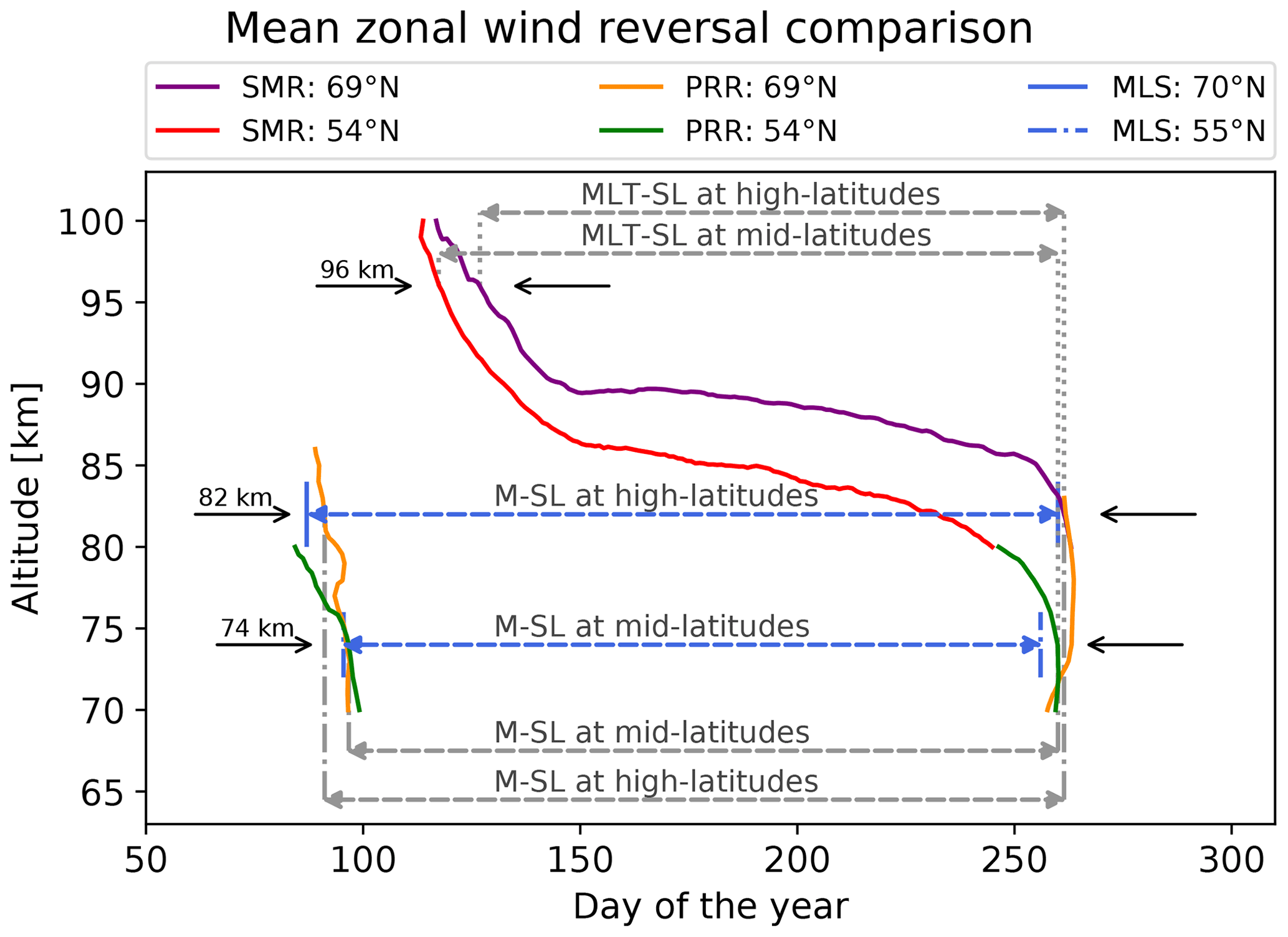
Figure 2 Mean zonal wind reversal comparison and summer length definitions (MLT-SL and M-SL) at high and middle latitudes. The mean zonal wind reversal (0 m s⁻¹) extracted from the climatologies from SMRs (purple) and PRR (orange) at 69^∘ N and SMRs (red) and PRR (green) at 54^∘ N. In addition, the specific geopotential heights with the zero zonal mean geostrophic zonal wind values from the MLS (blue) are shown at 70^∘ N (solid line) and at 55^∘ N (dash-dotted line). The black arrows indicate the altitude taken for the mean zonal wind reversal used in the individual definitions.

3.1 Mesosphere and lower-thermosphere summer length

The MLT-SL definition is established by the mean zonal wind reversal from westward to eastward at both the upper and lower altitudes. The altitudes depend primarily on the temporal evolution of the mean zonal wind reversal and in consequence on the latitude. These altitudes are chosen where the mean zonal wind reversal occurs rapidly and simultaneously for several kilometers. Considering these characteristics, at high latitudes the MLT summer beginning (SB) is chosen at 96 km height and the MLT summer end (SE) at 82 km (Fig. 2, purple line). At middle latitudes, the MLT-SB altitude is the same as at high latitudes (i.e., 96 km), but the MLT-SE was chosen at 74 km, using PRR data (see the combination of the red and green lines in Fig. 2). In both definitions, the summer length is the difference between the summer end and summer beginning.

3.2 Mesosphere summer length

The M-SL is selected at the same altitude, varying only by latitude. The summer beginning and summer ending are considered when the final mean zonal wind reversal occurs from eastward to westward and later from westward to eastward, for high latitudes at 82 km and for middle latitudes at 74 km (see Fig. 2, orange and green lines, respectively). The same altitudes are taken for the MLS (see Fig. 2 blue lines, solid lines at high latitudes and dash-dotted lines at middle latitudes). M-SL has been selected to allow a direct comparison between the MLS and radar observations and other definitions. Moreover, this definition can also be compared with models since most of them are able to reproduce the observed wind field below 90 km during April and May (e.g., Hoffmann et al., 2010; Conte et al., 2018; Pokhotelov et al., 2018).

4 Results

Here we briefly describe how the radar data have been processed and the results are obtained. We first calculate the daily mean of hourly winds for each altitude and site. Then the mean is smoothed by a 16 d running window, shifted by 1 d. In order to compress the data and to further reduce its variability and to be able to focus on the long-term changes, we implemented a principal component analysis (see details in Sect. 2). With the first two components of principal component analysis, we are able to reconstruct the mean zonal winds year by year and, considering only the altitudes of interest, we extract the day of the year (DOY) on which the reversal occurs. Following this analysis, we obtain three different time series for each latitude and definition (summer beginning, summer end, and summer length). Each time series is treated with a default standard deviation error from the size of the smoothing window plus an extra consideration for the years where the mean zonal wind reversal is particularly difficult to assess due to an unclear transition. In these cases, the sum of days during the unclear reversal period is divided by 2 and manually implemented as an error for the particular value.

Figure 3 Summer length at high latitudes: on the left is shown MLT-SL and M-SL on the right: panel (a) represents the summer beginning at 96 km (MLT-SB) and panel (e) 82 km (M-SB) for each year (abscissa) and the DOY when the mean zonal wind reversal occurs (ordinate). The summer end is measured at 82 km for both (b) MLT-SE and (f) M-SE. Panels (c) and (g) depict the summer length as the difference between summer end and summer beginning, i.e., MLT-SL and M-SL, respectively. For each time series a linear fit is shown in the same color with the standard deviation of the slope in the same color with dashed lines. The panels in the last row (d, h) show proxies of lower and extraterrestrial atmospheric forcing (see text for details).

Figure 3 presents the detected wind reversal dates at high latitudes, i.e., MLT-SL (left column, purple lines) and M-SL (right column) for the previously introduced altitude definitions. Note that for M-SL, both MLS (blue lines) and PRR (red lines) results are included. The first three panels for both definitions (Fig. 3a, b, c and e, f, g) depict the DOY (ordinate) when the mean zonal wind reversal occurs for every year (abscissa) for summer beginning, summer end, and summer length, respectively.

To explore the long-term behavior, we fit a linear function and apply the Student's t test (with null hypothesis being the slope equal to zero) to investigate whether there is a significant slope incorporating the standard deviation error propagation (e.g., Santer et al., 2000). The linear regression (solid line in the same color) is only shown for the summer beginning and summer length (first and third panels, respectively), and enclosed in dashed lines (same color) is shown the expected variability. In the case of summer end for both definitions, the linear regression is not shown since we were not able to reject the null hypothesis.

Table 1 Summary of the mean values and their standard deviations for each time series with the corresponding values of the slope from the linear fit and confidence values (cv) divided into three categories: less than 80 % without a star, greater than 90 % with one star and greater than 95 % with two stars.

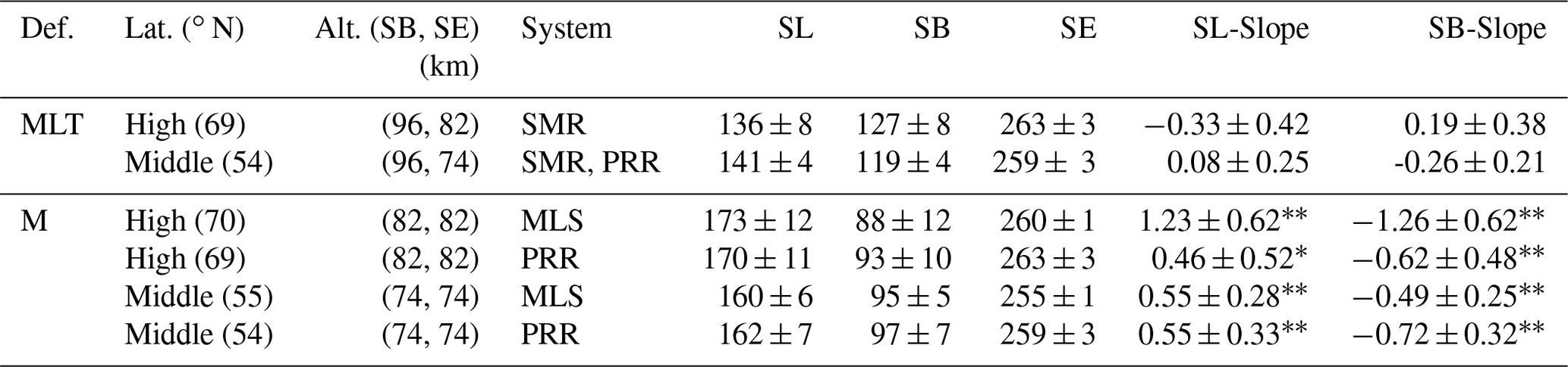
Confidence value: ${}^{\ast \ast }$cv > 95 %, ^∗cv > 90 %.

The M-SL (Fig. 3g) for the high latitudes is found to be 170±11 d long using PRR measurements (173±12 d for the MLS) with a tendency of 0.46±0.52 d yr⁻¹ (1.23±0.62 d for the MLS). Most of the variability and trend is introduced by the summer beginning (Fig. 3a) occurring at DOY 93±10 d for PRR (3 April) and DOY 88±12 d for the MLS (29 March), with a tendency to start earlier, $-\mathrm{0.62}\pm \mathrm{0.48}$ and $-\mathrm{1.26}\pm \mathrm{0.62}$ d, respectively. For the MLT-SL (Fig. 3c) we found 136±8 d but with no significant trend starting around 7 May (see Table 1 for more details).

The last row for both definitions (Fig. 3d, h) represents proxies of possible forcing in the MLT region that occurred during the corresponding previous winter (for MSSW and strong polar-night jet oscillations) or centered in the mean value for the summer beginning (March, April, and May) for Lyman α line (black line), QBO and ENSO. ENSO is represented by the Oceanic Niño Index (ONI), where the values over 1 ^∘C are considered an El Niño phase (orange) and under −1 ^∘C a La Niña (green) (see, e.g., Pedatella and Liu, 2012). The QBO is represented by the winds at 10 hPa from Singapore (scaled by 10 m s⁻¹). QBO eastward (QBOe) is shown in red, and QBO westward (QBOw) is blue. The MSSWs are represented (in purple) as follows: when a displacement of the polar vortex occurred is indicated by a “D”, and in case of a split it is indicated by the bow tide symbol. The pink “sPJO” shows the year when strong polar-night jet oscillations occurred.

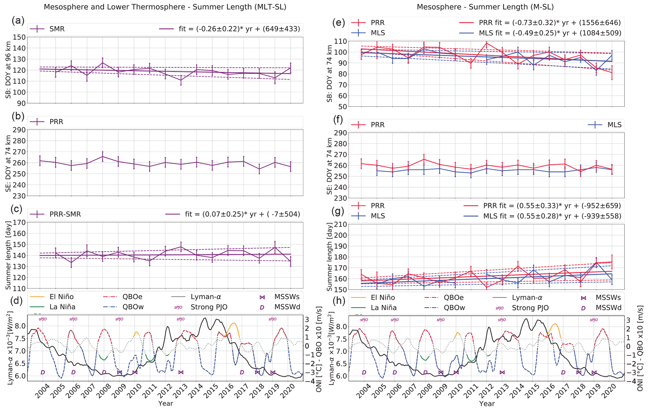
Figure 4 Summer length at middle latitudes: similar to Fig. 3, but in this case, the altitude of MLT-SE (b) is 74 km as well as for M-SB (e) and M-SE (g). At this latitude the MLT-SL is obtained from a combination of SMRs and PRR.

The middle-latitude results are shown in Fig. 4 in a similar format. The main difference is that the altitude for the summer end in both definitions is 74 km. There, the M-SL (Fig. 4g) is found to be 162±7 d long using PRR measurements (160±6 d for the MLS), with an almost identical tendency of 0.55±0.3 d yr⁻¹ for the PRR and MLS. Equivalently to the high latitudes, this mostly corresponds to the summer beginning (Fig. 4a) occurring at DOY 95±5 d for PRR and DOY 97±7 d for the MLS (between 5 and 7 April) with tendencies of $-\mathrm{0.49}\pm \mathrm{0.25}$ and $-\mathrm{0.72}\pm \mathrm{0.32}$ d, respectively. For the MLT-SL (Fig. 4c) we found 141±4 d, but again with no significant trend, starting on 29 April.

The mean values, with the standard deviations from Figs. 3 and 4, are summarized in Table 1, as well as the slopes for the summer beginning and summer length with their standard deviations. The slopes are classified from the result of the Student's t-test, as follows. The slopes with less than 80 % of confidence have no stars, more than 90 % have one star, and more than 95 % have two stars.

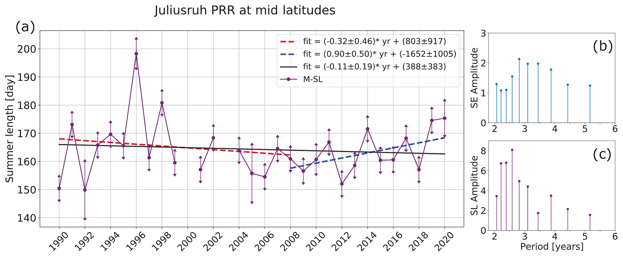
Figure 5 (a) Mesosphere summer length at middle latitudes for 31 years of measurements from Juliusruh PRR. The points show the M-SL obtained from the difference between summer end (SE) and summer beginning (SB) at 74 km. The dashed lines show the linear fit for each interval, from 1990 to 2008 in red and from 2008 to 2020 in blue. The black line denotes the linear fit for the complete time series. On the right, the summer end (b) and summer length (c) periods in years obtained by the Fourier transformation.

As mentioned previously, in the case of middle latitudes one can extend the study of the M-SL using the Juliusruh PRR to 31 years by combining zonal winds obtained at the same place but with different partial reflection radar systems and measuring techniques. Figure 5 depicts the M-SL values from this combined data set covering the period 1990–2020. In this case, we show a linear function for the entire time series in black. Due to an apparent breakpoint around 2008, we include two linear regressions according to this breakpoint, i.e., 1990–2008 in dashed red line and 2008–2020 in dashed blue line. The breakpoint was obtained by a second-degree polynomial fitted by the least square method.

5 Discussion

In this section we discuss the obtained result. Noteworthy, for both latitudes and definitions, is that the variability of the summer lengths is dominated by the summer beginning and, thus, by the winter conditions. Since our results display a latitudinal dependency, we also divided our discussion by latitude. In addition, we discuss the results of our summer definitions with respect to other definitions used in earlier studies. The long-term behavior of our results, including the 31-year analysis, is discussed separately.

5.1 High latitudes

As both definitions represent different processes from the different altitudes (in the summer beginning) and therefore times in the year, there is also a significant difference observed in the variability. The observed variability is higher in M-SB due to the proximity to the winter conditions, which is modulated by the planetary wave activity, final warmings, etc. (Lauter and Entzian, 1983; Hoffmann et al., 2002; Savenkova et al., 2012).

The MLT-SL shows peculiar values for the years 2004, 2012 and 2013, with an earlier MLT-SB. The 2013 winter-to-summer transition was reported by Fiedler et al. (2015) as an uncommon year with extreme conditions showing lower temperatures (∼6 K below the mean) and a higher concentration of water vapor at 83 km. In their study, they found strongly enhanced planetary wave activity uncommon for the time of the year (see Fiedler et al., 2015, Fig. 5).

A similar period was recently studied at the MLT Northern Hemisphere high latitudes by Hall and Tsutsumi (2020). The authors reported on temperatures at 90 km over Svalbard (78^∘ N), calculating monthly mean values and fitting trends using December as a representation of winter trends. The authors found lower temperature values in the winters 2003/2004 and 2012/2013 and reported 2012 as a change point detected by their algorithm (see Hall and Tsutsumi, 2020, Fig. 3). Even though both data sets are different (December monthly mean temperature at 78^∘ N and mean zonal wind reversal in May at 69^∘ N), these data “outliers” appear to be connected.

In the case of M-SL the years 2012 and 2016 strongly deviate from the mean behavior of the M-SL. In 2012 the satellite data show an early M-SB (DOY 74), while the radar (DOY 89) depicts a value not far from the mean (DOY 92). At high latitudes, in the Northern Hemisphere the winter is dominated by the behavior of the polar vortex and its temporal dependence on the position. Considering the satellite zonal mean geostrophic zonal winds are an average in longitude and the radar only shows the mean zonal wind at a fixed longitude, it is reasonable to find differences between these individual observations. Thus, here we can see the complexity of understanding the winter time in a localized position (radar site) compared with the average in longitude (obtained from satellite). In contrast to this example, 2016 has an earlier M-SB for both instruments (DOY 61 PRR and DOY 57 MLS) as a consequence of the event categorized as a final warming (Yamazaki and Matthias, 2019). In contrast to this categorization, Manney and Lawrence (2016) described 2016 as a major final sudden stratospheric warming.

In the time series we were not able to find a relation to Lyman α. In the case of ENSO and QBO, we also do not find a clear connection with the mean zonal wind reversal dates. A similar result is obtained analyzing the MSSW, strong polar-night jet oscillation years and the summer beginning time series. We can only find two particular clear cases where the summer beginning is affected by a final warming.

5.2 Middle latitudes

As we move far away from the polar vortex and approach the middle latitudes, the summer beginning displays less variability than at high latitudes, and there is a clear time–latitude difference in the time series (also indicated in Fig. 2). The mean zonal wind reversal occurs earlier at high latitudes and later on at middle latitudes. Towards the end of the summer, the westward wind velocity decreases and finally reverses again to the eastward direction at middle latitudes and later on at higher latitudes. Thus, the summer length difference is dependent on the latitude as a consequence of the residual mesospheric wind circulation (e.g., Andrews et al., 1987; Hoffmann et al., 2002). The mean zonal wind reversals for both latitudes exhibit a comparable profile, while the mean zonal wind reversal at high latitudes occurs at about 5 km higher altitudes (see Figs. 1 and 2). Thus, for the use of the same upper altitude (96 km), the mean zonal wind reversal occurs earlier at middle latitudes. Furthermore, small differences in the profile steepness are visible; i.e., the wind reversal does not occur simultaneously at several altitudes. However, near and especially above 100 km altitude, the meteor count rates decrease substantially, introducing larger uncertainties, which restrain us from selecting a higher altitude (e.g., Younger et al., 2009), where we exactly want to observe the mean zonal wind reversal and MLT-SB.

Looking into the unusual years seen at high latitudes, the reversal during 2012 (Fig. 4a) occurs on DOY = 116, representing an earlier start but within the variability. However, the reversal occurs on the same day at both latitudes, raising the question of what kind of event might produce a reversal of the wind on the same day at 15^∘ latitude difference. 2013 shows a deviation of 8 d apart (DOY 111) from the mean behavior in the MLT-SB but well outside of the mean standard deviation of 4 d. This difference shows again evidence of latitudinal difference and the earlier starts, which once more could be representing an unusually strong planetary wave activity for this time of the year (Fiedler et al., 2015). The M-SB (Fig. 4e) depicts a higher variability than MLT-SB, but the only year with a slight deviation from the mean behavior is 2012 with a late final warming. In addition, this late final warming and the difference between the satellite and the radar could be indicating the displaced polar vortex near the radar site.

Once more, similarly to high latitudes, the mean zonal wind reversal dates do not depict a connection to the solar activity or the other events (i.e., ENSO, QBO, strong polar-night jet oscillation or MSSW).

5.3 Comparisons with other definitions

Comparing the definitions proposed in this work with the one made by Offermann et al. (2004), we can find a big difference for the summer end. While Offermann et al. (2010) showed opposite sign slopes retrieved from a threshold in temperature in the beginning and end, we have found a variability dependence on the summer beginning. This difference is attributed to the rapid wind changes in September; meanwhile, the temperature appears to change with a weaker gradient. The summer duration obtained in their works is comparable with the values obtained for M-SL at middle latitudes, with a difference of around 10 d.

Inspired by the comparison between the summer duration in the MLT and that at ground level made by Offermann et al. (2004), we investigate the summer length through the vegetation growing season length. A recent study on the topic was performed by Hurdebise et al. (2019) with the tree Fagus sylvatica in eastern Belgium between the years 1997 and 2014, obtaining a “leafed period length” (or growing season length) of 165±7 d and a slope of −0.62 d yr⁻¹ with high significance (statistical p-value <0.05). Chen et al. (2019) studied three different species of trees (among them the Fagus sylvatica, presenting less change rate between the studied species) common in central Europe (47–55^∘ N) between 1950 and 2013. They found that since 2000 the length of the growing season has not increased, and their mean value is around 174 d. These studies show a connection between the temperatures and the leaf unfolding and folding periods at ground level for middle latitudes. The Zhou et al. (2001) extrapolated value gives us a mean of the vegetation growing season length of 160±4 d (maintaining their own standard error), comparable with M-SL at middle latitudes (160–162±7 d). In the case of Hurdebise et al. (2019) the resulting length of the vegetation growing season is 169±7 d, and for Chen et al. (2019) it is 174 with an apparent variability of around 3 d. In these cases, the M-SL is more similar to the length obtained at high latitudes (170–173±12 d), even though their studies were performed for middle latitudes.

5.4 Long-term analysis

A linear regression was implemented for all the time series and the result proven with a Student's t-test. Since in all the summer ending times series we were not able to reject the null hypothesis, we only show the significance levels for the summer beginnings and summer lengths. However, the MLT-SL definition shows no significant linear change over the years and, thus, we consider this definition to be not sensible to a possible long-term change. On the other hand, the M-SL and M-SB show linear tendencies with confidences greater than 95 % in most of the cases. The only exception is in M-SL at high latitudes (Saura PRR), where the slope shows a confidence greater than 90 % (see Table 1). In none of the time series did we apply a correction by QBO or solar activity as they were used in other works (e.g., Offermann et al., 2010; Keuer et al., 2007). In the case of QBO, the influence is not clear or seen in the mean zonal wind reversal dates, probably due to the short time series. Pursuing this concept, we extended M-SL at middle latitudes with the available data, obtaining a 31-year time series (see Fig. 5a). The summer beginning revealed periods of 2.21–2.58 years and the summer end periods of 2.82–3.87 years. Due to the low amplitude in the summer end, the summer length only reveals those found in the summer beginning (see Fig. 5b and c). These periods are associated with QBO and ENSO, 2.2–2.4 and 3.5 years, respectively (e.g., Offermann et al., 2015).

The slope of the 31-year linear regression (negative) shows an opposite direction (positive) to the shorter version (17-year time series, Fig. 4g), which made us speculate about a non-uniform trend. An inflection point is detected around 2008±2 years, and the high variability occurs mostly because of the higher uncertainties in the earlier years of the data set, where the radar experienced several changes (see Sect. 2). These uncertainties may influence the determination of the breakpoint year, and we might be in the presence of another breakpoint around 1992–1995. Moreover, the results from the spectra of the individual time series (i.e., 1990–2007 and 2008–2020) are similar to the ones in Fig. 5b and c. Particularly in the 2008–2020 time series, we identify periods around 2.25–2.57 years for the summer end, while in the summer beginning 3-year and 4.5-year periodicities are identified. Nevertheless, the 4.5-year amplitude is not as relevant as the 3-year one, but it could be associated with a quasi-quadrennial oscillation (French et al., 2020).

Evidence of breakpoints in the long-term studies has been reported by several authors. Lauter and Entzian (1983) speculated a period of 10–20 years after finding a breakpoint in 1980. The same year was identified by Offermann et al. (2004, 2005), and Offermann et al. (2006) reported an additional one in 2001/2002. Studying the amplitudes of the mean zonal winds during different seasons, Liu et al. (2010) and Jacobi et al. (2015) described a breakpoint in the summer months around 1995–2000 in Collm observations. Later on, Hall and Tsutsumi (2020) detected a breakpoint in 2012±1 year. Portnyagin et al. (2006) found a breakpoint in 1980 and adjusted two different linear functions and parabolas, concluding that at middle latitudes, the MLT winds have non-uniform trends. With our initial time series (2004–2020), we cannot see a clear indication of a breakpoint. Nevertheless, it is detected within 31 years of measurements. Considering the numerous studies and our findings, we can only assume that a more robust trend analysis might require a longer time series.

6 Summary and conclusions

Smoothed mean zonal winds between 2004/2005 and 2020 from different radars located at high and middle latitudes (Andenes SMR–Tromsø SMR, Saura PRR, Juliusruh SMR–Collm SMR and Juliusruh PRR), as well as MLS measurements, are used to study two different summer length definitions (see Sect. 3). The MLT-SL definition is taken when the last wind reversal occurred from westward to eastward at 96 km (MLT-SB) and 82 km at high latitudes (74 km for middle latitudes) as MLT-SE. On the other hand, the M-SL definition is taken at the same altitude (M-SB and M-SE) but depending on the latitude (82 km at high latitudes and 74 km at middle latitudes), when the mean zonal wind reverses from eastward to westward (M-SB) and, again, from westward to eastward (M-SE).

With the obtained time series, we analyzed the summer length and studied the variability and the linear tendency. We looked into the dates and the different events occurring in the upper and lower atmosphere to understand the events modifying the summer length. Furthermore, we compared the summer length to the growing season length. The results are summarized as follows.

• The summer length is determined by the mean zonal wind reversal, which depends on the actual latitude and altitude. High latitudes showed more variability than middle latitudes for both definitions. The summer beginning presents most of the variability that is transferred to the summer length. The summer end occurs for all latitudes in the same week before the autumn equinox and presents no significant linear trend.

• MLT-SL definition: the summer starts around 7 May at high latitudes (SL = 136 d) and around 29 April at middle latitudes (SL = 141 d), showing a shorter summer length at high latitudes. This definition presents no significant trends, and the events studied (MSSW, strong polar-night jet oscillations, ENSO, QBO and Lyman α) do not seem to affect the duration of the summer. Nevertheless, we have found strong evidence of abnormal behavior in the years 2004, 2012 and 2013, also observed by Hall and Tsutsumi (2020). Particularly the year 2013 has been reported by Fiedler et al. (2015) as presenting high planetary wave activity later than the usual time, producing an earlier mean zonal wind reversal.

• M-SL definition: this is more variable than the MLT-SL due to the higher variability in the summer beginning, which is more prone to the winter conditions. The summer starts between the end of March and the beginning of April for high latitudes and 1 week later at middle latitudes (see Table 1). In this case, linear trends were found for summer beginning and summer length with 90 % or more confidence. The years 2012 and 2016 displayed extreme values. However, in the latter, the earlier summer beginning was a consequence of a final warming (Yamazaki and Matthias, 2019).

• At middle latitudes, the length of the growing season at ground level is similar or has around 10 d difference (depending on the author) to the M-SL.

• After analyzing the time series and trying to relate it to other events (solar activity, QBO, ENSO, strong polar-night jet oscillations, and MSSW), we were not able to find a direct influence on the summer length or summer beginning. Only for the M-SL did we find 1 year (with a strong MSSW and 2016 final warming) being directly affected. The 17-year time series are short for studying the period related to QBO or ENSO. On the other hand, with the 31-year time series (see Fig. 5), we detected periodicities of around 2.21–2.58 and 2.82–3.87 years that we could attribute to QBO and ENSO, respectively (e.g., Offermann et al., 2015).