A multi-instrumental and modeling analysis of the ionospheric responses to the solar eclipse on 14 December 2020 over the Brazilian region

This work presents an analysis of the ionospheric responses to the solar eclipse that occurred on 14 December 2020 over the Brazilian sector. This event partially covers the south of Brazil, providing an excellent opportunity to study the modifications in the peculiarities that occur in this sector, as the equatorial ionization anomaly (EIA). Therefore, we used the Digisonde data available in this period for two sites: Campo Grande (CG; 20.47^∘ S, 54.60^∘ W; dip ∼23^∘ S) and Cachoeira Paulista (CXP; 22.70^∘ S, 45.01^∘ W; dip ∼35^∘ S), assessing the E and F regions and E_s layer behaviors. Additionally, a numerical model (MIRE, Portuguese acronym for E Region Ionospheric Model) is used to analyze the E layer dynamics modification around these times. The results show the F1 region disappearance and an apparent electronic density reduction in the E region during the solar eclipse. We also analyzed the total electron content (TEC) maps from the Global Navigation Satellite System (GNSS) that indicate a weakness in the EIA. On the other hand, we observe the rise of the E_s layer electron density, which is related to the gravity waves strengthened during solar eclipse events. Finally, our results lead to a better understanding of the restructuring mechanisms in the ionosphere at low latitudes during the solar eclipse events, even though they only partially reached the studied regions.

1 Introduction

Events such as a solar eclipse, where the moon passes between the Sun and the Earth, can cause modifications in the ionosphere. The solar radiation is attenuated, and, consequently, the UV solar flux decreases, affecting all the ionospheric layers (Fargues et al., 2001; Chandra et al., 2007; Vogrincic et al., 2020). Thus, it is possible to observe influences in total electron content (TEC) (Cherniak and Zakharenkova, 2018a) in the equatorial ionospheric anomaly (EIA) (C. H. Chen et al., 2019; Jonah et al., 2020), a decrease in the E and F region densities (Chandra et al., 2007), and changes in all types of sporadic E (E_s) layers (Adeniyi et al., 2007; Pezzopane et al., 2015).

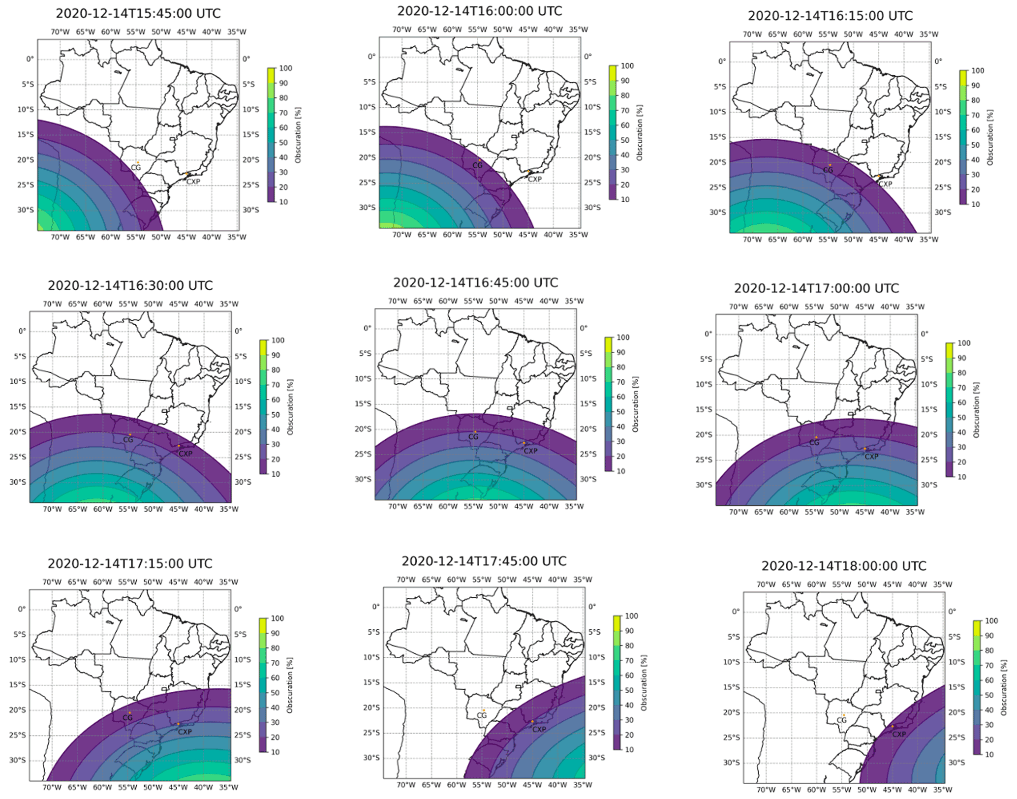
Figure 1 Eclipse obscuration mask at 250 km height between 15:45 and 18:00 UT for every 15 min on 14 December 2020. The contour colors are obscuration varying from 10 % (purple) to 100 % (yellow). CG and CXP are marked in these maps, referring to the Digisonde stations.

Many studies about the ionosphere response in partial or total solar eclipse were performed in the last years. Sridharan et al. (2002) analyzed the ionosphere electrodynamics during the solar eclipse on 11 August 1999, over the equatorial station in Trivandrum, India (8.5^∘ N, 77^∘ E; dip 0.5^∘ N). Their results showed some characteristics in the ionograms as intense blanketing E_s layer (E${}_{{\mathrm{s}}_{\mathrm{b}}}$) occurrence and an increase in the F region virtual height (h^′F) after the solar eclipse, emerging as the spread-F structures. The authors concluded that the solar eclipse could lead to favorable conditions for irregularity development. Chernogor et al. (2019) recently analyzed the solar eclipse effects in the mid-latitude daytime ionospheric plasma. The eclipse event occurred along with the magnetic storm recovery phase on 20 March 2015. However, the authors concluded that the increases in the F region peak height (hmF2) during the maximum solar occultation and the decrease in the electron density around 190–210 km are consequences of the solar eclipse.

Huba and Drop (2017) used the Naval Research Laboratory (NRL) model Sami3 to predict the total solar eclipse impact that occurred on 21 August 2017 on the ionosphere and plasmasphere. The authors observed the 35 % reduction of the TEC during the eclipse hours. Cherniak and Zakharenkova (2018b) and C. H. Chen et al. (2019) studied the same event in the American sector. Both studies analyzed the TEC maps during the solar eclipse. They found a TEC decrease of ∼30 %–40 % along the totality path within an area of 75 % obscuration. In fact, their work showed that the vertical electronic density latitudinal variations presented enhancements or reductions of EIA crests depending on the latitude.

Regarding the E_s layer behavior, Chen et al. (2010a, b) and Tiwari et al. (2019) showed a considerable enhancement in their electronic density, meaning that an intensification of the E_s layer occurred during the total solar eclipse on 22 July 2009. Pezzopane et al. (2015) analyzed the E_s layer using the ionosondes located at mid-latitude stations of Italy during the solar eclipse that occurred on 20 March 2015. They found that the solar eclipse affects the temporal persistence of the E_s layer. In all these studies, the E_s layer changes were attributed to gravity wave occurrences caused by thermal gradients related to the solar eclipse event. On the other hand, G. Chen et al. (2019) investigated the E_s layer response during the solar eclipse in the American continent on 21 August 2017. They found an intensity reduction of these layers during this event, which they associated with the photoionization decrease.

Martínez-Ledesma et al. (2020) predicted the F region behavior during the total solar eclipse on 14 December 2020. They used the Sheffield University Plasmasphere Ionosphere Model (SUPIM-INPE) (Bailey et al., 1993; Souza et al., 2010) to evaluate the TEC modifications at low latitudes. The predictions expected a TEC decrease of up to 22 % in regions along the path of totality. Also, the simulations showed a minor TEC reduction around the magnetic equator locations that even so affected the fountain effect and, consequently, the EIA crests.

In this work, we perform a multi-instrumental and modeling analysis of the ionospheric response over low latitudes in the Brazilian regions predicted by Martínez-Ledesma et al. (2020) for the solar eclipse event on 14 December 2020. We used the Digisonde data to observe the modifications in the E and F regions and the E_s layers over two sites: Campo Grande (CG; 20.47^∘ S, 54.6^∘ W; dip ∼23^∘ S) and Cachoeira Paulista (CXP; 22.70^∘ S, 45.01^∘ W; dip ∼35^∘ S). Also, a numerical model (MIRE, Portuguese acronym for E Region Ionospheric Model) is used to analyze the E layer chemistry. The TEC maps derived from the Global Navigation Satellite System (GNSS) are used to observe changes in the EIA. Finally, the results showed that solar eclipses can cause significant ionosphere modifications even though they only partially reach the Brazilian low-latitude regions.

2 Methodology

In the following, we briefly describe each set of data used in this study: Digisonde data, GNSS TEC variation, and MIRE model.

2.1 Digisonde data

In this work, we used ionospheric parameters of the vertical electron density profiles obtained from Digisonde, called ionograms. This equipment is a high-frequency (HF) radar that transmits radio waves continuously into the ionosphere ranging from 1 to 30 MHz (Reinisch et al., 2009). We used the Digisonde data from CXP and CG over the Brazilian sector provided by the Brazilian Studies and Monitoring of Space Weather (EMBRACE) program (available at http://www2.inpe.br/climaespacial/portal/en/, last access: 2 October 2021).

We evaluated the F region behavior using height parameters, such as the virtual height (h^′F) and peak height (hmF2), which is important to investigate the changes in this region. Also, we analyzed the frequency parameters of the F and E regions and E_s layer (foF2, foE, and fbE_s, respectively), which are related to the electronic density at the layer peak. The fbE_s is the frequency at which reflection from a layer at superior heights starts to be visible in ionograms. The time resolution is 10 min from the ionograms in stations considered here.

2.2 TEC analysis

The GNSS receiver data were used to obtain the total number of electrons (TEC) in a given ionospheric path. TEC is a measurement of the electrons in a column of unitary cross-sectional area between the satellite and the receiver. Due to the high number of stations over the Brazilian sector, it is possible to construct the two-dimensional maps of the absolute vertical TEC values ranging from 50 to ∼500 km of spatial resolution in latitude and longitude, every 10 min (Otsuka et al., 2002; Takahashi et al., 2016). This current work analyzes the EIA during the eclipse occurrence using these maps, available online on the EMBRACE website.

2.3 MIRE model

We have used a theoretical model, called MIRE, which provides the E region and E_s layer electron densities as follows (Carrasco et al., 2007; Resende et al., 2017a, b, 2020, 2021):

$$\begin{array}{}\text{(1)}& ne=\left[{\mathrm{O}}_{\mathrm{2}}^{+}\right]+\left[{\mathrm{NO}}^{+}\right]+\left[{\mathrm{O}}^{+}\right]+\left[{\mathrm{N}}_{\mathrm{2}}^{+}\right]+\left[{\mathrm{Fe}}^{+}\right]+\left[{\mathrm{Mg}}^{+}\right].\end{array}$$

This model solves a set of partial differential equations of the continuity and momentum between 00:00 and 24:00 UT in the height range from 86 to 120 km for the main molecular or atomic ions in the E region (NO⁺, ${\mathrm{O}}_{\mathrm{2}}^{+}$, ${\mathrm{N}}_{\mathrm{2}}^{+}$, O⁺), as well as metallic ions (Fe⁺, Mg⁺).

The MIRE continuity equation of each constituent N_i,

$$\begin{array}{}\text{(2)}& {\displaystyle \frac{\partial \left[N_i\right]}{\partial t}}=P-L-{\displaystyle \frac{\partial V_{iz}\left[N_i\right]}{\partial z}},\end{array}$$

is used to calculate the ion density by taking into account the production (P), loss (L), and transport $\left(\frac{\partial V_{iz}\left[N_i\right]}{\partial z}\right)$. The transport term depends on the wind and electric field parameters (Resende et al., 2020). This analysis only considers the E region chemistry, thus neglecting the transport terms and metallic ions. More details about the MIRE model can be found in Carrasco et al. (2007) and Resende et al. (2017a).

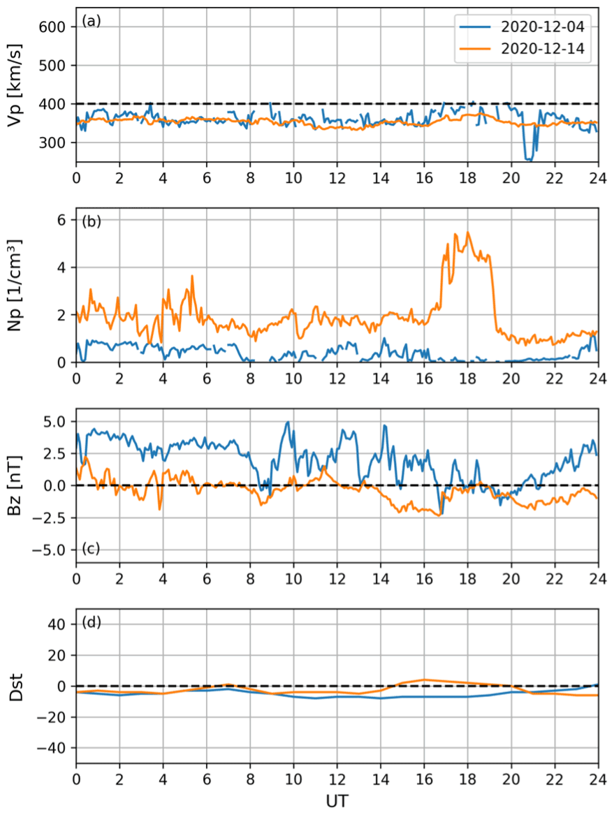
Figure 2 (a) The solar wind velocity V_p, (b) the number density of protons N_p, (c) the interplanetary magnetic field component B_z, and (d) the Dst index on 14 December 2020 (orange line) and on 4 December 2020 (blue line).

2.4 Solar eclipse characteristics

We divided this study into two ionospheric responses of the solar eclipse that occurred on 14 December 2020: (1) the ionospheric changes in the F region, and consequently EIA behavior, and (2) the E region and E_s layer behavior during the solar eclipse hours. Figure 1 shows the solar eclipse evolution between 15:45 and 18:00 UT for every 15 min at 250 km height. The colors mean the obscuration varying from 10 % (purple) to 100 % (yellow). Notice that only two Digisonde stations (CXP and CG) had a solar eclipse obscuration over the Brazilian sector with available data. In CXP, the solar eclipse influence starts about 16:15 until 18:00 UT, while in CG it was between around 16:00 and 17:15 UT. Therefore, we analyzed these regions since the solar eclipse provides a great opportunity to study the responses of the ionospheric regions to the rapid solar radiation variation.

3 Results and discussions

3.1 Space weather conditions during the eclipse 2020 versus quiet period

The interplanetary medium parameters are measured from the Proton and Alpha Monitor (SWEPAM) and Magnetic Field Experiment (MAG) instruments aboard the Advanced Composition Explorer (ACE) spacecraft (Stone et al., 1998). Figure 2 shows the solar wind speed, V_p (a), proton density, N_p (b), and B_z component of the Interplanetary Magnetic Field (IMF) (c) measured at the L1 Lagrangian point. Also, we show the Dst index in panel (d). The data for a solar eclipse that occurred on 14 December 2020 are shown with the orange line, and we used a reference period on 4 December 2020 that is shown with the blue line.

The V_p observed in the eclipse day and the quiet period is concentrated below 400 km s⁻¹, which is considerably slow wind (Tsurutani et al., 2011; Isaacs et al., 2015). The proton density fluctuates around 2 particles cm⁻³ during almost the entire eclipse day, except in a short period between 16:48 and 19:12 UT, reaching ∼5 particles cm⁻³. This short period can be associated with the solar sector boundary crossing (figure not shown here). However, these values are still considered low. Also, the B_z component fluctuates around zero during almost the entire eclipse day, reaching the maximum negative value of $\sim -\mathrm{2.5}$ nT during a short time and presenting few positive incursions (maximum of ∼2 nT). To confirm that the event occurred on a geomagnetically quiet day, we show the Dst index in Fig. 2d. Although this parameter showed a minor enhancement during the solar eclipse event starting at 14:00 UT, the values remained very low, oscillating around zero. Finally, all the interplanetary parameters showed that this day is not geomagnetically disturbed in terms of the ionosphere influence. Therefore, this event is an excellent opportunity to analyze the ionospheric influences during a solar eclipse occurrence.

3.2 Responses of the F region heights during the hours of the solar eclipse event

In Fig. 3, we investigate the minimum F layer virtual height h^′F (top) and F layer peak height hmF2 (bottom) to both analyzed regions in panels (a) CG and (b) CXP between 14:00 and 19:00 UT. The blue lines are the height parameters for the quietest day of the month (4 December 2020), whereas the red lines refer to the solar eclipse day on 14 December 2020. The grey line represents the solar eclipse obscuration for each region. At CG, the maximum obscuration occurred at 16:45 UT, reaching 20 %. On the other hand, the maximum obscuration occurred at 17:15 UT in CXP, with the most substantial value of 29 %. Unfortunately, we do not have data over Santa Maria station (29.7^∘ S, 53.8^∘ W; dip ∼37^∘ S) during the solar eclipse hour occurrences, where the maximum obscuration reached 53 %.

In both regions, we observe a strong fluctuation with high values of the h^′F before the solar eclipse onset. This behavior happens because a C4.0 class solar flare occurred between 14:09:00 and 14:56:00 UT, causing a radio blackout of the E and E_s layer regions and partially the F region (Nogueira et al., 2015). The h^′F has low values concerning the quiet reference value after 16:15 and 17:00 UT for CG and CXP, respectively. At the same hours, a constant decrease was observed in the hmF2 parameter for these regions.

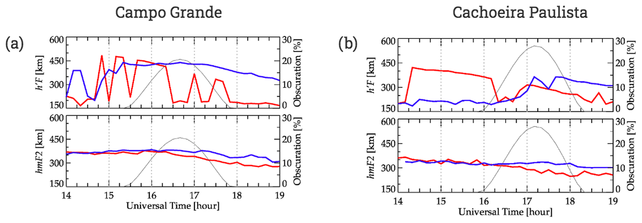
Figure 3 Virtual height h^′F (top) and F layer peak height hmF2 (bottom) in (a) CG and (b) CXP between 14:00 and 19:00 UT. These parameters are presented by the blue line for the quietest day of the month (4 December 2020), and the red line refers to the solar eclipse on 14 December 2020. The grey line represents the solar eclipse obscuration for each region in percent.

Figure 4 Ionograms collected at CG at 15:00, 17:30, and 17:50 UT, showing the F1 layer disappearance during the eclipse hours on 14 December 2020.

To better observe this scenario, we show the ionograms for both regions. Figure 4 refers to CG on 14 December 2020 for 15:00, 17:30, and 17:50 UT. Notice that in hours before the solar eclipse, the F1 region is present as the red arrow indicates. However, we observe that the F1 region has completely disappeared at 17:30 UT, returning at 17:50 UT. Here, we believe that the F1 region can suffer from the lost ionization, as discussed in Fargues et al. (2001). In fact, as the peak obscuration for the CG station occurred around 16:20 UT, the absence of the F1 region can be associated with the recombination processes during the solar eclipse. The same behavior seems to occur in CXP, as is shown in Fig. 5. In this case, we observe the F1 layer at 16:50 UT. Around 17:10 UT, this layer disappears completely. However, a strong E_s layer of type c (E${}_{{\mathrm{s}}_{\mathrm{c}}}$) caused by tidal winds (Resende et al., 2017a) appears also and can block the F region. This absence of the F1 region lasted until 18:10 UT when this layer occurred again (as seen in the ionogram at 18:20 UT). Thus, in both regions, the F1 absence lasts around 1 h, and we consider that it is due to the solar eclipse event and the E_s layer presence, which can block the F region. All these characteristics make the height profile of these regions decrease significantly, as we saw in the h^′F and hmF2 parameters in Fig. 3.

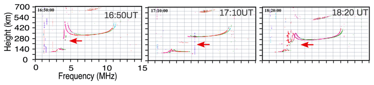
Figure 5 Ionograms collected at CXP at 16:50, 17:10, and 18:20 UT, showing the F1 layer disappearance during the eclipse hours on 14 December 2020.

Chandra et al. (2007) studied the ionospheric effects of the total solar eclipse of 11 August 1999 over the Ahmedabad region (23^∘ N, 73^∘ E). The authors did not find any decrease in the critical frequency of the F1 layer. However, Minnis (1955) analyzed the E and F1 layers during the solar eclipse of 25 February 1952. The author rewrote Chapman's equation by considering the fraction of the ionizing radiation lost during the unobscured times. The theoretical results showed significant weakness in the F1 layer due to the loss of electrons caused by an effective recombination process. More recently, Adeniyi et al. (2007) showed the solar eclipse effect on the ionosphere over an equatorial station (8.53^∘ N, 4.57^∘ E; dip 4.1^∘ S) in the African region. This event was on 29 March 2006, and the maximum obscuration was 99 % in this station. One of their results was the evident absence of the F1 regions in ionograms over the station analyzed. An explanation was that the electron density in the layers became so thin during the solar eclipse events that the ionosonde could not detect it. However, unlike our result, the E region also disappears in Adeniyi et al. (2007). In Figs. 4 and 5, the E and E_s layers are evident, leading to uncertainties about the solar eclipse effect in the ionosphere on 14 December 2020. We believe here that the electron density decreases due to the recombination factor during the solar eclipse. The E${}_{{\mathrm{s}}_{\mathrm{b}}}$ layer simultaneous appearance resulted in a significant weakening of this layer, making detection by the Digisonde difficult.

We do not observe significant differences in the F₂ layer densities in the ionograms data from these stations. Figure 6 shows the foF2 parameter for CG (a) and CXP (b) during the reference day (blue line, 4 December 2020) and during the solar eclipse event (red line, 14 December 2020). The grey line represents the solar eclipse obscuration for each region. Notice that over CG, the F region electron density (related to the foF2) was smaller than the reference day since the previous hours of the solar eclipse event. Over CXP, the foF2 values are practically the same on the 2 d analyzed. We credit this behavior to the low solar eclipse obscuration (20 %–30 %) over the ionospheric stations. The loss processes were insufficient to weaken the electron density at the F region, as seen in other events (Adeniyi et al., 2007).

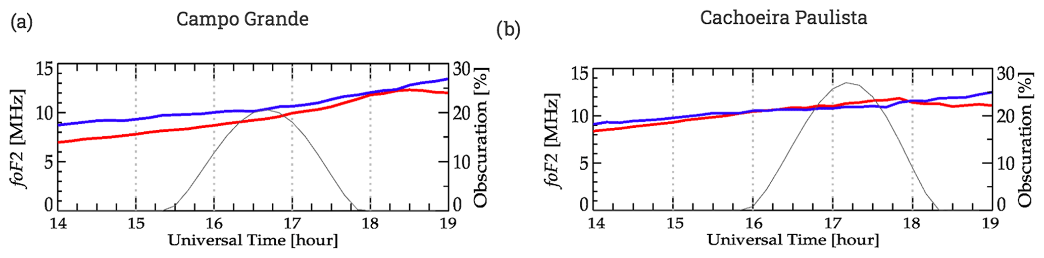
Figure 6 F region frequency (foF2) in (a) CG and (b) CXP between 14:00 and 19:00 UT. These parameters are presented by the blue line for the quietest day of the month (4 December 2020), and the red line to the solar eclipse on 14 December 2020. The grey line represents the solar eclipse obscuration for each region in percent.

The short ionization interruption could affect the EIA over the South American sector, as shown in Fig. 7. This figure shows the TEC behavior through the maps (Takahashi et al., 2016), in which we have two high-density areas between 20–30^∘ S and 40–60^∘ W that characterizes the EIA. The red line refers to the magnetic equator, the circles (Fig. 7c) refer to the eclipse area at 17:00 UT, and the color scale in Fig. 7a and b indicate the TEC intensity from 0 to 50 TECU (1 TECU =10¹⁶ electrons m⁻²). The EIA results from the equatorial plasma downward flows along magnetic field lines because of the diffusion and gravity. Therefore, two plasma crests are seen over the off-equatorial region, in the Northern Hemisphere and Southern Hemisphere (Nogueira et al., 2011). This behavior is evident in Fig. 7a, when it is possible to observe the EIA peak around ±15^∘ in TEC maps at 17:00 UT, being stronger in the southern regions. Notice that, on 14 December 2020 (Fig. 7b), we observed a clear weakening of the EIA crests compared with the typical behavior of the ionosphere plasma (Fig. 7a).

To better observe this difference, Fig. 7c shows the relative difference (RD) parameter over the TEC maps computed by

$$\begin{array}{}\text{(3)}& \mathrm{RD}\left(\mathit{\%}\right)=\left(({\mathrm{TEC}}_{\mathrm{SE}}-{\mathrm{TEC}}_{\mathrm{Ref}})/{\mathrm{TEC}}_{\mathrm{Ref}}\right)\times \mathrm{100}.\end{array}$$

The RD is calculated through the TEC maps for the solar eclipse day (TEC_SE) concerning the typical day (TEC_Ref). This result shows that the TEC is between 30 % and 50 % smaller during the eclipse occurrence over the Brazilian sector.

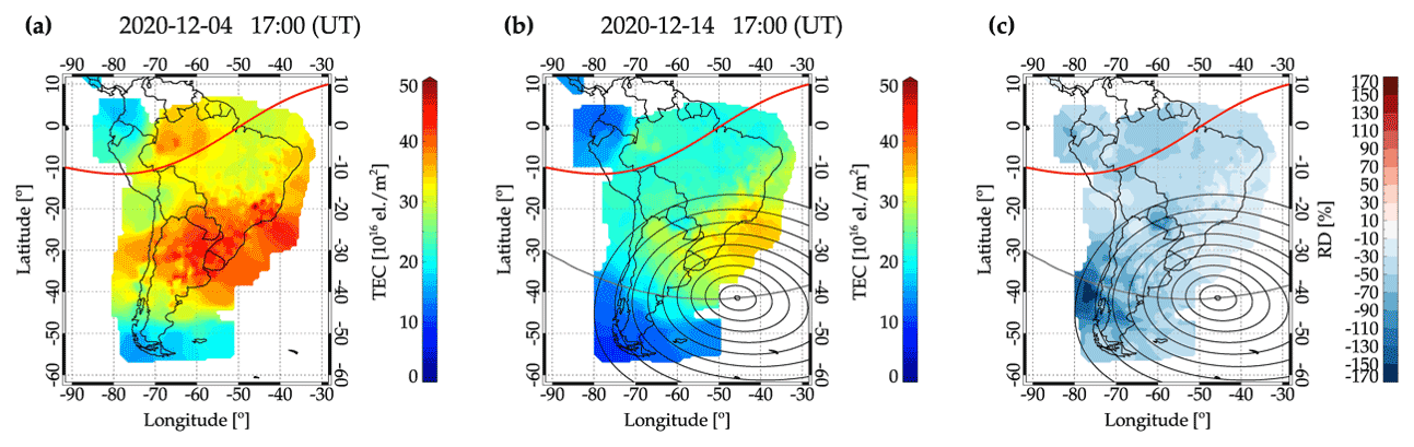
Figure 7 Longitude versus latitude distribution of the TEC map over South America (a) during the reference period (4 December 2020, at 17:00 UT), (b) during the solar eclipse event (14 December 2020, at 17:00 UT), and (c) the RD parameter. The red line refers to the magnetic equator, the circular lines refer to the eclipse area, and the color scale indicates the TEC intensity.

Vyas and Sunda (2012) analyzed the TEC changes during an annular solar eclipse over the Indian sector on 15 January 2010. They showed a TEC reduction in the EIA localization that was named as inhibited EIA region. They attributed this behavior to the combined effects of the solar eclipse, which induce attenuation of extreme ultraviolet (EUV) solar irradiation and the inhibited equatorial electrodynamics, affecting the EIA. The negative deviation was 20 %–40 % in the inhibited EIA region. C. H. Chen et al. (2019) modeled the EIA dynamic variations during a solar eclipse that occurred on 21 August 2017, around North America and South America. They also obtained the TEC difference, and their results showed a significant reduction around EIA regions at solar eclipse times. Huang et al. (2020) studied the ionospheric responses at low latitudes in a solar eclipse on 21 June 2020. The authors also found that the EIA decreases significantly in the solar eclipse hours. In summary, Table 1 presents some recent studies that observed the EIA decrease during the solar eclipse events. Hence, we show the work reference, the solar eclipse date, and the percentage of the EIA decrease concerning the typical periods.

Table 1 Some studies that observed the EIA decrease during the solar eclipse events, as well as the percentage of the EIA layer decrease.

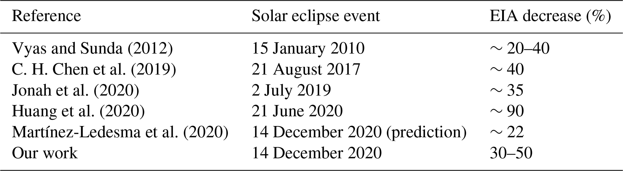
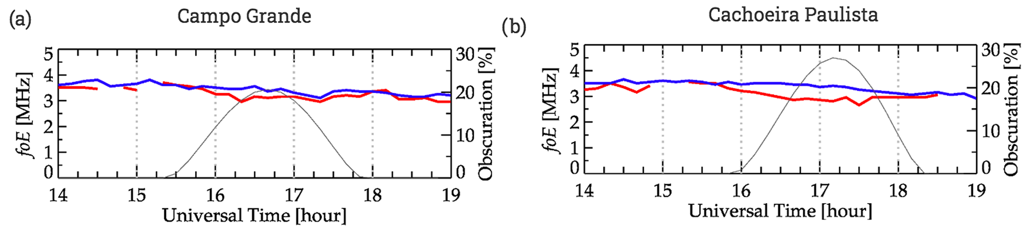
Figure 8 E region critical frequency (foE) in (a) CG and (b) CXP between 14:00 and 19:00 UT. The parameters are presented by the blue line for the quietest day of the month (4 December 2020), and the red line refers to the solar eclipse on 14 December 2020. The grey line represents the solar eclipse obscuration for each region in percent.

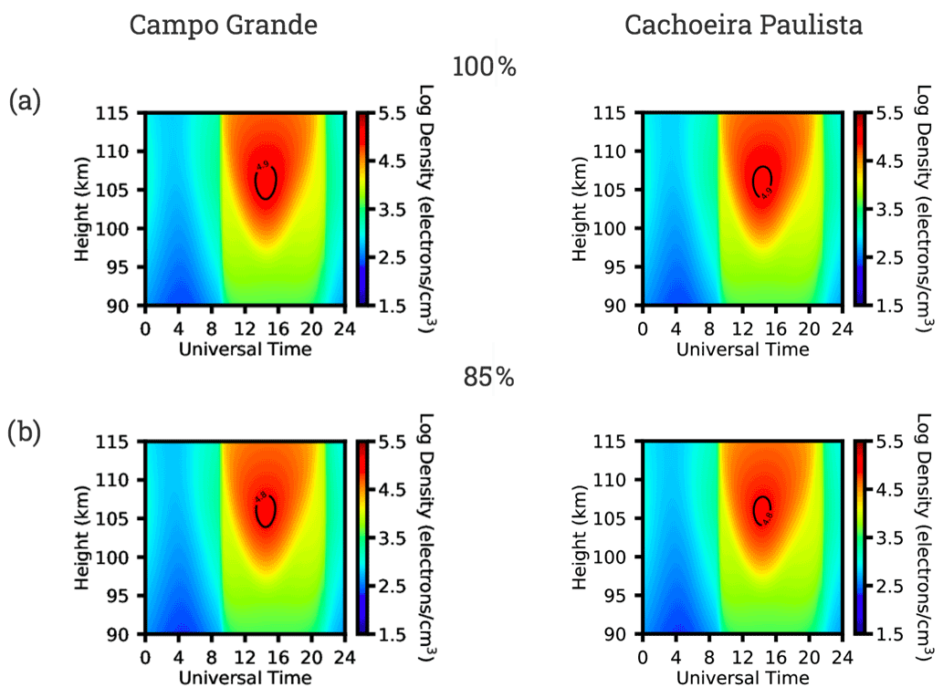
Figure 9 E region electron density simulated by MIRE considering the ionization for (a) 100 % and (b) 85 % on 14 December 2020, in Campo Grande (left panel) and Cachoeira Paulista (right panel).

All the studies cited before concluded that the ionization loss caused variation in the dynamic processes during the obscuration times, affecting the EIA behavior. The main hypothesis is that if the solar eclipse goes through the equatorial regions, the fountain effect will change, and consequently, less plasma density reaches the low latitudes. As predicted by Martínez-Ledesma et al. (2020), in our work, we believed that the minor TEC reduction around the magnetic equator locations was enough to cause a plasma density decrease in both EIA crests. Another hypothesis here is that the partial absence of the radiation over the Peruvian equatorial sector changes the conductivity in this locality and, maybe, reaches the entire equatorial area. Thus, we reduce the equatorial density, and, consequently, the fountain effect can be affected. Therefore, although this solar eclipse event almost did not reach the equatorial regions, we suppose it was enough to influence the fountain effect. Also, Huang et al. (2020) mentioned that during the eclipse events the transequatorial northward or southward neutral wind can weaken, causing a reduction of the EIA crests.

Le et al. (2009) showed an analysis of the ionosphere in the conjugate hemisphere during the solar eclipse on 3 October 2005. Their main result is a decrease in the electron temperature in both conjugate points, which is associated with a reduction in the photoelectrons traveling along the magnetic field lines from the eclipse region to the conjugate region. Thus, the authors proposed that solar eclipse events can cause a disturbance in the ionospheric regions in the conjugate hemisphere. In such an analysis, the TEC decreases around 32 % in the 300 km. Recently, Zhang et al. (2021) analyzed the TEC perturbations in the south/north EIA crests of the solar eclipse on 21 August 2017. They found that in the southern crest of the anomaly the TEC reduced significantly, while in the northern crest it stayed almost undisturbed. They mentioned that there is a northward motion tendency for plasma within the flux tubes that can inhibit the typical diffusion of the equatorial fountain effect.

We already analyzed the TEC around the days of the solar eclipse (13 and 15 December 2021). Here, we found the same behavior for the southern crest of the EIA, characterized by a decrease of around 30 %. For the northern EIA crest on 13 December we also observed a reduction in the TEC, and on 15 December, we did not see any significant modification (not shown here). Thus, this work establishes that it is possible that the plasma movement on the flux tube modified the equatorial fountain effect. However, to validate all these hypotheses, it is necessary to consider other equipment, which will be carried out in future work.

3.3 Responses of the E region and E_s layers during the hours of the solar eclipse event

The E region is dominated by the production and loss process in the ionosphere. Therefore, it is expected that the electron density of this layer suffers an influence during eclipses. Figure 8 shows the variation of the E region critical frequency parameter (foE) in CG and (b) CXP between 14:00 and 19:00 UT. The blue lines refer to the quietest day of the month (4 December 2020), and the red lines refer to the solar eclipse day on 14 December 2020. The grey line represents the solar eclipse obscuration for each region. We note that the ionization starts to decrease around 15:40 and 15:50 UT for CG and CXP, respectively. Moreover, the values remain low until 18:00 UT with respect to the quiet reference day.

We observe a decrease of around 15 % in the ionization in the E region during the solar eclipse obscuration (decrease from 4 to ∼3.3 MHz). Chernogor et al. (2019) analyzed the solar eclipse effects on 20 March 2015, on the mid-latitude daytime ionospheric plasma using observations from Kharkiv incoherent scatter radar (49.60^∘ N, 36.30^∘ E). They show that in heights less than 210 km, it is common to see a decrease in the electron density, mainly in the maximum phase of the solar eclipse. They found that the electron density reduced by 18.5 % in this event. Also, they believe that the explanation is related to the E region chemistry since the loss for recombination in these heights is quadratic. Thus, as the ionization radiation from the Sun has been removed in this region, the loss processes become effective quickly, and the E region density is affected directly. Nonetheless, Rishbeth (1968) had already reported that during partial or total eclipse events, the recombination process is not enough for the electron density to decay drastically. In fact, the authors mentioned that the duration time of the eclipse is not sufficient to affect the E region chemistry, making it disappear or diminish substantially. This fact can explain the reason for the E region electron density decrease of 15 % in our data.

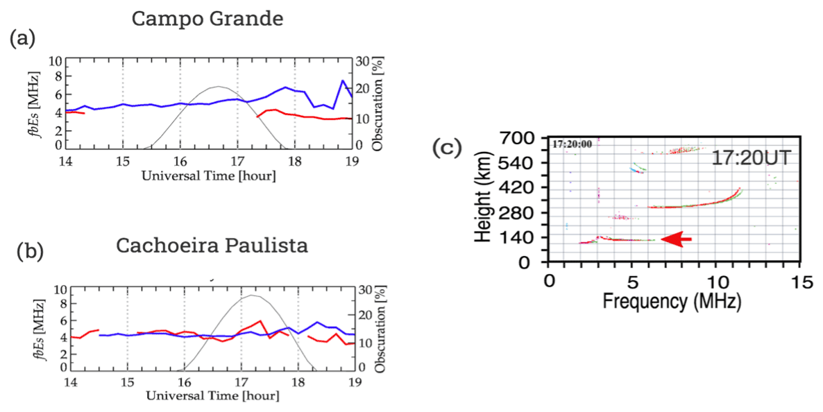
Figure 10 The blanketing frequency of the E_s layer (fbE_s) in (a) Campo Grande and (b) Cachoeira Paulista between 14:00 and 19:00 UT, and (c) the ionogram for Cachoeira Paulista at 17:20 UT. These parameters are presented by the blue line for the quietest day of the month (4 December 2020), and the red line refers to the solar eclipse on 14 December 2020. The grey line represents the solar eclipse obscuration for each region.

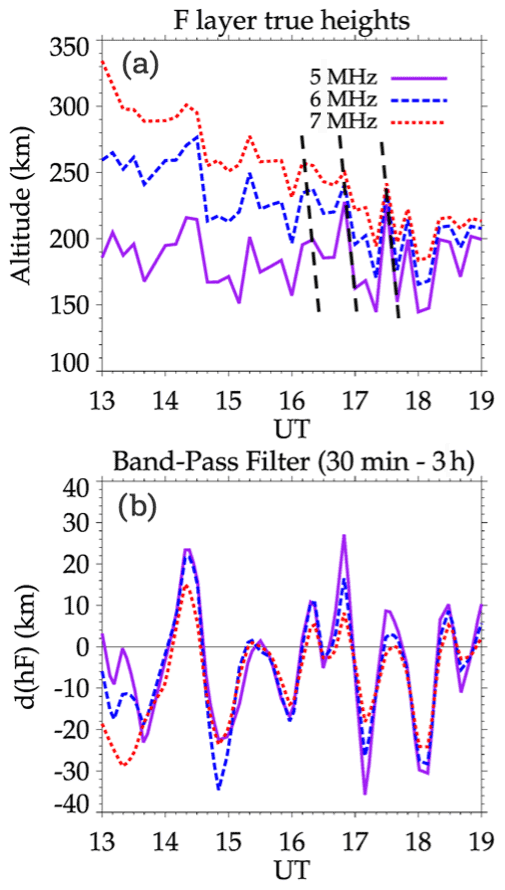
Figure 11 Temporal variations in the fixed-frequency (5, 6, and 7 MHz) true heights, hF (a), and deviation of hF (band-pass filtered (30 min–3 h)) (b) in CXP on 14 December 2020.

Figure 9 shows the E region electron density simulated by MIRE in height–time–intensity (HTI) maps over CG (left panel) and CXP (right panel). The profile background shows the regular E region, which is described by the significant electron density values in the daytime and low values during the nighttime. The metallic ions and transport terms in Eqs. (1) and (2) were negligible since they are not important to analyze the E region. We have the E region profile considering the usual conditions in panel (a) and in panel (b) we reduced the E region ionization by 15 %.

As we expected, the results show an E region ionization reduction for both regions. We do not observe any differences in the E region behavior concerning CG and CXP. In these two sites, the electron density maximum in the model decreased by 4.92 electrons cm⁻³ and 4.85 electrons cm⁻³ (in log scale) at around 15:00 UT (as shown in the contour in the Fig. 9). Therefore, we show a significant reduction in the E region electron density, which is mainly driven by chemical processes, which is directly affected by events such as eclipses, even if they are not total.

Le et al. (2008) studied the changes on the E and F region parameters during a total solar eclipse that occurred on 11 August 1999. In such an analysis, they used the ionosonde network, over the European sector, and simulations. Their results show a high agreement between the solar eclipse responses in the E region density (NmE) between the ionosonde data and the Theoretical Ionospheric Model of the Earth in the Institute of Geology and Geophysics, Chinese Academy of Sciences (TIME-IGGCAS). The authors mentioned that the E and F1 regions are mainly dominated by the photochemical process, and for this reason, a clear electronic density occurring synchronously with the solar eclipse beginning is observed. The modeled and observational results in Le et al. (2008) are in according with our analysis here.

Some studies showed an intensification in the E_s layers during eclipses. The main hypothesis is that atmospheric gravity waves can be induced during the total/partial solar eclipse and affect the vertical wind shear, strengthening the E_s layer (Chen et al., 2010a, b; Yadav et al., 2013). However, other studies such as Pezzopane et al. (2015) showed that the solar eclipse did not affect the E_s layer in terms of its intensity. In fact, the authors analyzed a partial effect of the solar eclipse that occurred on 20 March 2015 in mid-latitudes. Although their results did not show any E_s layer intensity modification, they observed an evident influence in its time duration. The E_s layer lasted longer, and they attributed this effect to the traveling ionospheric disturbances (TIDs) likely caused by gravity wave propagation.

Therefore, we evaluated the fbE_s parameter over (a) CG and (b) CXP, as shown in Fig. 10. The blue line refers to the quiet period reference and the red line to the solar eclipse day. In CG, the E_s layer did not occur at almost any time of the day, which can be related to the weak wind that could not form the E_s layers in this period (Resende et al., 2017a). Thus, it is not possible to analyze the E_s layer in this region. On the other hand, over CXP, we noted an interesting behavior: a peak in the fbE_s at around 17:10 and 17:30 UT. To better analyze this fact, we show the ionogram (c) at 17:20 UT, indicating that this parameter reached values higher than 6 MHz. After these hours, it returns to the typical values around 4 MHz (not shown here).

The E_s layer seen over CXP is of type c, which is very common for this region and related to the zonal component of the wind. As we observe a clear increase of this layer electronic density, the hypothesis that the gravity waves influenced the winds becomes plausible. To verify if the gravity waves occurred, we use the Digisonde data as described in Abdu et al. (2009). The upper panel of Fig. 11 shows the temporal variations in the true height of the ionogram fixed frequencies of 5, 6, and 7 MHz over CXP. Notice that an oscillation between 13:00 and 19:00 UT is apparent, indicating the presence of gravity waves. In the bottom panel of the same figure, we plotted the d(hF) using a band-pass filter (30 min–3 h) to remove considerable F region height gradients. We can observe a well-noticed in-phase oscillation during the eclipse hours (∼ 16:00 and 18:00 UT). This fact means that there was gravity wave propagation in the E region that reached the F region. Also, by the dashed lines during the eclipse hours, we observe clear gravity waves propagating upward. It is important to mention here that we observe oscillations before the solar eclipse. However, during the solar eclipse hours, it seems that there was an intensification of the velocity drift. This fact explains the atypical E_s layer in Cachoeira Paulista in these hours. In this work, we only show the gravity waves presence to be a possible cause of the E_s layer density enhancement. Thus, the gravity waves may have intensified the E_s layer over CXP, as proposed by Chen et al. (2010a, b) and G. Chen et al., 2019.

4 Conclusions

This work analyzed the effects of the solar eclipse on 14 December 2020 over the Brazilian sector. At CG, the maximum obscuration occurred at 16:45 UT, reaching 20 %, and in CXP the maximum obscuration occurred at 17:15 UT, with the most substantial value of 29 %. Also, this event happened during a quiet period, and consequently, it was possible to observe the specific feature of the solar eclipse effects in the ionosphere. The results showed that solar eclipses can cause significant ionosphere modifications even though they only partially reach the Brazilian low-latitude regions. Finally, the main conclusions are summarized below.

The h^′F has low values concerning the quiet reference value after 16:15 and 17:00 UT for CG and CXP, respectively. At the same hours, a constant decrease was observed in the hmF2 parameter for these regions.

The F1 layer can suffer from the lost ionization during the solar eclipse day and disappears completely in some hours in both regions. However, the E and E_s layers continued occurring. Thus, we believe that the electron density decrease is caused by the recombination factor, and the appearance of the E${}_{{\mathrm{s}}_{\mathrm{b}}}$ layer together resulted in a significant weakening of the E region, making detection by the Digisonde difficult.

We did not observe differences in the F2 layer densities in the ionogram data for these stations. We suppose that since these regions had a low solar eclipse obscuration (20 %–30 %), the loss processes were not sufficient to destabilize the F region, as seen in other events. However, the short ionization interruption can affect the EIA over the South American sector. The RD result showed that the TEC is between 30 % and 50 % smaller during the eclipse occurrence over the Brazilian sector. We believe that the minor TEC reduction around the magnetic equator locations was enough to cause a plasma density decrease in both EIA crests. Thus, although this solar eclipse event almost did not reach the equatorial regions, we assume it was enough to influence the fountain effect. We will further investigate this behavior in future work.

We observe a decrease of around 15 % in the ionization in the E region. Additionally, the modeled results show an E region ionization reduction for both locations. We do not observe any differences in the E region behavior concerning CG and CXP. In these two sites, the electron density maximum in model decreased by 4.92 electrons cm⁻³ and 4.87 electrons cm⁻³ (in log scale) at around 15:00 UT. Therefore, as is already known, the E region is mainly driven by chemical processes and is directly affected by events such as eclipses, even if they are not total.

We observe an interesting behavior: a peak in the fbE_s at around 17:10 and 17:30 UT in CXP. As proposed by previous studies, we concluded that there was a gravity wave propagation in the E region, intensifying the E_s layer over CXP.