Magnetotail reconnection asymmetries in an ion-scale, Earth-like magnetosphere

We use a newly developed global Hall magnetohydrodynamic (MHD) code to investigate how reconnection drives magnetotail asymmetries in small, ion-scale magnetospheres. Here, we consider a magnetosphere with a similar aspect ratio to Earth but with the ion inertial length (δ_i) artificially inflated by a factor of 70: δ_i is set to the length of the planetary radius. This results in a magnetotail width on the order of 30 δ_i, slightly smaller than Mercury's tail and much smaller than Earth's with respect to δ_i. At this small size, we find that the Hall effect has significant impact on the global flow pattern, changing from a symmetric, Dungey-like convection under resistive MHD to an asymmetric pattern similar to that found in previous Hall MHD simulations of Ganymede's subsonic magnetosphere as well as other simulations of Mercury's using multi-fluid or embedded kinetic physics. We demonstrate that the Hall effect is sufficient to induce a dawnward asymmetry in observed dipolarization front locations and find quasi-periodic global-scale dipolarizations under steady, southward solar wind conditions. On average, we find a thinner current sheet dawnward; however, the measured thickness oscillates with the dipolarization cycle. During the flux-pileup stage, the dawnward current sheet can be thicker than the duskward sheet. This could be an explanation for recent observations that suggest Mercury's current sheet is actually thicker on the duskside: a sampling bias due to a longer lasting “thick” state in the sheet.

1 Introduction

In the magnetospheres of Mercury and Earth, observations of plasmoids, flux bundles, and dipolarization fronts (DFs) demonstrate a marked asymmetry in their distribution across the magnetotail. At Earth, a number of studies have found magnetotail duskward biases in several magnetic phenomena: flux rope occurrence (Slavin et al., 2005; Imber et al., 2011), dipolarization fronts (Liu et al., 2013), energetic particle injections (Gabrielse et al., 2014), and reconnection (e.g., Asano et al., 2004; Genestreti et al., 2014). Additionally, the current sheet was found to be thinner on the duskside (Artemyev et al., 2011; Vasko et al., 2015). Similarly, at Mercury, Poh et al. (2017b) used MESSENGER data to fit the Harris sheet model to 234 tail current sheet crossings and found a bias towards dusk having thinner current sheets (by ≈10 %–30 %). In contrast, however, other MESSENGER studies (Sun et al., 2016; Dewey et al., 2018) found dawnward biases in dipolarization events and reconnection front locations.

The general existence of tail asymmetry is thought to be a result of sub-ion-scale effects (Lu et al., 2018; Liu et al., 2019), though there is still some uncertainty about the exact manifestation and causes of specific asymmetries. It is debated whether Hall electric fields are sufficient to reproduce this or if other ion-/electron-scale physics are required. Although some authors argue that electron-scale physics is required (Chen et al., 2019), we show in this paper that Hall effects are sufficient to cause an asymmetry in some observed features. Furthermore, it is unknown exactly why Mercury and Earth observe different asymmetries; it is hypothesized that system-size effects (relative to the ion inertial length δ_i) play a key role (Lu et al., 2016, 2018; Liu et al., 2019).

Several studies have proposed mechanisms to explain how Hall reconnection induces asymmetry in the magnetotail. Lu et al. (2016, 2018) (hereafter Lu+), in studying Earth's magnetotail with global hybrid simulations and localized particle-in-cell (PIC) simulations, showed that the decoupling of ions and electrons within the current sheet (the Hall effect; e.g., Sonnerup, 1979) creates an electric field and associated tail current density. The resulting E×B drift is sufficient to create tail asymmetries and indeed may be the primary cause. The duskside magnetic flux is preferentially evacuated via electron transport dawnward, which leads to a smaller normal B_z and thinner current sheet on the duskside.

In a similar study, Liu et al. (2019) (hereafter Liu+), using local PIC simulations of embedded, thin current sheets, confirmed that the Hall effect creates electron E×B and diamagnetic drifts which transport magnetic flux dawnward within the current sheet. However, they found that, although the preexisting tail B_z initially suppresses the onset of dawnside reconnection, the reconnection B_z drives outflows towards dawn and thins out the current sheet on that side. This creates an “active region” of reconnection on the dawnside, which has a thinner current sheet and stronger tail current j_y. After analyzing both these studies, Liu+ proposed that, although the Lu+ model provides a explanation for a duskward bias in the initial reconnection onset, the Liu+ active region provides an explanation for dawnward biases within local, in-progress magnetotail reconnection. We test several aspects of this general picture within this paper.

Unfortunately, simulating large magnetospheres such as Earth (few hundred δ_i) while properly resolving the small-scale Hall physics requires grid sizes in the billions of cells. Several strategies have been proposed to evade this constraint; one is to embed regions of detailed kinetic physics within large-scale Hall magnetohydrodynamic (MHD) simulations (Chen et al., 2019). This allows for reproduction of kinetic effects within certain regions of the magnetosphere without having to run an expensive, fully kinetic simulation. However, these simulations assume no kinetic effects outside the embedded regions, which are limited to certain regions in the dayside and/or the tail. It is unclear whether or not this methodology, including boundary handling, affects the local-global feedback dynamics in the magnetosphere. Future studies will eventually be needed to compare magnetospheres from Hall MHD, kinetic, and combined kinetic–Hall simulations to ascertain these effects.

Another strategy suggests that we need only set the Hall scale to some length sufficient to capture the essential physics of Hall reconnection without having to fully resolve the physical length scale. In these simulations, the Hall length is set to ≈3 % of the global-scale length (Tóth et al., 2017), which is sufficient to capture the out-of-plane flows and the quadrupolar magnetic field structure induced by the Hall effect. However, recent research in 2D island coalescence (Bard and Dorelli, 2018) suggests that although including the Hall term in MHD simulations is sufficient in itself to generate these signatures of Hall reconnection, the actual reconnection rate depends on resolution and numerical resistivity. Although the Hall term is present, the reconnection itself may be Sweet–Parker-like and slow (unlike fast Hall reconnection). Bard and Dorelli (2018) observed that 20–25 cells per δ_i was necessary (within the context of their numerical viscosity) in order to observe fast Hall reconnection. This is much greater than the 5–10 cells per δ_i typically used in simulations (Dorelli et al., 2015; Dong et al., 2019; Chen et al., 2019). This suggests that, although artificially inflating δ_i allows the Hall effect to emerge and have a global impact, much higher resolution is required to observe the universally fast (∼0.1 v_A) reconnection observed in kinetic simulations. Finally, Bard and Dorelli (2018) found qualitatively different behavior for varying ratios of system size to δ_i: large systems can produce bursty reconnection (with a low average reconnection rate) even when δ_i is sufficiently resolved to produce “fast”, instantaneous reconnection. Ultimately, the combined requirements of high resolution and large system size create a computational requirement beyond what is currently possible for magnetospheres. Indeed, we are only setting a resolution appropriate to 5 cells per solar wind δ_i in this work, though local density fluctuations in the tail may allow up to 10–20 cells per δ_i.

One possible method for dealing with this issue may be to use graphics processing units (GPUs), which have proven to be robust and viable for scientific computing. Indeed, several groups have already utilized GPUs to accelerate plasma simulations throughout heliophysics, astrophysics, and plasma physics (Bard and Dorelli, 2014; Benítez-Llambay and Masset, 2016; Fatemi et al., 2017; Bard and Dorelli, 2018; Schive et al., 2018; Grete et al., 2019; Liska et al., 2019; Wang et al., 2019). GPUs take advantage of parallelism in order to have a higher throughput for floating point operations. Finite-volume schemes are massively parallel: the calculation of how a computational cell evolves from t to t+Δt is independent of similar calculations for other cells. This makes explicit Hall MHD schemes (such as presented in this paper) quite amenable to GPU acceleration.

In this paper, we undertake a numerical experiment designed to assess the role of the Hall effect on global magnetospheric structure and dynamics within a “small” ion-scale magnetosphere, specifically focusing on how it induces asymmetry in the magnetotail. We present a magnetosphere simulation code which accelerates the explicit MHD solver algorithm via GPUs. We simulate an Earth-like analogue magnetosphere which has a similar bow shock–magnetopause distance and magnetotail width as Earth's (relative to the planetary radius); however, δ_i is artificially inflated to the planetary radius (R_E). In other words, we are self-similarly scaling Earth from its current size relative to ion scales (magnetotail width ≈ 600δ_i) to a size closer to the ion scale (magnetotail width ≈ 30δ_i). In this “ion-scale Earth”, Hall physics plays a greater role in magnetosphere dynamics, and we are able to more readily observe global Hall MHD effects. We view this work as a first step in the study of the system-size dependence of Hall MHD magnetic reconnection in Earth-like magnetospheres; future system-size studies can be performed by making δ_i smaller relative to the planetary radius and increasing the resolution to sufficiently cover the ion scales.

This paper is presented as follows: Sect. 2 provides a brief overview of the Hall MHD algorithm as implemented using GPUs; Sect. 3 provides the initial condition and setup of the simulation; and Sect. 4 presents tail asymmetries in the simulation and discusses them in the context of observations and proposed theoretical explanations.

2 Methods and code

We take a Hall MHD code accelerated by GPUs using the MPI library and the NVIDIA CUDA API (Bard and Dorelli, 2014; Bard, 2016; Bard and Dorelli, 2018) and adapt it to simulate planetary magnetospheres. We review the underlying mathematical equations and algorithms in this section.

Following Tanaka (1994) and Powell et al. (1999), we split the magnetic field vector B into a background component B₀ and a perturbed, evolving component B₁ such that $\mathit{B}={\mathit{B}}_{\mathrm{1}}+{\mathit{B}}_{\mathrm{0}}$. The embedded B₀ is assumed to be static ($\partial {\mathit{B}}_{\mathrm{0}}/\partial t=\mathrm{0}$), divergence-free ($\mathrm{\nabla }\cdot {\mathit{B}}_{\mathrm{0}}=\mathrm{0}$), and curl-free ($\mathrm{\nabla }\times {\mathit{B}}_{\mathrm{0}}=\mathrm{0}$). This allows for more accurate handling of the magnetic field, especially near the planet where the dipole field is very strong. In order to preserve the divergence-free constraint on the evolved magnetic field, we solve the Generalized Lagrangian Multiplier (GLM) formulation of MHD (Dedner et al., 2002), with an additional Hall term added via Ohm's law.

The ideal MHD Ohm's law is extended with the Hall term such that the electric field E is given by

$$\begin{array}{}\text{(1)}& {\displaystyle }\mathit{E}=-{\displaystyle \frac{\mathit{v}\times \mathit{B}}{c}}+{\displaystyle \frac{\mathit{J}\times \mathit{B}}{nec}},\end{array}$$

with c the speed of light, e the elementary charge, n the plasma number density, v the plasma bulk velocity vector, and $\mathit{J}=\frac{c}{\mathrm{4}\mathit{\pi }}\mathrm{\nabla }\times \mathit{B}$ the current density vector. We note that since the background magnetic field B₀ is curl-free in our formulation, the current density is taken to be the curl of the perturbation B₁.

We normalize the density (ρ), magnetic field, and length scale to reference values ρ₀, B_w, and L₀, respectively. v is normalized to $v_{\mathrm{0}}=v_{A,\mathrm{0}}=B_{\mathrm{w}}/\sqrt{\mathrm{4}\mathit{\pi }{\mathit{\rho }}_{\mathrm{0}}}$, the pressure P to $P_{\mathrm{0}}=B_{\mathrm{w}}^{\mathrm{2}}/\left(\mathrm{4}\mathit{\pi }\right)$, and the time t to $t_{\mathrm{0}}=L_{\mathrm{0}}/v_{\mathrm{0}}$. The normalized plasma beta ${\mathit{\beta }}_{\mathrm{0}}=\frac{P_{\mathrm{0}}}{B_{\mathrm{w}}^{\mathrm{2}}/\mathrm{8}\mathit{\pi }}$ can be used in place of setting P₀ directly; the conversion between the two is β₀=2 P₀.

This results in the set of equations:

$$\begin{array}{}\text{(2)}& {\displaystyle \frac{\partial \mathit{\rho }}{\partial t}}+\mathrm{\nabla }\cdot \left(\mathit{\rho }\mathit{v}\right)=\mathrm{0},\text{(3)}& {\displaystyle }\begin{array}{rl}{\displaystyle \frac{\partial \mathit{\rho }\mathit{v}}{\partial t}}& +\mathrm{\nabla }\cdot [\mathit{\rho }\mathit{v}\mathit{v}+\left(p+{\displaystyle \frac{B_{\mathrm{1}}^{\mathrm{2}}}{\mathrm{2}}}+B_{\mathrm{0}}\cdot B_{\mathrm{1}}\right)\mathbb{I}\\ & -B_{\mathrm{1}}{B}_{\mathrm{1}}-B_{\mathrm{0}}{B}_{\mathrm{1}}-B_{\mathrm{1}}{B}_{\mathrm{0}}]=\mathrm{0},\end{array}\text{(4)}& {\displaystyle }\begin{array}{rl}{\displaystyle \frac{\partial \mathcal{E}}{\partial t}}& +\mathrm{\nabla }\cdot [\left({\displaystyle \frac{\mathit{\rho }{v}^{\mathrm{2}}}{\mathrm{2}}}+{\displaystyle \frac{\mathit{\gamma }}{\mathit{\gamma }-\mathrm{1}}}p\right)\mathit{v}+B_{\mathrm{1}}^{\mathrm{2}}{\mathit{v}}_T+\left(B_{\mathrm{0}}\cdot B_{\mathrm{1}}\right){\mathit{v}}_T\\ & -\left({\mathit{v}}_T\cdot B_{\mathrm{1}}\right)\left(B_{\mathrm{0}}+B_{\mathrm{1}}\right)]=\mathrm{0},\end{array}\text{(5)}& {\displaystyle \frac{\partial B_{\mathrm{1}}}{\partial t}}+\mathrm{\nabla }\cdot \left[{\mathit{v}}_T\mathit{B}-\mathit{B}{\mathit{v}}_T\right]+\mathrm{\nabla }\mathit{\psi }=\mathrm{0},\text{(6)}& {\displaystyle \frac{\partial \mathit{\psi }}{\partial t}}+c_h^{\mathrm{2}}\mathrm{\nabla }\cdot \mathit{B}=-{\displaystyle \frac{c_h^{\mathrm{2}}}{c_p^{\mathrm{2}}}}\mathit{\psi },\end{array}$$

where $\mathcal{E}=\mathit{\rho }{v}^{\mathrm{2}}/\mathrm{2}+p/(\mathit{\gamma }-\mathrm{1})+B_{\mathrm{1}}^{\mathrm{2}}/\mathrm{2}$ is the total energy density, γ is the ratio of specific heats (taken to be $\mathrm{5}/\mathrm{3}$ in all of our simulations), and ${\mathit{v}}_T=\mathit{v}+{\mathit{v}}_H$ combines the bulk velocity (v) with the normalized Hall velocity ${\mathit{v}}_H=-{\stackrel{\mathrm{‾}}{\mathit{\delta }}}_{\mathrm{i}}\mathit{J}/\mathit{\rho }$. The ion inertial length ${\mathit{\delta }}_{\mathrm{i}}=c\sqrt{m_{\mathrm{i}}}/\sqrt{\mathrm{4}\mathit{\pi }{n}_{\mathrm{0}}{e}^{\mathrm{2}}}$ is normalized to the reference length such that ${\stackrel{\mathrm{‾}}{\mathit{\delta }}}_{\mathrm{i}}={\mathit{\delta }}_{\mathrm{i}}/L_{\mathrm{0}}$. The normalized ${\stackrel{\mathrm{‾}}{\mathit{\delta }}}_{\mathrm{i}}$ in our simulation is a fixed parameter that can be changed at runtime. We evaluate the normalized current density ($\mathit{J}=\mathrm{\nabla }\times {\mathit{B}}_{\mathrm{1}}$) at cell centers and linearly interpolate to the cell edges when needed.

ψ is a scalar function whose evolution is designed to be equivalent to ∇⋅B; c_h and c_p are parameters for the propagation and dissipation of local B divergence errors, respectively. Following Dedner et al. (2002), we set c_h as the global maximum wave speed over the individual cells and set c_p such that $c_p^{\mathrm{2}}/c_h=\mathrm{0.36}$. Although Dedner et al. (2002) recommended $c_p^{\mathrm{2}}/c_h=\mathrm{0.18}$, and this value works very well to control the magnetic divergence in non-magnetospheric simulations, we find that some level of tweaking is required because of the accumulation of divergence errors at the inner boundary. To ameliorate further complications caused by this issue, we separate the momentum equation into a non-magnetic flux and a magnetic source term:

$$\begin{array}{}\text{(7)}& {\displaystyle \frac{\partial \mathit{\rho }\mathit{v}}{\partial t}}+\mathrm{\nabla }\cdot \left[\mathit{\rho }\mathit{v}\mathit{v}+p\mathbb{I}\right]=\mathit{J}\times \left({\mathit{B}}_{\mathrm{1}}+{\mathit{B}}_{\mathrm{0}}\right),\end{array}$$

which prevents divergence errors from inducing a nonphysical acceleration along magnetic field lines (Brackbill and Barnes, 1980) but with some loss of accuracy across shock jumps.

The overall system is evolved via a time-explicit second-order Runge–Kutta scheme coupled with a simple HLL Riemann solver (Harten et al., 1983; Toro, 1999) and a monotonized central limiter (e.g., Tóth et al., 2008) with the slope-limiting parameter β set to 1.25. For numerical stability, the explicit time step is determined by the global Courant condition: $\mathrm{\Delta }t=C\mathrm{\Delta }{x}_{\min }/v_{\max }$. The Courant parameter is C=0.325, Δx_min=0.2 R_E is the smallest cell length in the simulation, and v_max is the maximum wave speed in the simulation. For Hall MHD, $v_{\max ,\mathrm{i}}=\left|v\right|+\left|v_f\right|+\left|v_w\right|$ is estimated in each grid cell i using the fast magnetosonic (v_f) and whistler wave (v_w) speeds (Huba, 2003; Tóth et al., 2008):

$$\begin{array}{}\text{(8)}& {\displaystyle }{v}_{\mathrm{f}}={\left[\mathrm{0.5}\left(v_{\mathrm{A}}^{\mathrm{2}}+v_{\mathrm{s}}^{\mathrm{2}}+\sqrt{(v_{\mathrm{A}}^{\mathrm{2}}+v_{\mathrm{s}}^{\mathrm{2}}{)}^{\mathrm{2}}-\mathrm{4}{v}_{\mathrm{A}}{v}_{\mathrm{s}}}\right)\right]}^{\mathrm{1}/\mathrm{2}};\text{(9)}& {\displaystyle }{v}_{\mathrm{w}}={\stackrel{\mathrm{‾}}{\mathit{\delta }}}_{\mathrm{i}}{\displaystyle \frac{\mathit{\pi }\left|\right|\mathit{B}\left|\right|}{\mathit{\rho }\mathrm{\Delta }x}},\end{array}$$

with $v_{\mathrm{A}}^{\mathrm{2}}=B^{\mathrm{2}}/\mathit{\rho }$ the normalized Alfvén speed and $v_{\mathrm{s}}^{\mathrm{2}}=\mathit{\gamma }P/\mathit{\rho }$ the normalized sound speed. The highest value of v_max,i across all cells is used to set the global time step.

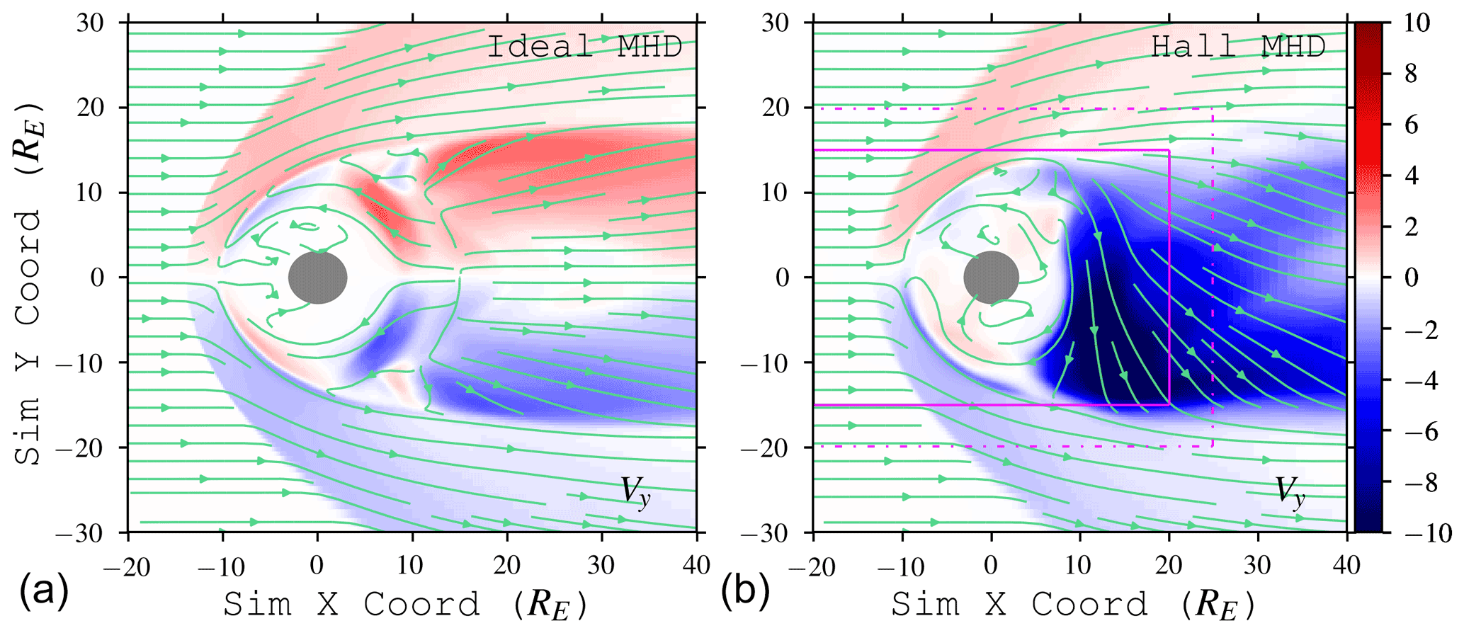
Figure 1 Cross-tail velocity V_y in the tail plane perpendicular to reconnection for both ideal (a) and Hall (b) MHD, normalized to v₀=97.9 km s⁻¹. Streamlines show in-plane velocity. Purple lines in the right figure surround the highest resolution regions: $\mathrm{\Delta }x,\mathrm{\Delta }y=\mathrm{0.2}$ R_E (solid); $\mathrm{\Delta }x,\mathrm{\Delta }y\le \mathrm{0.515}$ R_E (dot-dashed). A typical Dungey-like, symmetric convection pattern induced by numerical resistivity is clearly demonstrated in ideal MHD. Adding the Hall term induces out-of-reconnection-plane flows, which drives an asymmetric convection pattern; this is similar to what has been simulated for Ganymede (Dorelli et al., 2015; Tóth et al., 2016; Wang et al., 2018).

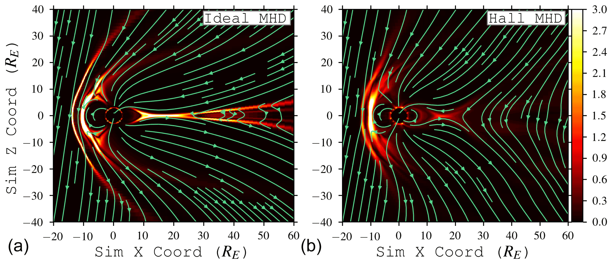
Figure 2 Normalized current density magnitude $\Vert J\Vert$ in the simulation xz plane at y=0 for both ideal (a) and Hall (b) MHD. Streamlines show in-plane magnetic field. Adding the Hall term induces out-of-reconnection-plane flows (Fig. 1); the resulting tail convection causes the magnetotail current sheet to vary along the x direction across the tail width (y) (see, e.g., Figs. 7 and 9 for examples of $\Vert J\Vert$ spatial variation in the xy plane).

3 Problem initialization

For our simulation setup, we choose normalized solar wind and terrestrial magnetic field parameters such that the magnetopause standoff distance matches that of Earth's magnetosphere (≈10 R_E), the bow shock standoff distance is ≈3 R_E beyond the magnetopause, and δ_i is equivalent to the planetary radius.

These relative distances can be controlled by setting four dimensionless parameters¹:

1. $M_{\mathrm{A}}=v_{\mathrm{sw}}/v_{\mathrm{A},\mathrm{sw}}$, the solar wind Alfvénic Mach number;

2. ${\mathit{\beta }}_{\mathrm{sw}}=\mathrm{8}\mathit{\pi }{P}_{\mathrm{sw}}/B_{\mathrm{sw}}^{\mathrm{2}}$, the solar wind plasma beta;

3. $\Vert B_{\mathrm{0}}\Vert /\Vert B_{\mathrm{sw}}\Vert$, the ratio of the dipole field strength at 1 R_E to the solar wind magnetic field;

4. ${\stackrel{\mathrm{‾}}{\mathit{\delta }}}_{\mathrm{i}}$, the ion inertial length.

Since only the first three of these parameters control the magnetopause and bow shock standoff distances, we can arbitrarily set δ_i to control the relative Hall scale. This allows our theoretical magnetosphere to be simultaneously “Earth-like” (in a relative physical sense) and ion-scale (relative to δ_i).

.

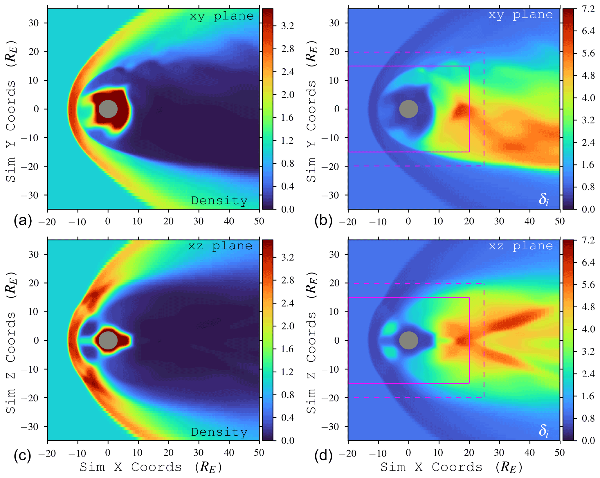
Figure 3 Density (a, c) and local value of δ_i (b, d) calculated via ${\mathit{\delta }}_{\mathrm{i},\mathrm{local}}=\sqrt{\mathrm{1}/\mathit{\rho }}$ in the xy (a, b) and xz planes (c, d), taken from an example snapshot during the final Hall MHD portion of the run. Density is normalized via $n_{\mathrm{0}}=\mathrm{5}{\mathrm{cm}}^{-\mathrm{3}}$ and m_i=3942 amu; δ_i is normalized via L₀=R_E. Purple lines denote same regions as Fig. 1: solid lines denote region with $\mathrm{\Delta }x,\mathrm{\Delta }y,\mathrm{\Delta }z=\mathrm{0.2}$ R_E; dashed lines denote $\mathrm{\Delta }x,\mathrm{\Delta }y,\mathrm{\Delta }z\le \mathrm{0.515}$ R_E. Most of the near-tail region (within purple boxes; x>0) has >5 cells per local δ_i

Thus, we choose our reference values as follows: $L_{\mathrm{0}}=R_{\mathrm{E}}=\mathrm{6.371}\times {\mathrm{10}}^{\mathrm{8}}\mathrm{cm}=\mathrm{6371}$ km, n₀=5 cm⁻³, ρ₀=m_in₀ with the mass of each ion $m_{\mathrm{i}}=\mathrm{6.546}\times {\mathrm{10}}^{-\mathrm{21}}\mathrm{g}=\mathrm{3942.18}\mathrm{amu}$, and $B_{\mathrm{w}}={\mathrm{10}}^{-\mathrm{4}}\mathrm{G}=\mathrm{10}$ nT. From these, we derive $v_{\mathrm{0}}=\mathrm{97.5}\times {\mathrm{10}}^{\mathrm{5}}\mathrm{cm}{\mathrm{s}}^{-\mathrm{1}}=\mathrm{97.5}\mathrm{km}{\mathrm{s}}^{-\mathrm{1}}$, t₀≈65 s, $P_{\mathrm{0}}=\mathrm{7.96}\times {\mathrm{10}}^{-\mathrm{10}}\mathrm{Ba}=\mathrm{0.0796}\mathrm{nPa}$, and ${\mathit{\delta }}_{\mathrm{i}}=\mathrm{6371}\mathrm{km}=\mathrm{1}{L}_{\mathrm{0}}=\mathrm{1}$ R_E.

The solar wind is initialized with values ρ_sw=1 ρ₀, $v_{\mathrm{sw}}=\mathrm{4.09}{v}_{\mathrm{0}}=\mathrm{400}$ km s⁻¹, and wind plasma β_sw=0.305 such that P_sw=0.1526 P₀. The wind magnetic field is initially set to B_sw=(-$\mathrm{0.174},\mathrm{0},\mathrm{0.985})B_{\mathrm{w}}$ for a northward interplanetary magnetic field (IMF) with magnitude B_sw=1 B_w; we later flip the IMF by setting $B_z=-\mathrm{0.985}$.

The planetary background magnetic field (B₀) is approximated with a magnetic dipole

$$\begin{array}{}\text{(10)}& {\displaystyle }{\mathit{B}}_{\mathrm{0}}={\displaystyle \frac{\mathrm{3}(\mathit{m}\cdot \mathit{r})\mathit{r}-\mathit{m}\Vert r{\Vert }^{\mathrm{2}}}{\Vert r{\Vert }^{\mathrm{5}}}},\end{array}$$

with r the position vector from the center at $(\mathrm{0},\mathrm{0},\mathrm{0})$ and the planetary dipole moment $\mathit{m}=(M_x,M_y,M_z)$ taken as (0, 0, −3000), such that $\Vert B_{\mathrm{0}}\Vert =\mathrm{3000}{B}_{\mathrm{w}}=\mathrm{0.3}\mathrm{G}$ on the magnetic equator at r=1 R_E. This satisfies the requirement that B₀ be both curl-free and divergence-free.

Figure 4 Cross-tail convection in the reconnection plane at z=0 for ions (a) and electrons (b), with the background color (orange) illustrating normalized current sheet density magnitude. Blue (green) streamlines indicate direction of electron (ion) velocity (normalized via $v_{\mathrm{0}}=\mathrm{97.9}\mathrm{km}{\mathrm{s}}^{-\mathrm{1}}$), with line sizes proportional to the magnitude of the maximum electron (ion) velocity in the plane. The electron velocity (in normalized units) is calculated from ${\mathit{v}}_e=\mathit{v}-\mathit{J}/\mathit{\rho }$.

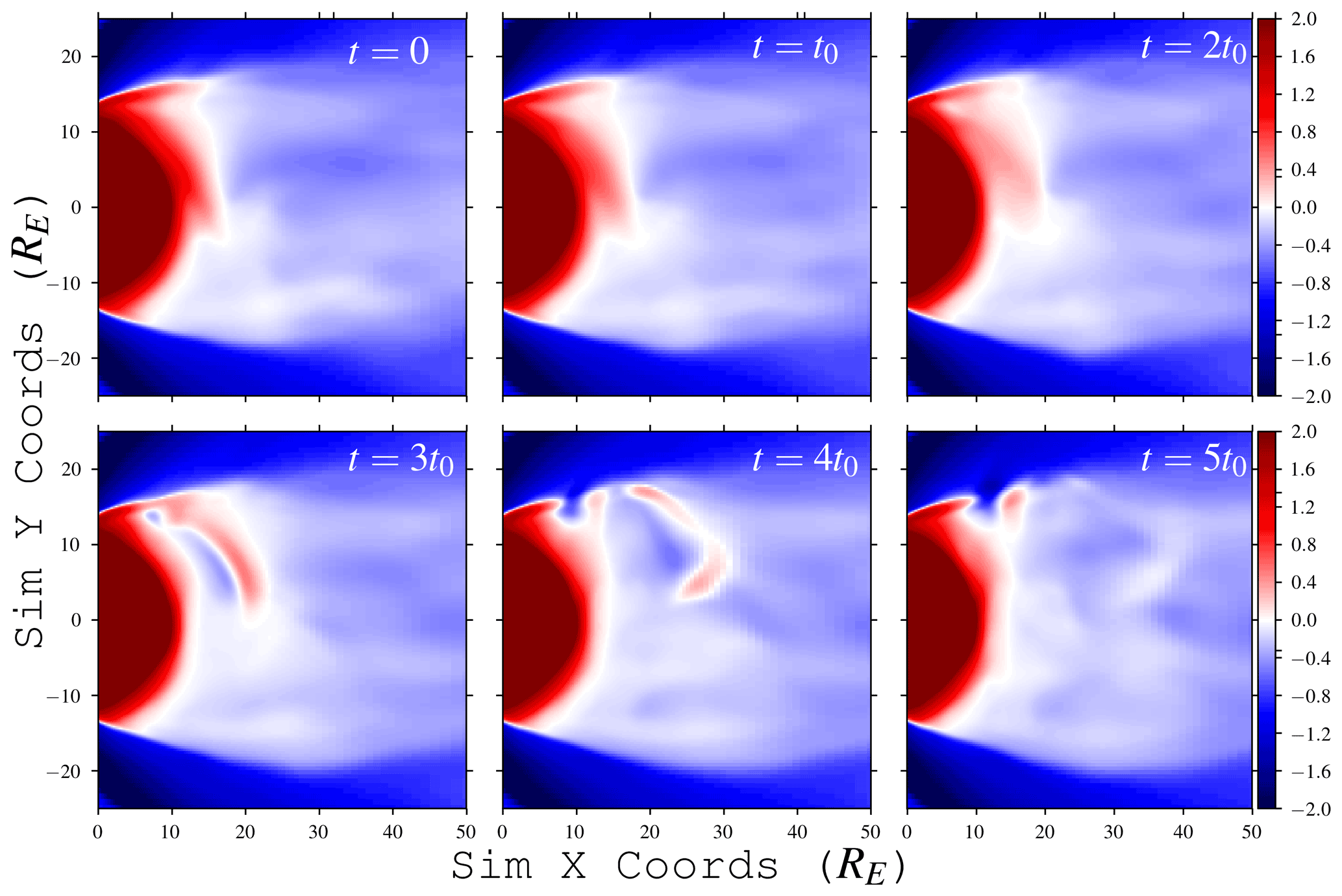
Figure 5 Formation and evolution of a global dipolarization over 5 t₀≈5.4 min, as seen in the evolution of magnetotail normal magnetic field B_z (red: out-of-page; blue: into page). Displayed times are relative to upper left image; t=0 here corresponds to 6t₀ after the start of the 45 t₀ Hall MHD simulation period. B_z has been normalized via $B_{\mathrm{w}}={\mathrm{10}}^{-\mathrm{4}}\mathrm{G}$.

As a summary, the dimensionless parameters for this experimental magnetosphere are M_A=4.09; β_sw=0.305; $\Vert B_{\mathrm{0}}\Vert /\Vert B_{\mathrm{sw}}\Vert =\mathrm{3000}$; ${\stackrel{\mathrm{‾}}{\mathit{\delta }}}_{\mathrm{i}}=\mathrm{1}$. For Earth, ${\stackrel{\mathrm{‾}}{\mathit{\delta }}}_{\mathrm{i}}\approx \mathrm{1}/\mathrm{70}$ and the other parameters would be the same. For Mercury, the dimensionless parameters would be, e.g., $M_{\mathrm{A}}=\mathrm{6}.$; β_sw=0.65; $\Vert B_{\mathrm{0}}\Vert /\Vert B_{\mathrm{sw}}\Vert =\mathrm{15}$; ${\stackrel{\mathrm{‾}}{\mathit{\delta }}}_{\mathrm{i}}=\mathrm{1}/\mathrm{65}$.

At the inner boundary, we had difficulties with density depletion causing large local Alfvén speeds and small global time steps. We tried several types of inner boundaries, experimenting with different combinations of floating (zero-gradient) and fixing the plasma variables. Ultimately, although the following inner boundary conditions are not entirely realistic, they allow for a stable evolution of the magnetosphere in both the dayside and the tail. We set the inner boundary at a radius of 3 R_E; in these ghost cells, we fix the density at 4 ρ₀, float the pressure, float the radial magnetic field, set the tangential B to zero, and set the velocity to zero. For the divergence cleaning, we find that simply setting the ghost ψ_c = 0 works better than having a floating condition. We note that in more realistic magnetospheres, cold plasma from the ionosphere may flow out to the tail and impact the dynamics. We will leave this topic for future studies.

For the outer boundaries, the left edge of the simulation domain fixes the conservative variables to the background solar wind condition; the rest of the box has zero-derivative boundaries for all variables.

The simulation coordinates are defined with −x pointing towards the Sun, z along the planetary magnetic dipole axis, and +y (−y) towards the dusk (dawn) completing the orthogonal set. Although the planet does not rotate, dawn and dusk are used assuming the sun rises in the east. In order to resolve the artificially inflated δ_i, we choose 5 cells per ${\stackrel{\mathrm{‾}}{\mathit{\delta }}}_{\mathrm{i}}$, giving a minimum resolution of $\mathrm{\Delta }x,\mathrm{\Delta }y,\mathrm{\Delta }z=\mathrm{0.2}$ R_E. This resolution is set within the range −20 R_E < x<20 R_E; −15 R_E < y, z<15 R_E; beyond this the cell length increases by 7 % with each additional cell up to a maximum of 5 R_E or until it hits the boundary. The total size of the grid is $\mathrm{290}\times \mathrm{253}\times \mathrm{253}$ (just over 18 million cells), covering a domain of −35.6 R_E < x<122 R_E, −86.4 R_E < y, z<86.4 R_E.

We start the simulation in ideal MHD (${\stackrel{\mathrm{‾}}{\mathit{\delta }}}_{\mathrm{i}}=\mathrm{0}$) with a northward IMF (B_sw given above) for 120 t₀ and then flip B_z,sw for the southward IMF case and run it for another 120 t₀. At this point, we turn on the Hall term by setting ${\stackrel{\mathrm{‾}}{\mathit{\delta }}}_{\mathrm{i}}=\mathrm{1}$ and run it for another 12 t₀ in order to allow the perturbations induced by the abrupt change of physics to settle. From this point on, the simulation was run for 45 t₀ under continuous pure southward IMF and with the Hall term on. The main results discussed below come from this final portion of the run with the Hall term enabled.

4 Results and discussion

4.1 Hall-induced asymmetry

Prior to turning on the Hall term, the magnetospheric convection is of Dungey-type. Turning the Hall term on, however, induces an out-of-reconnection-plane E×B force which breaks that symmetry and drives convection in a preferred direction (Fig. 1). This convection also modifies the current sheet structure between ideal and Hall MHD (Fig. 2) and causes it to vary in length along the x− direction across the tail y coordinate. For smaller magnetospheres, this effect was first seen in nonideal MHD simulations of Ganymede (Dorelli et al., 2015; Tóth et al., 2016; Wang et al., 2018); this was later seen in 10-moment and embedded kinetic simulations of Mercury (Dong et al., 2019; Chen et al., 2019). Our simulation supports the idea that this Hall-induced drift is sufficient to produce an asymmetry: kinetic effects are not required, but they may manifest different kinds of asymmetry.

Finally, since our choice of $min\mathrm{\Delta }x,\mathrm{\Delta }y,\mathrm{\Delta }z=\mathrm{0.2}$ R_E is based on the normalized δ_i=1 R_E, we check here that we are able to correctly resolve δ_i in the tail. As Fig. 3 illustrates, the local value of δ_i exceeds 1 R_E in the magnetotail and may reach up to 5 R_E. Thus, we are appropriately resolving the Hall length scales in the tail.

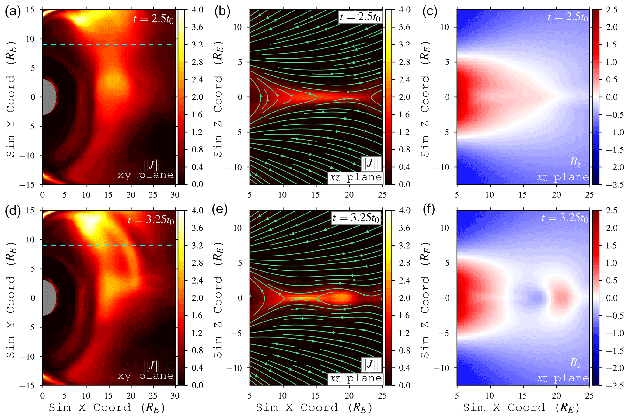
Figure 6 Formation and evolution of a global dipolarization due to locally reconnecting magnetic field lines in the xy and xz planes, as seen in the evolution of magnetotail current density ($\Vert J\Vert$) and normal magnetic field B_z. $\Vert J\Vert$ is normalized via $J_{\mathrm{0}}=B_{\mathrm{w}}/L_{\mathrm{0}}$; B_z is normalized via $B_{\mathrm{w}}={\mathrm{10}}^{-\mathrm{4}}\mathrm{G}$. Displayed times are relative to the sequence shown in Fig. 5. The dashed cyan lines in (a) and (d) mark the y position of the xz cuts in (b), (c), (e), and (f).

Figure 7 Example of B_x sampling and Harris sheet fit (b) as described in text (Eq. 11). χ²=0.004 for this fit. B_x has been normalized via $B_{\mathrm{w}}={\mathrm{10}}^{-\mathrm{4}}\mathrm{G}$. Panel (a) shows the magnetotail current sheet magnitude (normalized via $J_{\mathrm{0}}=B_{\mathrm{w}}/L_{\mathrm{0}}$) in the simulation z=0 plane; the B_x sampling box domain boundaries are shown in cyan, with the small cross showing the location of the example sample. The box boundaries are $\mathrm{12}<x<\mathrm{16}$ and $-\mathrm{15}<y<\mathrm{15}$.

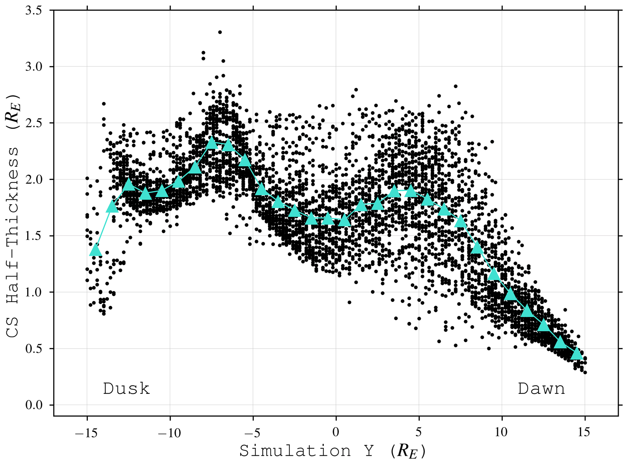
Figure 8 Best-fit current sheet half-thicknesses (L_CS) derived by fitting Eq. (11) to 5037 cuts of B_x along the z direction. These cuts were randomly sampled in the tail xy plane and over the simulation time period (see text). There is a bias towards the current sheet being thinner on the dawnside. However, the dawnside also sees a larger spread in thicknesses: this is a result of temporal effects (see main text for discussion).

4.2 Dipolarizations

In our simulation, the Hall electric field induced by tail reconnection accelerates ions towards the duskside and the electrons towards dawn. Since δ_i=R_E here, the reconnection current sheet spans a significant fraction across the tail; this means that the ions are decoupled from the magnetic field during much of their in-plane convection duskward (green arrows in Fig. 4). The electrons, being coupled to the magnetic field, carry the reconnected, normal B_z flux dawnward (blue arrows). Because the reconnected magnetic flux originates over a large region within the tail, there is a significant pileup leading to a reconnecting, active region of plasmoid formation on the dawnside. This pileup–reconnection mechanism may be a general cause of dipolarizations in ion-scale magnetospheres (like Mercury, e.g., Sundberg et al., 2012). Although the drifting electrons themselves do not cause dipolarization events, they can affect where events occur. We speculate that increasing the system size relative to δ_i will limit the extent of dawnward flux transport via current sheet electrons and cause the flux pileup to shift closer to tail center (or duskward). In other words, this type of asymmetry we observe here may be more pronounced in δ_i-scale magnetospheres and weaker in larger magnetospheres. However, it is unknown how this mechanism will interact with the overall Hall-induced duskward ion convection, which will begin to dominate electron convection at scales ≫δ_i.

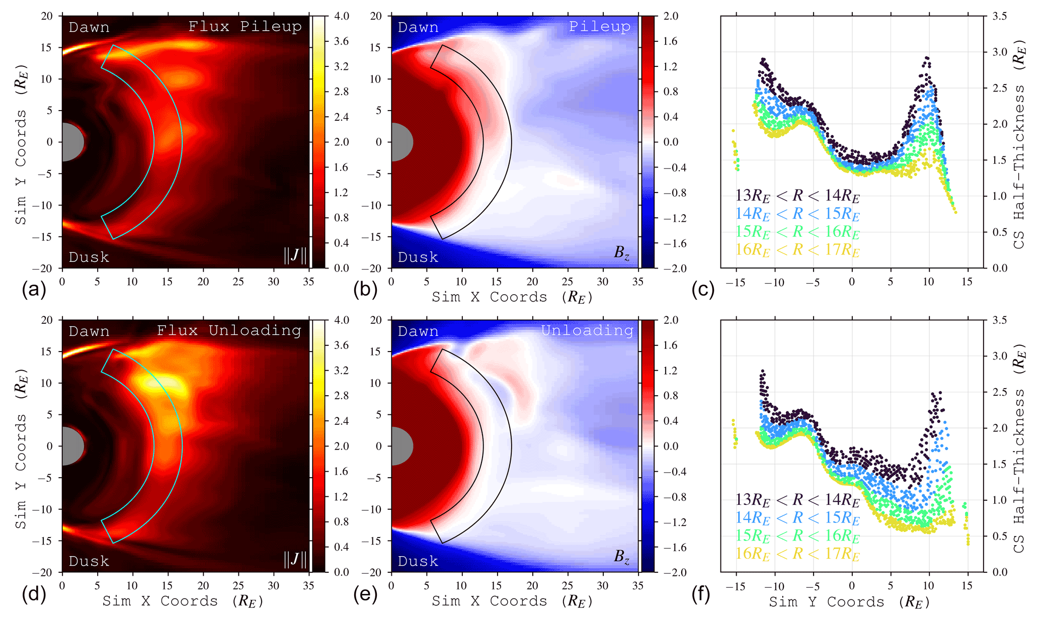
Figure 9 Cross-comparison of current sheet density magnitude (a, d), current sheet B_z flux pileup (b, e; same parameters as Fig. 5) and sampled thicknesses (c, f) during (a, b, c) and after (d, e, f) a global dipolarization event. Current sheet fits are sampled from the area within the wedges (13 R_E < R<17 R_E). The current sheet is thick where the B_z flux has piled up and thin where the flux has been unloaded. There is a 2.25 t₀≈2.4 min time difference between the snapshots of the top and bottom rows.

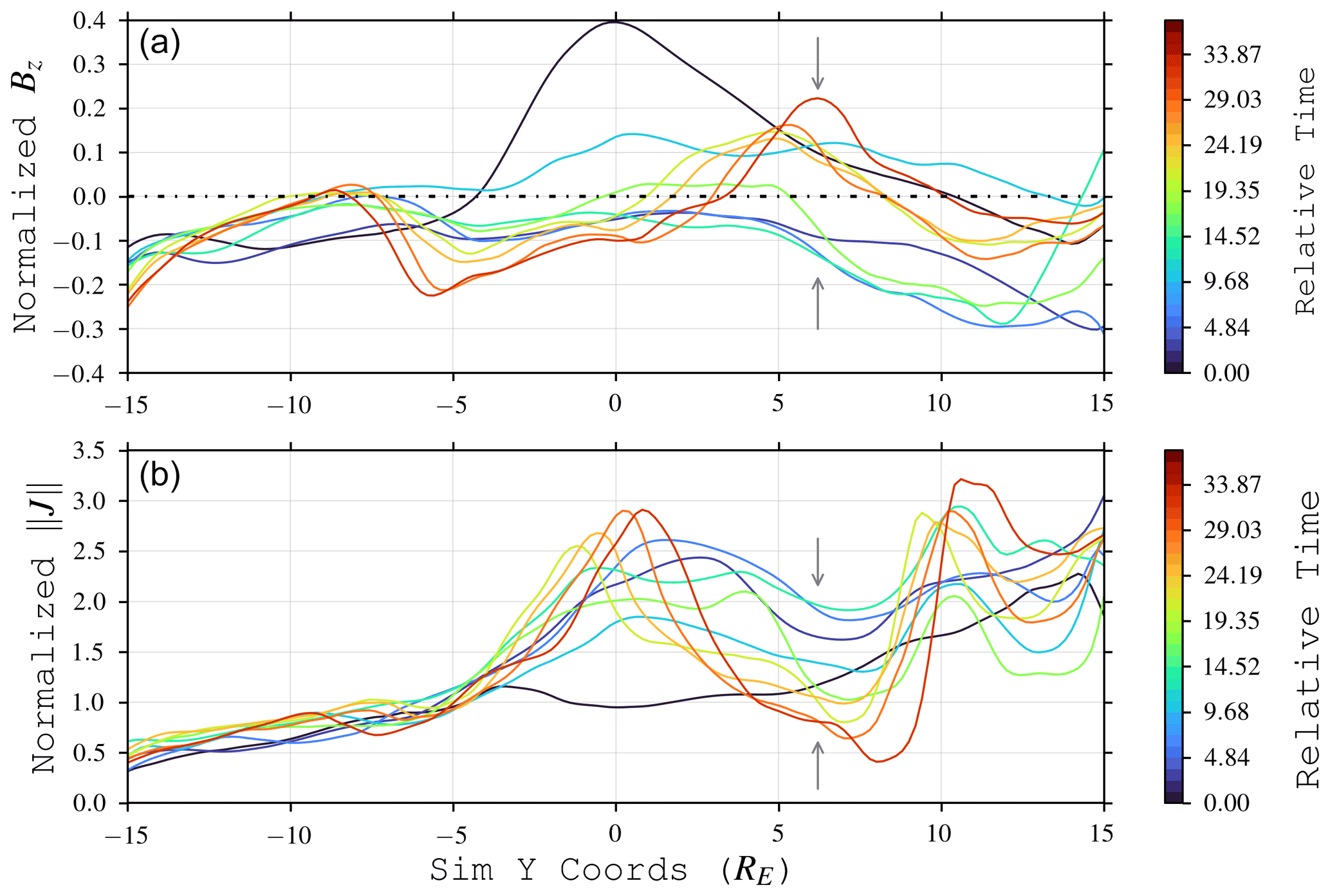
Figure 10 1D cuts of tail magnetic field B_z (a) and current density magnitude $\Vert J\Vert$ (b) taken from x=15 R_E, −15 R_E < y<15 R_E in the z=0 equatorial plane. $\Vert J\Vert$ is normalized via $J_{\mathrm{0}}=B_{\mathrm{w}}/L_{\mathrm{0}}$; B_z is normalized via $B_{\mathrm{w}}={\mathrm{10}}^{-\mathrm{4}}\mathrm{G}$. Colors denote times relative to t=0 in Fig. 5 (top left panel). Arrows highlight where local pileup of B_z on dawnside thickens the current sheet, resulting in a lower current density and impeding local reconnection.

During the 45 t₀ ≈48 min duration of our simulation, there were seven events visually observed on the dawnside (none on the duskside) which followed the general substorm pattern of a buildup/loading phase followed by an unloading (or expansion/relaxation) phase (Rostoker et al., 1980). For each event, we observed pileup of the normal B_z magnetic flux over a period of several minutes, followed by a burst of reconnection and the subsequent ejection of plasmoids tailward (Figs. 5 and 6). Three of the seven events produced large plasmoids (on the order of 10 R_E = 10δ_i), while the rest resulted in smaller ones (≤5 R_E; ≤5δ_i). The larger ejecta appeared to build up and release on timescales of around 10 min, while the smaller events had shorter timescales of around 5 min. Most events originated at a down-tail distance ≈13–16 R_E; after ejection, their resulting plasmoids traveled to about 30 R_E down-tail over several minutes before dissipating.

The observed dawnward bias in dipolarization events for our ion-scale magnetosphere corroborates similar dawnward biases found in MESSENGER observations (Sun et al., 2016; Dewey et al., 2018) and global simulations of Mercury (Dong et al., 2019; Chen et al., 2019). It is interesting to note that our results are under a steady, southward solar wind condition. As long as there is Hall-driven convection in the tail, the competition between dawnside B_z pileup and reconnection drives this cycle. At the moment, it is not clear whether this process is unique to our ion-scale Earth, since its strong planetary dipole field means that flux piles up over a large swath of the tail. It is possible that a similar process may occur at Mercury (which has a weaker dipole field), i.e., that its observed dipolarizations are indeed akin to global substorms (Kepko et al., 2015). Further investigation is needed to determine how varying the magnetospheric parameters (as presented in Sect. 3) affects these observations, especially as system size increases relative to δ_i.

We note that, at Earth, there are additional localized (not global) dipolarization fronts resulting from current sheet instabilities or transient reconnection events (e.g., Runov et al., 2009; Sitnov et al., 2009). We do not see these small-scale fronts in our ion-scale Earth; this may be because we do not have enough down-tail resolution to observe localized current sheet instabilities which form them.

4.3 Current sheet thickness

Another test of the active region picture is the predicted thickness asymmetry of the tail current sheet: Liu+ predicted that the sheet would be thinner on the dawnside. We follow Poh et al. (2017a) and estimate the current sheet thickness in our model by using a Harris sheet (Harris, 1962):

$$\begin{array}{}\text{(11)}& {\displaystyle }{B}_x=B_{\mathrm{a}}\tanh {\displaystyle \frac{Z-Z_{\mathrm{0}}}{L_{\mathrm{CS}}}}+\text{offset},\end{array}$$

where B_a is the asymptotic lobe field, Z₀ is the current sheet center, L_CS is the current sheet half-thickness, and the offset allows for asymmetry between the north and south B_x lobes on either side of the current sheet. We take 6000 one-dimensional cuts of B_x along the north–south direction between $z=\pm \mathrm{10}$ R_E in a volume covering the current sheet from 12 R_E < x<16 R_E and −15 R_E < y<15 R_E, randomly sampled across the box plane and during the final 45 t₀≈48 min period (example shown in Fig. 7). These cuts are fit to Eq. (11) using the Levenberg–Marquardt least-squares algorithm in scipy.curvefit (Virtanen et al., 2020); instances that do not fit well (χ²>0.01) or that return nonsensical results (L_CS<0) are rejected. This results in 5037 samples of the current sheet thickness across the magnetotail (Fig. 8). This distribution shows that the dawnward current sheet is thinner on average than the duskward sheet. However, there is a significant scatter in this result; the dawn sheet covers a wider range of thicknesses. This variation is caused by the dawnside pileup–reconnection mechanism.

The current sheet oscillates with the dipolarization cycle (Sect. 4.2) between a “thick state” due to the B_z pileup and a “thin state” immediately following the flux unloading and plasmoid ejection. This is demonstrated in Fig. 9, where fitted CS thicknesses during both flux loading and unloading stages are plotted along with snapshots of the B_z state. During the loading stage, the piled up flux on the dawnside (5 R_E < y<12 R_E) fattens the current sheet; here, the sampled dawn thicknesses are comparable to and can exceed the dusk thicknesses. However, after the unloading stage, the current sheet on the dawnside is much thinner where the flux has been evacuated (bottom right plot; R>15 R_E). Interestingly, we can see that where the B_z flux remains (R<15 R_E), the current sheet continues to be thick. Combining all the sample fits over several cycles of loading and unloading results in the picture shown in Fig. 8: a dawnward current sheet moving between thick and thin states depending on the level of flux pileup. Indeed, this is a common pattern throughout the simulation: where there is flux pileup, the current sheet is thicker, and the current density is lower (e.g., Fig. 10).

This cycle may explain the apparent contradiction between the Liu+ prediction of thinner dawnward current sheets in ion-scale magnetospheres and the Poh et al. (2017b) spacecraft observation of thicker dawnward sheets at Mercury. Even though, on average, the current sheet is thinner dawnward (as Liu+ predicts), the sampling of measurements could be producing the opposite result. As shown in Figs. 8 and 9, the sampled sheet thickness can greatly depend on where and when the craft crosses the tail. In our simulation, the current sheet is continuously morphing between thick and thin states; both types of regions exist simultaneously within the dawnside. Most points in the tail preferentially see thicker sheets over time, though some preferentially see thinner sheets. It is possible that these effects combine to produce a sampling bias in time and space towards thicker sheets. We note that this is speculation and will require more investigation with respect to the various solar wind driving conditions and seasons that MESSENGER experiences at Mercury.

5 Conclusions

We have simulated a small, ion-scale Earth in which the standoff distance and magnetotail width are akin to Earth's as measured in planetary radii but with the solar wind ion-scale length δ_i set to 1 R_E. The resulting tail plasma behavior was more similar to Mercury's magnetosphere than Earth's. Along with Chen et al. (2019) and Dong et al. (2019), our results support the idea that tail asymmetry is a universal consequence of the Hall effect in ion-scale magnetospheres. Essentially, it is the relative size of the magnetosphere compared to δ_i, not the absolute size (planetary radii), that controls the importance and influence of Hall-induced consequences. We find that Hall effects are sufficient to generate tail asymmetries in dipolarization, plasmoids, and current sheet thickness. No electron-scale kinetic effects are required, though they may contribute to or modify asymmetries. However, we emphasize that we did not simulate the same magnetosphere as Chen et al. (2019): our ion-scale Earth is smaller relative to δ_i than Mercury and has different magnetospheric parameters (Sect. 3). There may be additional effects not being considered, especially with regards to how varying the dimensionless magnetospheric parameters affects the manifestation of tail asymmetries.

In general, our simulation appears to corroborate the Liu+ picture of tail asymmetry in ion-scale magnetospheres; however, the Lu+ finding that the transported tail B_z thickens the current sheet is readily manifested here. Although the reconnected B_z does drive outflows and thin current sheets on the dawnside, we see that it can pile up and thicken current sheets. There is a continuous cycle between the dawnward transport of B_z leading to pileup (which thickens the current sheet) and reconnection (which thins the current sheet); this manifests in an oscillating current sheet thickness. On average, we find the current sheet is thinner on the dawnside, but it can occasionally be thicker in some regions depending on the level of flux pileup.

Further study will be required to confirm or contrast this picture for magnetospheres with system size ≫ δ_i. Since our simulation is of a experimental magnetosphere, several questions concerning more realistic magnetotails remain:

• How does the weaker, offset dipole of Mercury affect the amount of magnetic flux available for transport/pileup and the resulting plasmoid formation/ejection?

• Are the observed dipolarizations at Mercury actually “global”, like substorms?

• How does increasing the system size $/$ δ_i ratio affect asymmetry formation, tail convection, transport of B_z, and plasmoid and DF formation?

• What other effects (e.g., kinetic, ionosphere) cause asymmetries, and how do they interact with the Hall effect and one another?

We look forward to future studies which will investigate these questions in greater detail.