Fine-scale dynamics of fragmented aurora-like emissions

Fragmented aurora-like emissions (FAEs) are small (few kilometres) optical structures which have been observed close to the poleward boundary of the aurora from the high-latitude location of Svalbard (magnetic latitude 75.3 ^∘N). The FAEs are only visible in certain emissions, and their shape has no magnetic-field-aligned component, suggesting that they are not caused by energetic particle precipitation and are, therefore, not aurora in the normal sense of the word. The FAEs sometimes form wave-like structures parallel to an auroral arc, with regular spacing between each FAE. They drift at a constant speed and exhibit internal dynamics moving at a faster speed than the envelope structure. The formation mechanism of FAEs is currently unknown.

We present an analysis of high-resolution optical observations of FAEs made during two separate events. Based on their appearance and dynamics, we make the assumption that the FAEs are a signature of a dispersive wave in the lower E-region ionosphere, co-located with enhanced electron and ion temperatures detected by incoherent scatter radar. Their drift speed (group speed) is found to be 580–700 m s⁻¹, and the speed of their internal dynamics (phase speed) is found to be 2200–2500 m s⁻¹, both for an assumed altitude of 100 km. The speeds are similar for both events which are observed during different auroral conditions. We consider two possible waves which could produce the FAEs, i.e. electrostatic ion cyclotron waves (EIC) and Farley–Buneman waves, and find that the observations could be consistent with either wave under certain assumptions. In the case of EIC waves, the FAEs must be located at an altitude above about 140 km, and our measured speeds scaled accordingly. In the case of Farley–Buneman waves a very strong electric field of about 365 mV m⁻¹ is required to produce the observed speeds of the FAEs; such a strong electric field may be a requirement for FAEs to occur.

1 Introduction

Unusual optical phenomena in the polar upper atmosphere have recently been reported which are aurora-like but do not appear to be caused by energetic electron or proton precipitation; therefore, the term aurora cannot be applied to them. The subject of this work is one such type of structure, first reported by Dreyer et al. (2021) and named fragmented aurora-like emissions (FAEs). FAEs appear as small (a few kilometres at an assumed altitude in the lower E region) fragments of green emission in colour all-sky camera images. They exhibit a lack of extent in the magnetic-field-aligned direction, short lifetimes of less than a minute, and, so far, have only been observed during auroral activity. Dreyer et al. (2021) identified two categories of FAEs; the first category consists of individual or irregularly spaced fragments, while FAEs in the second category form wave-like structures with regular spacing between them. Another feature of FAEs is that they have been observed close to the poleward boundary of the auroral oval, i.e. at very high latitudes. The mechanism producing the fragments is not yet known, but Dreyer et al. (2021) suggested the Farley–Buneman instability may be responsible.

Another type of aurora-like emission, which has recently received considerable interest, is Strong Thermal Emission Velocity Enhancement (STEVE). STEVE is an east–west band of emission occurring at subauroral latitudes in a region of high electron temperature and fast westward moving hot ions (MacDonald et al., 2018; Gallardo-Lacourt et al., 2018; Archer et al., 2019). The optical spectrum of STEVE, in particular the lack of emission in N${}_{\mathrm{2}}^{+}$ 1N and OI 557.7 nm, suggests that it is not a result of auroral particle precipitation (Gillies et al., 2019). Dreyer et al. (2021) used a similar argument to conclude that FAEs are not likely to be directly caused by particle precipitation.

STEVE can be accompanied by a magnetic-field-aligned green rayed arc called the picket fence. Despite its clear association with the magnetic field, Gillies et al. (2019) did not observe emission in N${}_{\mathrm{2}}^{+}$ 1N at 427.8 nm, which Mende et al. (2019) used as evidence to conclude that, like STEVE, the picket fence is not produced by energetic particle precipitation. The mechanism producing the picket fence is currently unknown.

Semeter et al. (2020) analysed streaks of green emission between STEVE and the picket fence and found that they occur in the lower E-region ionosphere at an altitude of 103–108 km. The streaks had no clear orientation with respect to the magnetic field, and morphological considerations led the authors to conclude that the streaks are not caused by precipitation and are, instead, a result of direct excitation by suprathermal electrons in the ionosphere. Streaks look similar to FAEs, they have similar lifetimes, and their scale sizes are also similar, although it is not clear whether their internal dynamics are exactly the same. It is possible that streaks and FAEs are produced by a similar, or even the same, physical process on opposite sides (poleward and equatorward) of the auroral oval.

An auroral form named dunes was reported by Palmroth et al. (2020), using observations made by citizen scientists with off-the-shelf camera equipment. The dunes appear as a monochromatic horizontal wave with a wavelength of about 45 km, parallel to and equatorward of a bright auroral arc, such that each dune is a finger-like projection of emission from the arc. It was found that the dunes are constrained to a narrow altitude range around 100 km. The authors suggest the dunes may be a signature of a mesospheric bore which modulates the atomic O density, although they do not rule out that the oscillation comes from a variation in the electron precipitation source. Based on the thin altitudinal extent and the lack of any field-aligned structure, a similar argument may apply to dunes as that made by Semeter et al. (2020) to streaks; this means that the dune emission is not a direct result of particle precipitation and is, instead, caused by local energisation of the plasma and, therefore, may not be aurora in the normal sense of the word. Dunes have morphological similarities to the second category of FAE, which also forms waves adjacent to an auroral arc, but the scale sizes are very different. Dreyer et al. (2021) found that FAEs are typically a few kilometres long, with a similar distance separating them; dunes are roughly an order of magnitude larger than FAEs. To our knowledge, there are no optical observations of dunes with sufficient spatial and temporal resolution to establish whether or not they have similar internal dynamics to FAEs.

Here we analyse two FAE events in detail using high-resolution optical observations made in the high Arctic at the poleward boundary of the auroral oval. The first event occurred on 4 December 2013 and consists of FAEs from the second category, i.e. those forming a wave-like structure adjacent to an auroral arc. The second event occurred on 22 December 2014 and was discovered by citizen scientists taking part in the Aurora Zoo project (https://www.zooniverse.org/projects/dwhiter/aurora-zoo, last access: 17 November 2021) to classify fine-scale aurora. Although the FAEs in the second event are adjacent to an auroral arc, they do not form a clear, monochromatic wave structure, and so they fall into the first category described by Dreyer et al. (2021). The FAEs in both events exhibit similar dynamics and internal structure.

Our observations and instrumentation are described in Sect. 2. We present an analysis to determine the drift speed of the FAEs and the speed of their internal dynamics in Sect. 3. Finally, we discuss the results and examine some possible theories for the generation mechanism of the FAEs in Sect. 4.

2 Instrumentation and observations

This work primarily uses data from the ASK (Auroral Structure and Kinetics) instrument, which consists of three coaligned EMCCD (electron multiplying charge coupled device) imagers pointed towards magnetic zenith. For this study, data from two of the imagers are used, which are equipped with filters with a passband centred at 673.0 nm for observations of emission from molecular nitrogen (N₂ 1P) and at 777.4 nm for observations of emission from atomic oxygen (OI). The field of view (FOV) of each imager is ${\mathrm{6.1}}^{{}^{\circ }}\times {\mathrm{6.1}}^{{}^{\circ }}$, corresponding to 10.7 by 10.7 km at 100 km altitude and centred on magnetic zenith. Each ASK imager recorded at 32 frames per second during event 1 and at 20 frames per second during event 2, with images captured simultaneously on all imagers. ASK is located at the European Incoherent Scatter Scientific Association (EISCAT) Svalbard Radar (ESR) at 78.2^∘ N, 16.1^∘ E (MLAT 75.3^∘ N). During event 1, ESR was running the experiment “beata”, which is a field-aligned alternating code experiment providing estimates of plasma parameters in the E and F regions at a temporal resolution of 6 s and range resolution down to 3.7 km. ESR was not operating during event 2. The all-sky data used in this study are from the University Centre in Svalbard (UNIS) colour digital SLR (single-lens reflex) camera with a fish-eye lens, which is installed at the Kjell Henriksen Observatory (KHO), 0.6 km from the ESR site.

Figure 1 Event 1 on 4 December 2013. The top row shows colour all-sky camera images, with the time at the start of the exposure given below each frame. The bottom row shows selected ASK images of N₂ 1P emission at 673.0 nm.

For event 1 on 4 December 2013, a substorm took place with an onset time at around 18:50 UT, when the aurora moved rapidly northwards and reached the high latitudes of ESR. The aurora formed several east–west-aligned dynamic arcs. The poleward boundary of the aurora reached magnetic zenith at about 18:51 UT, and ASK observed aurora intermittently over a period of about 20 min. As the most poleward auroral arc passed through the ASK FOV at 19:04:06 UT from the north to the south, thin filamentary structures, which are regularly spaced and oriented in an almost completely north–south direction, were detected poleward of the boundary arc. These structures are FAEs. A sequence of all-sky images from the event are shown in the top row of Fig. 1, and a sequence of ASK images of N₂ 1P (673.0 nm) emission are shown in the bottom row. Note that the times of the all-sky and ASK images do not coincide, and the exposure time of the all-sky images (10–15 s) contains many ASK images. The ASK observations show that the FAEs are dynamic and exhibit internal structuring. A video of the sequence is available in the video supplement accompanying this article. It is important to note that the fragments are not ray-like structures directed towards the magnetic zenith. Instead, they keep their north–south-aligned direction as they drift through the ASK FOV, with the exception of the last filament (the one just left of centre in the last ASK image shown in Fig. 1), which tilts to the northeast–southwest as the auroral arc changes direction, as if to stay perpendicular to the arc. The FAEs are small and quite fast moving and are, therefore, blurred during the all-sky exposure time to the extent that they are not visible at all in the all-sky images. The focus of the all-sky images from this event is, unfortunately, not sufficient to resolve stars, and so they cannot be accurately geometrically calibrated, which precludes accurate comparison with the ASK images. However, we include the all-sky images to show the large-scale context and approximate location of the FAEs with respect to the aurora.

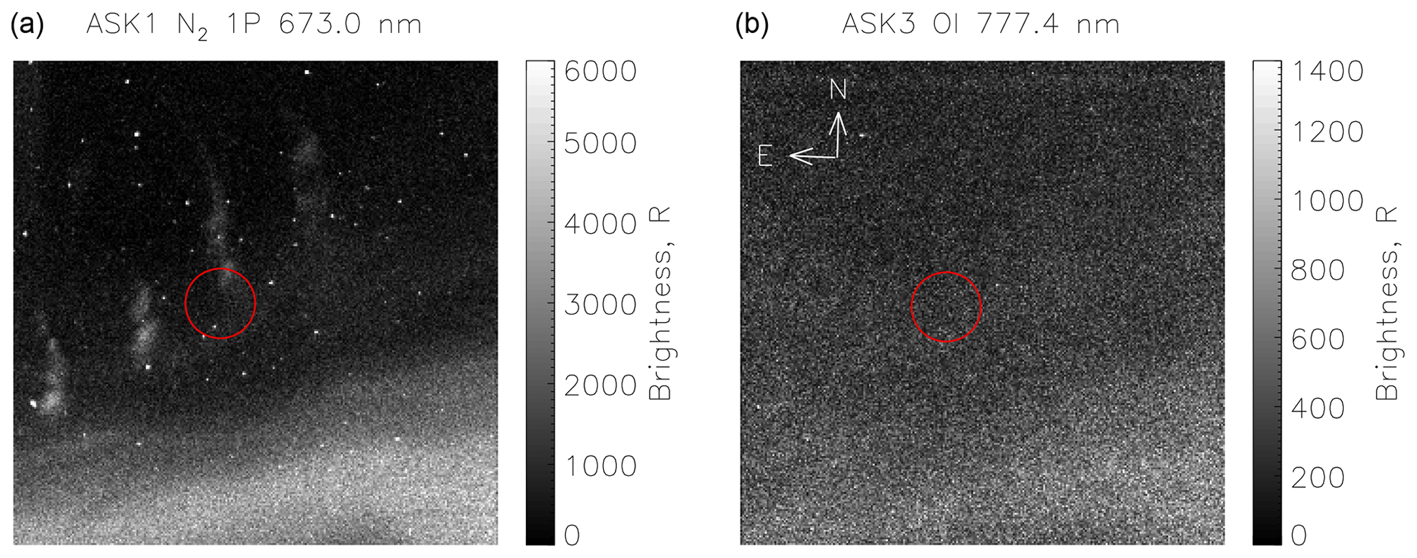
Figure 2 Simultaneous images in N₂ 1P (a; ASK1) and OI 777.4 nm (b; ASK3) at 19:04:15.438 UT during event 1. The FAEs are visible in N₂ 1P, whereas only the auroral arc is visible in OI 777.4 nm across the bottom right of the image. The full width at half maximum of the ESR beam is shown as a red circle in both images.

Figure 2 shows coincident images from ASK1 (left; N₂ 1P; 673.0 nm) and ASK3 (right; OI; 777.4 nm) at 19:04:15.438 UT, close to the middle of event 1. The full width at half maximum of the radar beam is plotted on the images as a red circle. The FAEs are seen as vertical (north–south) structures in the N₂ 1P image, but are not clearly visible in the OI (777.4 nm) emission. The auroral arc is seen across the bottom portion of both images. In N₂ 1P, the brightness of the FAEs is comparable to that of the auroral arc.

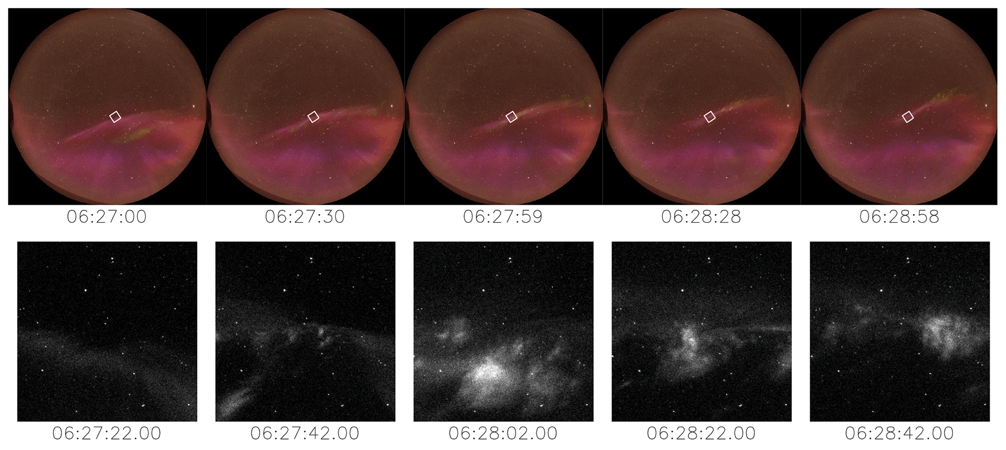
Figure 3 Event 2 on 22 December 2014. As for Fig. 1, the top row shows colour all-sky camera images, with the time at the start of the exposure given below each frame. The bottom row shows selected ASK images of the N₂ 1P emission at 673.0 nm. The ASK field of view is indicated in the all-sky images as a white box.

Figure 4 A portion of the colour all-sky image (a) corresponding to the ASK image in N₂ 1P recorded at 06:28:06.05 UT during event 2 (b). The location of the ASK field of view is indicated in the all-sky image as a white box. The ASK image is selected from the centre of the all-sky camera exposure time.

Event 2 is not associated with a substorm and, instead, involves a poleward-moving system of red rayed arcs of the type commonly observed in the morning cusp hours on Svalbard, associated with low-energy electron precipitation and possibly poleward-moving auroral forms (PMAFs). All-sky images and ASK images (N₂ 1P) of the event are shown in Fig. 3, and a video of the ASK data is available in the video supplement accompanying this article. The most poleward arc slowly passed through the ASK field of view between 06:27:00 and 06:29:30 UT, when FAEs were observed. The FAEs in event 2 are larger and brighter than the FAEs in event 1, and they are not north–south aligned, although their internal structuring and dynamics look similar. Because they are larger than the FAEs in event 1, in this case they are observed as green emission in the colour all-sky images, despite the motion blur, especially southward of the zenith arc in the image recorded at 06:27:00 UT. Figure 4 shows an enlarged portion of the all-sky image recorded at 06:27:59 UT (left), together with an ASK image from the midpoint of the all-sky exposure time (right). The ASK field of view is drawn on the all-sky image with a white box. The large bright FAE seen at the bottom right of the ASK image appears as a green blob in the colour all-sky image. The auroral arc has a pink colour in the all-sky image, with the green colour of the FAEs visible both equatorward and poleward of the arc.

In event 1, the FAEs are observed on the poleward side of the arc and drift eastward, while in event 2 the FAEs are observed in ASK on the equatorward side of the arc and drift westward. The all-sky camera images, however, show that the FAEs in event 2 moved from the equatorward side to the poleward side. Without ASK measurements from the poleward side, it is not possible to determine if the drift speed or direction changed as the FAEs crossed the arc, but the all-sky data show that the FAEs can exist on both sides of the arc. In event 1, the FAEs drift more slowly than the structure seen within the auroral arc, where intrinsic auroral features are estimated to move with speeds of up to 3.9 km s⁻¹. The aurora in event 2 is less dynamic, with fewer features than the aurora in event 1, but the FAEs drift at a comparable speed to the auroral features which are seen.

2.1 Ionospheric electrodynamics

The ESR was operating throughout event 1, providing measurements of electron density, electron temperature, and ion temperature. The top panel of Fig. 5 shows the electron density as a function of height and time, as measured by the ESR during 6 min from 19:00 UT on 4 December 2013. The enhancement near 19:03:00 UT and 100 km altitude is when the centre of the boundary arc passed through the radar beam as it drifted from north to south, producing electron densities in the E region of more than 6×10¹¹ m⁻³. The EISCAT radar shows signatures of a thin layer of ionisation at 113 km altitude, lasting for a few minutes before and during the appearance of the first structures. This ionisation is likely to be a sporadic E (E_S) layer. At auroral altitudes, E_S layers have been found to form by strong electric fields, which cause metallic ions to accumulate in thin layers (e.g. Nygrén et al., 1984; Kirkwood and Nilsson, 2000). It is unclear whether or not the E_S layer is linked to the FAEs, but it does indicate that strong electric fields were present. If the mean ion mass is significantly increased inside the E_S layer (due to the presence of metallic ions), the incoherent scatter spectrum fitting process may produce incorrect temperature estimates, and therefore, electron and ion temperatures in the altitude range 110–116 km are not reliable at these times.

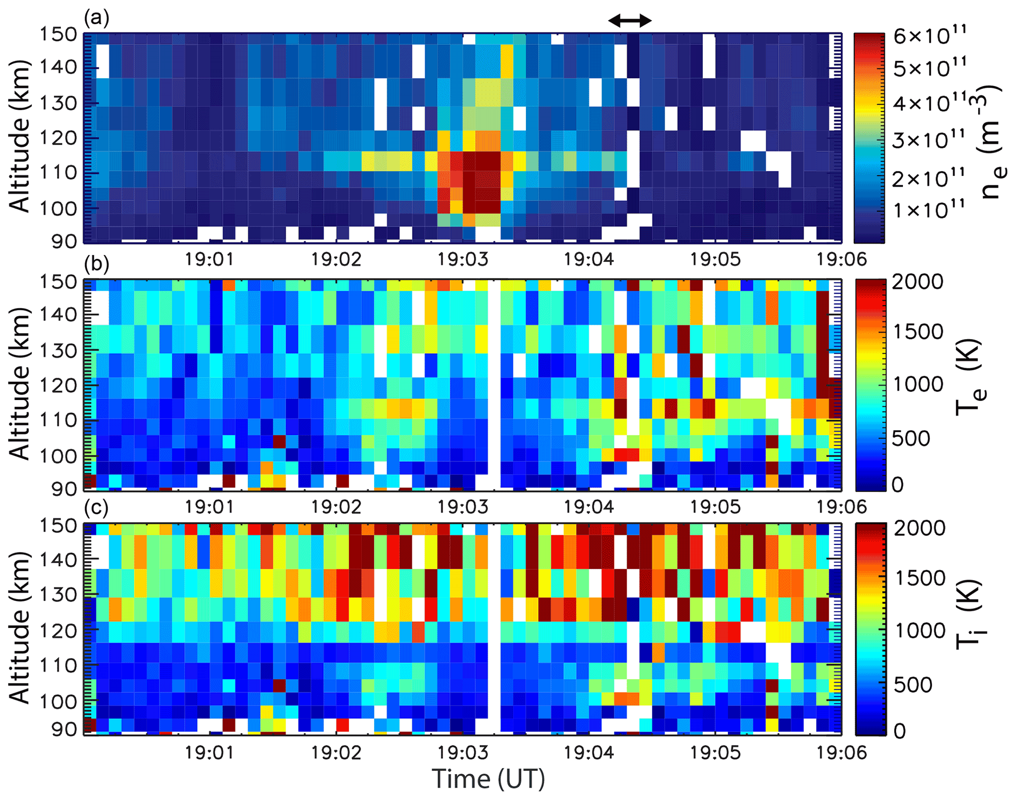
Figure 5 Electron density (a), electron temperature (b), and ion temperature (c) as a function of height and time estimated by ESR during event 1 on 4 December 2013. The time interval of the fragments is indicated by a double-headed arrow on top of panel (a).

The optical data show that the boundary arc is surrounded by fainter auroral emission with less structure. This fainter emission moves out of the radar beam at 19:04:15 UT, which is when the fragments are seen in ASK. The fragments pass near the magnetic zenith but never fill the radar beam. The time interval when they are in the magnetic zenith region of the ASK FOV is marked with a double-headed arrow above the top panel in Fig. 5; there is no signature of them in the radar electron density data. The middle and bottom panels in Fig. 5 show the electron and ion temperature, respectively, in the altitude range from 90 to 150 km. At the time of the fragments, enhancements are seen in both temperatures near 100 km altitude. These temperature increases may indicate that the structures appear in a region of strong electric field adjacent to the boundary arc, where the ion temperature enhancements can be caused by Joule (frictional) heating (e.g. Zhu et al., 2001; Price et al., 2019). Strong electric fields can also drive a non-linear electron Pedersen current, causing intense enhancements of electron temperature localised to a narrow altitude range around 115 km (Saito et al., 2001; Buchert et al., 2008; Schlatter et al., 2013). The electron temperature enhancements could also be caused by Ohmic heating from intense field-aligned currents (Lanchester et al., 2001), although, in that case, they are likely to have a considerable vertical extent along the magnetic field line, which is not clearly present in our observations.

Electron and ion temperature enhancements are also present at 100 km altitude just before 19:05:30 UT. FAEs are again visible in the ASK images at this time, for about 20 s from 19:05:20 UT, although they are dimmer than the FAEs during the main part of the event and fade in and out of visibility, making their sizes and speeds difficult to determine accurately. Again they are poleward of an auroral arc and drift eastward approximately parallel to the arc. FAEs are not present prior to 19:04 UT; they are only visible when the electron and ion temperatures are significantly enhanced at 100 km altitude, providing some evidence that the FAEs themselves occur at this altitude.

SuperDARN (Super Dual Auroral Radar Network) observations indicate that, during both events, Svalbard was located in the dusk sector of the polar cap, but most likely beneath anti-sunward flow across the polar cap, close to the transition to westward flow. Event 1 occurred on the nightside, so the anti-sunward flow is southward, while event 2 occurred on the dayside, so the anti-sunward flow is northward. The convection electric field associated with the anti-sunward flow is, therefore, westward for event 1 and eastward for event 2, which is oppositely directed to the drift of the FAEs. The FAEs reported by Dreyer et al. (2021) also all occurred in the dusk sector of the polar cap close to the flow reversal.

3 Analysis

To constrain theories for the generation mechanism of FAEs, we measure their drift speed and the speed of their internal structure. We term these the group speed and phase speed, respectively, making the assumption that the FAEs are a signature of dispersive waves. We measure the speeds using a keogram, which is a plot formed by taking a cut or slice of pixels from each image in a sequence and then stacking the slices in time order, so that the time is on the abscissa, and the position along the cut is on the ordinate. The movement of the FAEs is approximately parallel to the auroral arc alignment in each event, with a north–south component of their velocity matching the north–south drift of the arc (southwards in event 1; northwards in event 2) to maintain a steady distance between each FAE and the arc. We use a keogram made with a vertical (N–S) cut across the images to determine the velocity of the arc in this direction, and then a keogram with an angled cut, where the cut moves through the images at the same vertical speed as the FAEs (and arc), which allows us to determine the group speed and phase speed of the FAEs in the arc's frame of reference.

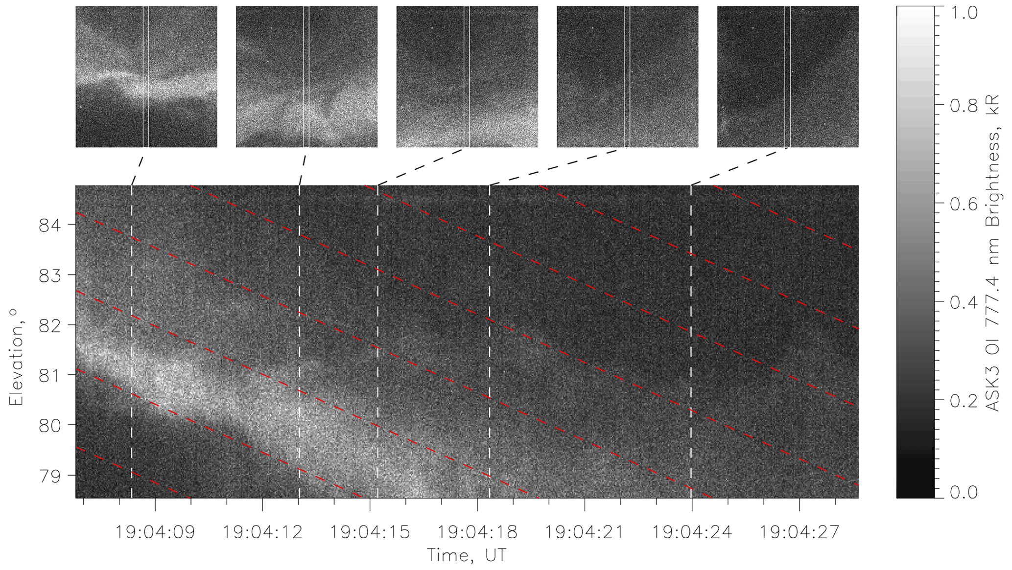
Figure 6 Keogram made using a vertical cut through the centre of the ASK3 (OI 777.4 nm) field of view to show the movement of the auroral arc during event 1. White dashed lines mark the times of the images shown above the keogram. The white boxes indicated in the images show the location of the keogram cut. Red dashed lines indicate the arc motion, with their slope corresponding to the arc's speed in the vertical cut direction.

Figure 6 shows the keogram made using a central N–S cut for event 1. Images in OI 777.4 nm (ASK3) are used to show only the auroral arc and not the FAEs. The cut has a width of 10 pixels and is averaged across this width to improve the signal-to-noise ratio when forming the keogram. Some sample images are shown above the keogram at times corresponding to the white dashed vertical lines drawn over the keogram. The outline of the cut is indicated in white on each sample image. The red dashed lines drawn across the keogram indicate the motion of the arc. The slope of the red dashed lines corresponds to the speed of the arc in the direction of the keogram cut (southwards) and is 0.41 pixels per frame, equivalent to 0.32^∘ s⁻¹.

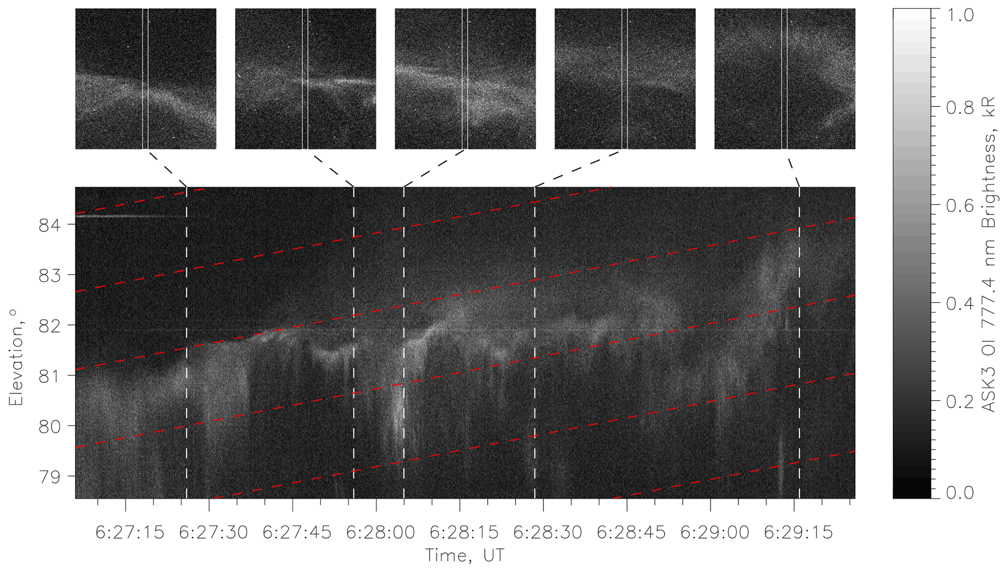
Figure 7 Keogram made using a vertical cut through the centre of the ASK3 (OI 777.4 nm) field of view to show movement of the auroral arc during event 2. White dashed lines mark the times of the images shown above the keogram. The white boxes indicated in the images show the location of the keogram cut. Red dashed lines indicate the arc motion, with their slope corresponding to the arc's speed in the vertical cut direction.

Figure 7 follows the same format as Fig. 6 but shows the N–S cut keogram formed for event 2. The arc in event 2 has a section where it broadens and bends towards the south at around 06:29:00 UT, but overall, the northwards drift is approximately constant and is, again, shown with red dashed lines on the keogram. The emission extending below the arc at 06:28:01–06:28:06 UT is a FAE that is particularly bright in N₂ 1P (673.0 nm, ASK1) and also seen in OI (777.4 nm, ASK3). The northward drift of the arc is found to be 0.045 pixels per frame, which is equivalent to 0.022^∘ s⁻¹.

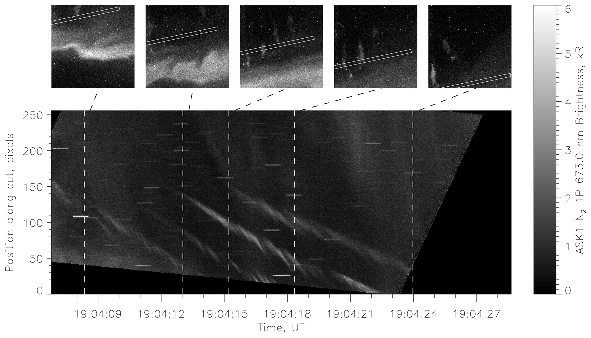
Figure 8 ASK1 (N₂ 1P) keogram made using a moving cut to track the FAEs in event 1. White dashed lines mark the times of the images shown above the keogram. The white boxes indicated in the images show the location of the keogram cut.

The angled cut used to determine the group speed and phase speed of the FAEs is made parallel to the auroral arc, with its velocity perpendicular to its length. The cut is positioned to lie across as many FAEs as possible. The keogram made using such a cut for event 1 is shown in Fig. 8 in the same format as in Figs. 6 and 7. The location of the cut is outlined in white in the images above the keogram. This time the N₂ 1P (ASK1) emission is shown so that the keogram displays the motion of the FAEs. Each FAE is clearly made up of repeating internal structures moving faster than the FAE, i.e. the phase speed is greater than the group speed. The FAEs and their internal structures were manually traced by drawing straight lines on top of the keogram. The slope of these lines was then used to determine the group speed and phase speed.

Figure 9 ASK1 (N₂ 1P) keogram made using a moving cut to track the FAEs in event 2a. White dashed lines mark the times of the images shown above the keogram. The white boxes indicated in the images show the location of the keogram cut.

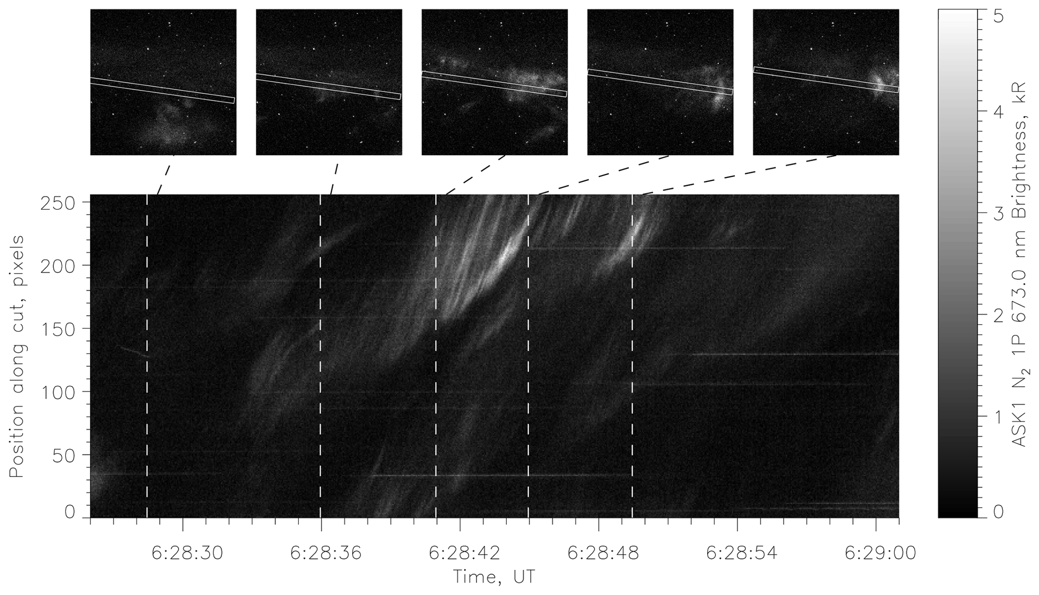
Figure 10 ASK1 (N₂ 1P) keogram made using a moving cut to track the FAEs in event 2b. White dashed lines mark the times of the images shown above the keogram. The white boxes indicated in the images show the location of the keogram cut.

Event 2 was analysed in the same way as event 1, but since it is considerably longer, two portions were selected to determine the group speed and phase speed, which we refer to as event 2a (shown in Fig. 9) and event 2b (shown in Fig. 10). The motion of the keogram cut is continuous from event 2a to event 2b.

Table 1 Mean group speeds and mean phase speeds of the FAEs within each event. The uncertainties given here are the standard deviations across all measurements within the event.

The group and phase speeds determined from the keograms for the two events are shown in Table 1 and are all for an assumed altitude of 100 km. The speeds obtained from a combination of measurements from events 2a and 2b are also given.

4 Discussion and theory

Despite the morphological differences between the FAEs in event 1 and event 2, the similarities in internal dynamics and velocities suggest a common generation mechanism. Here we use our results to constrain theories for what that generation mechanism might be.

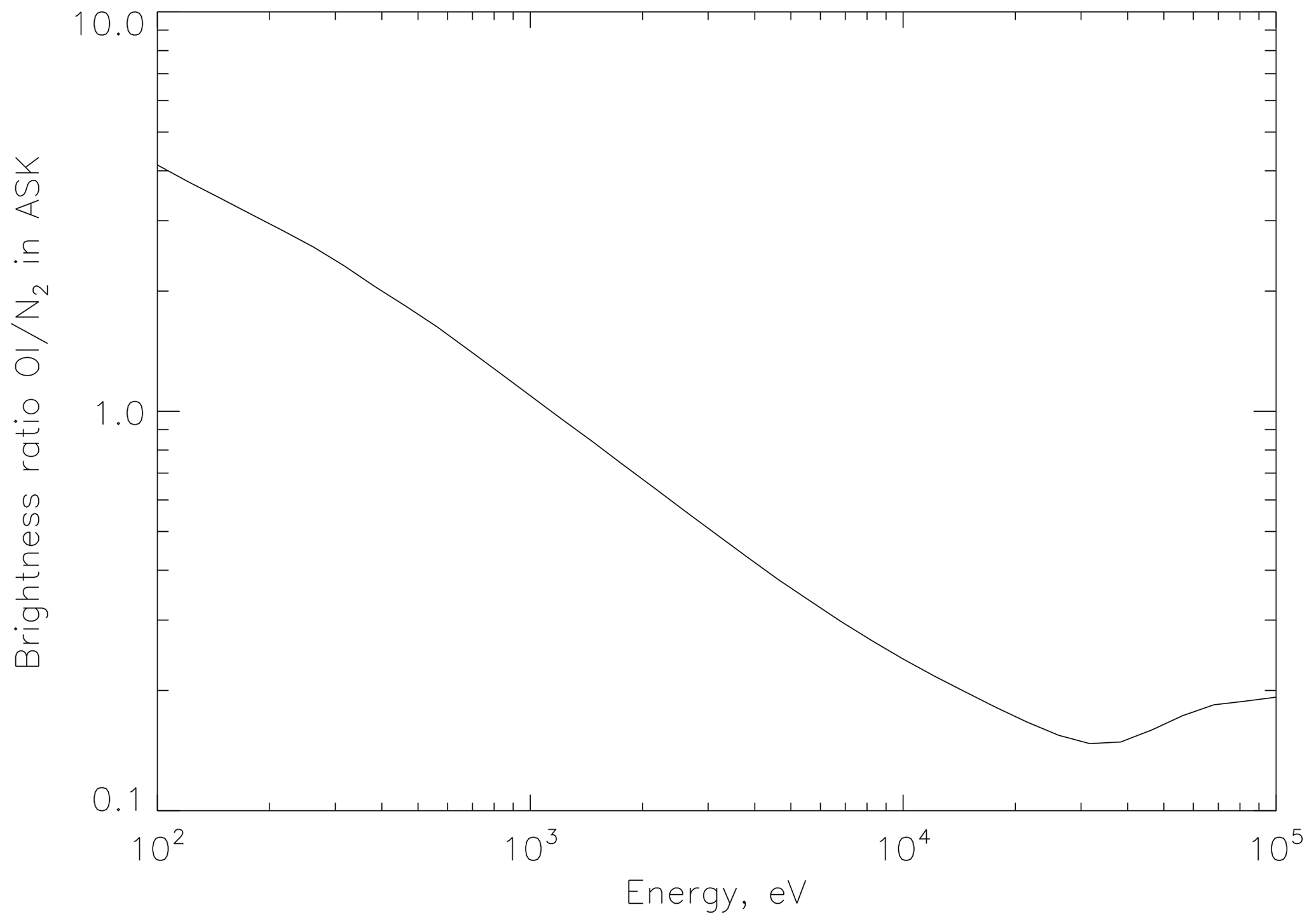
Figure 11 Modelled auroral OI $/$ N₂ brightness ratio for electron precipitation, from 10 eV to 100 keV, for conditions during event 1. The emissions are calculated through the ASK filters so that ASK observations can be directly compared with the model results.

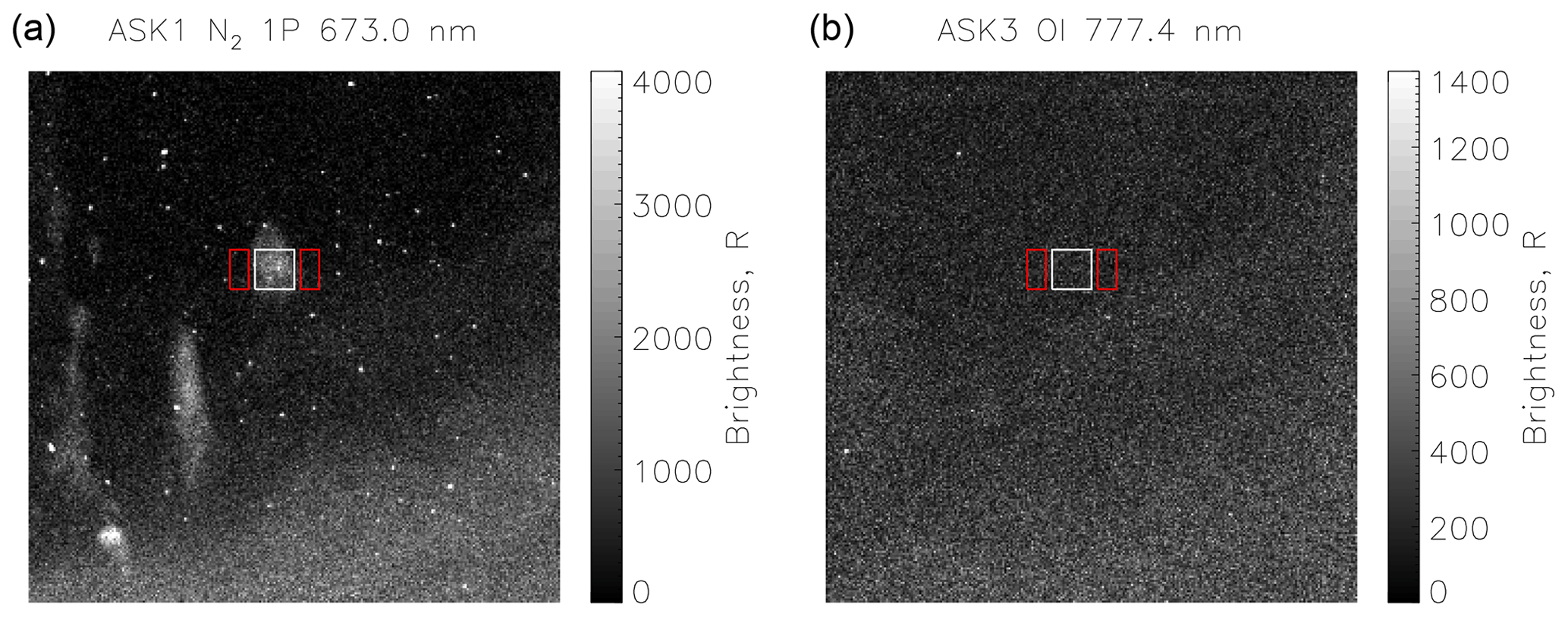
Figure 12 Simultaneous images in N₂ 1P (a; ASK1) and OI 777.4 nm (b; ASK3) at 19:04:19.063 UT during event 1. The region used to calculate the brightness of a selected FAE is shown with a white box, and the regions used to calculate the background intensity are shown with red boxes.

If the FAEs were a result of auroral electron precipitation, then they would be observed in the OI 777.4 nm emission and in the N₂ 1P emission. The OI 777.4 nm emission is a result of two excitation processes, i.e. direct excitation of O (from predominantly low-energy primary precipitation) and dissociative excitation of O₂ (from predominantly high-energy precipitation). ASK exploits this fact to routinely estimate the energy and flux of precipitation by measuring the ratio of brightness of the OI (777.4 nm) and N₂ 1P (673.0 nm) emissions (e.g. Lanchester et al., 2009; Lanchester and Gustavsson, 2012; Whiter et al., 2010; Dahlgren et al., 2011). The relationship between the OI $/$ N₂ brightness ratio and electron precipitation energy is determined using the Southampton ionospheric model (Lanchester et al., 2009), which combines time-dependent electron transport (Lummerzheim and Lilensten, 1994) with ion chemistry (see the Appendix in Lanchester et al., 2001). Model results for conditions during event 1 (date, time, F10.7, 81 d average F10.7, and Ap index are used as inputs to the MSISE-90 model (Hedin, 1991) to provide densities of the major neutral species) are plotted in Fig. 11; the modelled emission brightness is calculated through the ASK filters to allow direct comparison with observations. We have determined the brightness ratio in a selected FAE in event 1 which is reasonably bright in N₂ 1P, without significantly overlapping the adjacent auroral arc, from the images shown in Fig. 12. The brightness of the FAE is calculated as the median pixel intensity in a 20×20 pixel box containing the FAE (drawn in white) with a background value similarly calculated from two 10×20 pixel boxes either side of the FAE (red). The brightness of the FAE in N₂ 1P (673.0 nm) is 1142±35.4 R, and in OI (777.4 nm) is 40.2±8.2 R, giving an OI $/$ N₂ ratio of 0.035±0.007. The model results show that such a low brightness ratio cannot be caused by auroral precipitation. Even for high-energy precipitation (10 s of kiloelectron volts), the OI 777.4 nm emission has a brightness of at least 10 % of the N₂ 1P emission through the molecular component of the emission. Therefore, we exclude the possibility that the FAEs are a signature of precipitation modulated by some process above the E-region ionosphere and conclude that the generation mechanism is local to the FAEs.

A morphological argument, similar to that made by Semeter et al. (2020) for streaks, provides secondary evidence for this conclusion; if the FAEs were caused by precipitation, then the field-aligned extent of the emission region should result in the shape elements converging towards the magnetic zenith, which is not the case even when the FAEs are located at the edge of the ASK field of view away from magnetic zenith. It should be noted that high-energy precipitation can result in thin emission layers barely exhibiting any perspective effect (e.g. Ivchenko et al., 2005); however, even in the case of monoenergetic high-energy precipitation, locally excited atomic oxygen emissions are observed co-located with the molecular emission in the thin layer (Dahlgren et al., 2012), which is not the case for the FAEs.

The excitation thresholds for the N₂ 1P and OI emissions observed by ASK provide information on the energy of ionospheric electrons presumed to be responsible for exciting the FAEs. The ASK1 camera observes emission from the (5,2) and (4,1) vibrational bands of N₂ 1P, which contains transitions from the B³Π_g state to the A${}^{\mathrm{3}}{\mathrm{\Sigma }}_{\mathrm{u}}^{+}$ state of N₂. The upper state has an excitation threshold of 7.353 eV (Itikawa, 2005), although in aurora the upper state is fed by cascading from higher states, so the effective excitation threshold for auroral emission is about 8.5 eV (Ashrafi et al., 2009). Cascading may play a smaller role in FAEs than in normal aurora, but in any case, the excitation threshold for the N₂ emission observed by ASK is about 7–8 eV and is greater than the excitation threshold for the OI 557.7 nm emission which, therefore, must give the green colour seen in the all-sky camera images. The OI 777.4 nm emission has excitation thresholds of 15.9 eV for the dissociative contribution (Erdman and Zipf, 1987) and 10.76 eV for the direct excitation contribution. For almost all FAEs in event 1, the 777.4 nm emission is either completely absent or extremely weak, giving an upper limit to the electron energy of 10.76 eV. Some bright FAEs in event 2, and the brightest two FAEs at the end of event 1, do show emission in 777.4 nm, so the upper limit for those FAEs must be greater than 10.76 eV. The cross section for the direct excitation to the upper state of the 777.4 nm emission (O⁵P) is strongly peaked just above the threshold (Lanchester et al., 2009; Julienne and Davis, 1976), and therefore, the turning on of 777.4 nm emission does not necessarily signify a significant increase in energy.

An electron temperature greater than about 2300 K is required to thermally excite significant OI 630.0 nm emission (Carlson et al., 2013; Kwagala et al., 2017), which has a much lower excitation threshold (1.96 eV) than the emission observed by ASK. The electron temperature during event 1 was below 2000 K, and therefore, there cannot be any significant thermally excited emission, suggesting the presence of a non-thermal (i.e. accelerated) electron population which excites the N₂ 1P emission.

4.1 Electrostatic ion cyclotron waves

Based on their morphology and appearance, we make the assumption that the FAEs are generated by some sort of wave or instability which accelerates ionospheric electrons. The ASK observations show that the wave propagates perpendicular (or nearly perpendicular) to the magnetic field, and the group speed and phase speed of the FAEs are approximately half and double the ion acoustic speed, respectively, which is consistent with the properties of electrostatic ion cyclotron (EIC) waves. If we assume the FAEs are located at the altitude of the enhanced electron and ion temperatures (T_e and T_i, respectively) seen in the ESR data (100 km), we can use the temperature measurements to estimate the ion acoustic speed at the FAEs as follows:

$$\begin{array}{}\text{(1)}& c_{\mathrm{s}}=\sqrt{{\displaystyle \frac{{\mathit{\gamma }}_{\mathrm{e}}{k}_{\mathrm{B}}{T}_{\mathrm{e}}Z+{\mathit{\gamma }}_{\mathrm{i}}{k}_{\mathrm{B}}{T}_{\mathrm{i}}}{M_{\mathrm{i}}}}},\end{array}$$

where Z is the ion charge, M_i is the ion mass, k_B is the Boltzmann constant, and γ_e and γ_i are the heat capacity ratios for electrons and ions, respectively. Using T_e=1800 K and T_i=1600 K (both from ESR), and γ_e=1 and γ_i=3 (for ion plasma waves), gives an ion acoustic speed c_s=1352 m s⁻¹ for NO⁺ ions. The dispersion relation for EIC waves is commonly given as follows:

$$\begin{array}{}\text{(2)}& {\mathit{\omega }}^{\mathrm{2}}={\mathrm{\Omega }}_{\mathrm{i}}^{\mathrm{2}}+k^{\mathrm{2}}{c}_{\mathrm{s}}^{\mathrm{2}},\end{array}$$

where ω is the wave frequency, Ω_i is the ion cyclotron frequency, and k is the wavenumber. From the dispersion relation, we find that the group velocity (v_g) and phase velocity (v_p) are related by $v_{\mathrm{g}}{v}_{\mathrm{p}}=c_{\mathrm{s}}^{\mathrm{2}}$, which is satisfied by our observations and estimate of c_s.

The wavelength of the FAE internal structure appears to be of the order of 10–20 pixels, corresponding to 425–850 m at 100 km altitude, although the distance between consecutive phase fronts (internal structures) varies from front to front. Combined with the measured phase speed for event 1, this wavelength gives a wave frequency of about 18–36 s⁻¹. This frequency is considerably lower than the ion cyclotron frequency in the E-region ionosphere; even Fe⁺ (which may be present in a sporadic E layer) has a cyclotron frequency of 90 s⁻¹. The apparent wavelength is, therefore, not consistent with the EIC dispersion relation given above. One possibility is that not all phase fronts are visible in the keograms, which could be caused by the keogram cut crossing different phases across its width. The fact that the distance between internal structures varies could also be because only certain phase fronts are optically visible for some reason. Perhaps a more likely explanation is that the EIC dispersion relation does not accurately describe the FAEs, either because EIC waves are not the generation mechanism or because the standard dispersion relation is not valid.

Coherent radar echoes of the sort known as type 3 echoes have previously been attributed to NO⁺ EIC waves in the E-region ionosphere (e.g. D'Angelo, 1973; Fejer et al., 1984; Prikryl et al., 1987). However, it was thought that the echoes originated at altitudes above about 140 km where the ions are magnetised, i.e. the ion-neutral collision frequency ν_i<Ω_i. Once the altitude of the type 3 irregularities was shown by Sahr et al. (1991) to be at lower altitudes of 100–120 km, the EIC wave explanation was largely discounted on the basis that there is no cyclotron motion of the ions. If our assumption that FAEs are located at about 100 km altitude is correct, we could similarly conclude that they cannot be a signature of EIC waves. However, if the FAEs were located above 140 km, where EIC waves are possible, our measured speeds should be multiplied by at least 1.4 and, to be consistent with the EIC dispersion relation, our estimate of c_s must be increased by the same factor. Higher ion and electron temperatures (e.g. $T_{\mathrm{e}}\sim T_{\mathrm{i}}\sim$3000 K) or a change from NO⁺ to O⁺ ions could provide the required increase.

4.2 Farley–Buneman instability

Dreyer et al. (2021) suggested that FAEs may be caused by the Farley–Buneman instability, for which the dispersion relation is commonly given as follows:

$$\begin{array}{}\text{(3)}& \mathit{\omega }={\displaystyle \frac{k{v}_{\mathrm{d}}}{\mathrm{1}+\mathit{\psi }}},\end{array}$$

where v_d is the E×B drift speed, and ψ is given by the following:

$$\begin{array}{}\text{(4)}& \mathit{\psi }={\displaystyle \frac{{\mathit{\nu }}_{\mathrm{e}}{\mathit{\nu }}_{\mathrm{i}}}{{\mathrm{\Omega }}_{\mathrm{e}}{\mathrm{\Omega }}_{\mathrm{i}}}},\end{array}$$

where ν_e and ν_i are the electron-neutral and ion-neutral collision frequencies, and Ω_e is the electron cyclotron frequency. With this dispersion relation, the phase velocity and group velocity of the instability are equal, and therefore, it does not match our observations, unless the interpretation of the motion of the FAEs and their internal structure as group and phase velocity of a wave or instability is incorrect.

Litt et al. (2015) derived a modified dispersion relation for the Farley–Buneman instability which incorporates the effects of ion thermal motion as follows:

$$\begin{array}{}\text{(5)}& \mathit{\omega }={\displaystyle \frac{\mathit{k}.{\mathit{v}}_{\mathrm{d}}}{(\mathrm{1}+\mathit{\psi })}}-{\displaystyle \frac{{\mathit{\nu }}_{\mathrm{e}}}{{\mathit{\nu }}_{\mathrm{i}}}}{\displaystyle \frac{v_{\mathrm{Ti}}^{\mathrm{2}}{k}^{\mathrm{2}}}{{\mathrm{\Omega }}_{\mathrm{e}}{\mathrm{\Omega }}_{\mathrm{i}}}}{\displaystyle \frac{\mathit{k}.{\mathit{v}}_{\mathrm{d}}}{(\mathrm{1}+\mathit{\psi }{)}^{\mathrm{2}}}},\end{array}$$

where v_Ti is the ion thermal speed, and other symbols are as defined above. In this case, we derive a relationship between the group and phase speed as follows:

$$\begin{array}{}\text{(6)}& v_{\mathrm{g}}=\mathrm{3}{v}_{\mathrm{p}}-{\displaystyle \frac{\mathrm{2}{v}_{\mathrm{d}}}{\mathrm{1}+\mathit{\psi }}},\end{array}$$

with the assumption that k and v_d are parallel. Using estimates of neutral density at 100 km altitude during event 1 from the MSISE-90 model (Hedin, 1991) and the electron temperature measured by ESR, together with coefficients given by Schunk and Nagy (2000), we obtain estimates for the electron-neutral collision frequency ${\mathit{\nu }}_{\mathrm{e}}=\mathrm{3.44}\times {\mathrm{10}}^{\mathrm{5}}$ s⁻¹ and ion-neutral collision frequency for NO⁺ ions ${\mathit{\nu }}_{\mathrm{i}}=\mathrm{4.98}\times {\mathrm{10}}^{\mathrm{3}}$ s⁻¹. The cyclotron frequencies for electrons and NO⁺ ions at 100 km altitude above Svalbard, where the total magnetic field magnitude is approximately 52 570 nT, are ${\mathrm{\Omega }}_{\mathrm{e}}=\mathrm{9.25}\times {\mathrm{10}}^{\mathrm{6}}$ s⁻¹ and Ω_i=168 s⁻¹. With these values, we calculate ψ=1.11 and then, using the measured group and phase speeds from event 1, obtain an E×B drift speed v_d=6940 m s⁻¹, which corresponds to an electric field magnitude of 365 mV m⁻¹. Although this drift speed is very high, such an electric field is possible in a localised region next to an auroral arc (e.g. Lanchester et al., 1996; Tuttle et al., 2020; Marklund et al., 1994).

Previous work on electron and ion heating suggests that such a large electric field would produce temperatures much higher than those measured by ESR during event 1 (e.g. Bahcivan, 2006), but the spatial and temporal averaging required to measure electric fields using radar leads to an underestimate of the peak electric field value (Tuttle et al., 2020; Codrescu et al., 1995); a highly localised E-field magnitude of 300–400 mV m⁻¹ may not be inconsistent with an observed electron temperature of about 2000 K. Farley–Buneman waves could be responsible for the electron heating through non-precipitation electron-neutral collisions (Saito et al., 2001), which may also produce the FAEs we observe through excitation of vibrational and rotational modes of N₂.

Auroral arcs have an electric field associated with them which is perpendicular to the arc's length and points towards the arc on either side (Opgenoorth et al., 1990; Aikio et al., 1993; Lanchester et al., 1996). The combination of the arc-associated electric field and background convection electric field can lead to an asymmetric total electric field, such that it is stronger on one side of the arc than the other. Price et al. (2019) found significant differences in Joule heating on the two sides of an arc, with a hotter neutral temperature on the poleward side of the arc in the morning sector. If the electric field on either side of an arc is different (in magnitude, direction, or both), so that the E×B drift speed is also different, then we would expect the properties of FAEs on either side of the arc to vary in order to satisfy Eq. (6). High-resolution observations of FAEs crossing an arc, or appearing on both sides of an arc, would, therefore, provide an opportunity to further examine whether the FAEs could be caused by the Farley–Buneman instability. We note that, as the last FAE in event 1 left the ASK field of view, it appeared to tilt so as to stay perpendicular to the arc, which may be an indication that the FAEs are aligned with the arc-associated electric field.

Robinson and Honary (1993) found that the ratio between the phase speed of a Farley–Buneman wave and the ion acoustic speed, $v_{\mathrm{p}}/c_{\mathrm{s}}$, is between 1 and $\sqrt{\mathrm{5}/\mathrm{3}}$, which would suggest a minimum ion acoustic speed during our events of about 1700 m s⁻¹. Although fast, this speed may be consistent with the O⁺ ion acoustic speed in the region of enhanced temperatures (see Sect. 4.1). However, Robinson and Honary (1993) did not consider E×B drift velocities larger than 2400 m s⁻¹, which makes it problematic to directly compare their results with our observations.

4.3 Further considerations

Besides matching the observations described in this work, theories for the generation mechanism of the FAEs must also explain why the FAEs are rare and only visible at some times. Currently, the number of observations of FAEs is limited, which makes it difficult to determine what conditions are necessary for their formation. One common feature of our event 1 and the FAEs reported by Dreyer et al. (2021) is the high ion and electron temperatures seen at a low altitude (<110 km) in the radar measurements. However, high temperatures can be measured without the appearance of FAEs (e.g. Price et al., 2019), so this is clearly not the only requirement for their occurrence, although the mechanism producing FAEs may also produce high temperatures. If the FAEs are produced by the Farley–Buneman instability, then both of our events must have occurred in regions of strong E fields of a few hundred millivolts per metre (mV m⁻¹), which may be a requirement for their occurrence. We note that all known observations of FAEs have occurred in the evening sector of the polar cap close to the flow reversal, but given the limited number of observations, it is not yet certain that this is a favoured location for their formation. All observations have been reported from the same geographic location on Svalbard, which will bias statistics on the location of FAEs within the global convection pattern.

Our calculations and discussion rely on several assumptions, such as that the altitude of the FAEs corresponds to the enhanced temperatures measured by ESR. We also assume that the FAEs move at the group speed of a wave, with the internal structure moving at the phase speed, based on the appearance of the FAEs in our keograms. This assumption is a substantial one, and we note that our attempt to explain the observations in terms of simplified linear theory concepts may have limited applicability, especially given the non-linear nature of low altitude electron heating by strong E fields (Buchert et al., 2008).

The observations at least partially match the properties of the Farley–Buneman instability and, alternatively, of EIC waves, but further observations and analysis are required to confirm or exclude either of these waves as the generation mechanism for the FAEs. In particular, it would be advantageous to measure the altitude of the FAEs and to observe FAEs on both sides of an auroral arc.

5 Conclusions

High-resolution imaging of fragments of aurora-like emission during two separate events has revealed FAE drift speeds of 580–700 m s⁻¹, with internal dynamics moving at speeds of 2200–2500 m s⁻¹. The appearance of the FAEs suggests that these speeds may correspond to the group speed and phase speed, respectively, of the instability producing the FAEs, although this conclusion is not certain. While these speeds satisfy the dispersion relation for electrostatic ion cyclotron waves, their apparent wavelength corresponds to a wave frequency below the NO⁺ ion cyclotron frequency, and the assumed altitude of the FAEs is inconsistent with EIC waves. The observed speeds also match the dispersion relation for the Farley–Buneman instability derived by Litt et al. (2015), for an E×B drift speed of about 7 km s⁻¹, corresponding to a perpendicular electric field of 365 mV m⁻¹. Although extreme, these values are possible close to auroral arcs and might be sufficient to produce the FAEs. We emphasise that these conclusions are subject to several caveats and assumptions, in particular that the location of the FAEs corresponds to a region of enhanced electron temperature at 100 km altitude. If the FAEs are at higher or lower altitude, the measured speeds must be scaled accordingly.

Any theory for the generation mechanism of FAEs should explain why they are not more commonly observed. However, advances in imaging technology have made it easier to detect the FAEs, so they may be found to be quite common at high latitude. Further observations will undoubtedly help to explain the physics of FAEs. Aurora Zoo has highlighted one of the strengths of citizen science in identifying unusual events. As more ASK observations are added to Aurora Zoo, we are optimistic that more FAE events will be found.