Seasonal features of geomagnetic activity: a study on the solar activity dependence

Seasonal features of geomagnetic activity and their solar-wind–interplanetary drivers are studied using more than five solar cycles of geomagnetic activity and solar wind observations. This study involves a total of 1296 geomagnetic storms of varying intensity identified using the Dst index from January 1963 to December 2019, a total of 75 863 substorms identified from the SuperMAG AL/SML index from January 1976 to December 2019 and a total of 145 high-intensity long-duration continuous auroral electrojet (AE) activity (HILDCAA) events identified using the AE index from January 1975 to December 2017. The occurrence rates of the substorms and geomagnetic storms, including moderate ($-\mathrm{50}\mathrm{nT}\ge \text{Dst}>-\mathrm{100}\mathrm{nT}$) and intense ($-\mathrm{100}\mathrm{nT}\ge \text{Dst}>-\mathrm{250}\mathrm{nT}$) storms, exhibit a significant semi-annual variation (periodicity ∼6 months), while the super storms ($\text{Dst}\le -\mathrm{250}$ nT) and HILDCAAs do not exhibit any clear seasonal feature. The geomagnetic activity indices Dst and ap exhibit a semi-annual variation, while AE exhibits an annual variation (periodicity ∼1 year). The annual and semi-annual variations are attributed to the annual variation of the solar wind speed V_sw and the semi-annual variation of the coupling function VB_s (where V = V_sw, and B_s is the southward component of the interplanetary magnetic field), respectively. We present a detailed analysis of the annual and semi-annual variations and their dependencies on the solar activity cycles separated as the odd, even, weak and strong solar cycles.

1 Introduction

Solar-wind–magnetosphere energy coupling causes disturbances in the magnetosphere of the Earth (e.g., Dungey, 1961; Axford and Hines, 1961; Tsurutani et al., 1992; Gonzalez et al., 1994; Tsurutani et al., 2020). Depending on the strength, duration and efficiency of the coupling, resultant geomagnetic disturbances (von Humboldt, 1808) can be classified as magnetic storms, substorms and high-intensity long-duration continuous auroral electrojet (AE) activities (HILDCAAs) (see Gonzalez et al., 1994; Hajra et al., 2020; Hajra, 2021a). In general, magnetic storms represent global-scale disturbances caused by enhancements in (westward) ring current flowing at ∼2–7 Earth radii (R_Earth) in the magnetic equatorial plane of the Earth (Gonzalez et al., 1994; Lakhina and Tsurutani, 2018, and references therein). Storm duration spans a few hours to several days. In fact, while the storm main phase lasts typically for ∼10–15 h, the recovery phase can continue much longer, from hours to several days (Gonzalez et al., 1994). Substorms (Akasofu, 1964) are shorter-scale, a few minutes to a few hours, disturbances in the nightside magnetosphere (magnetotail) resulting in precipitations of ∼10–100 keV electrons and protons in the auroral ionosphere (e.g., Meng et al., 1979; Thorne et al., 2010; Tsurutani et al., 2019, and references therein). Intense auroral substorms continuing for a few days without occurrence of any major magnetic storms have been called HILDCAAs (Tsurutani and Gonzalez, 1987; Hajra et al., 2013) to distinguish them from nominal substorms and major magnetic storms (Tsurutani et al., 2004; Guarnieri, 2006).

It is important to note that from the physical point of view, substorms and HILDCAAs are two different types of geomagnetic activity. While substorms may occur during HILDCAAs, they represent different magnetosphere/ionosphere processes (Tsurutani et al., 2004; Guarnieri, 2005, 2006). For example, HILDCAAs are associated with Alfvén wave trains carried by solar wind high-speed (∼550–850 km s⁻¹) streams (HSSs) emanated from solar coronal holes (Tsurutani and Gonzalez, 1987; Hajra et al., 2013). The intermittent magnetic reconnection between the Alfvén wave southward component and geomagnetic field results in intermittent increases in auroral activity during HILDCAAs. Substorms, on the other hand, are associated with solar wind energy loading in the magnetotail caused by magnetic reconnection (Tsurutani and Meng, 1972), and subsequent explosive release of the energy in the form of energetic particles and strong plasma flows (e.g., Akasofu, 1964, 2017; Rostoker, 2002; Nykyri et al., 2019, and references therein). These are not essentially associated with HSSs. Thus, for good reason, the term “substorm” was avoided in the definition of HILDCAAs by Tsurutani and Gonzalez (1987). Later, Hajra et al. (2014b, 2015a, b) have shown that HILDCAAs take an important role in the acceleration of relativistic (∼ MeV) electrons in the outer radiation belt of the Earth. This feature further distinguishes the HILDCAAs from nominal substorms.

Geomagnetic activity, in general, is known to be highly variable, modulated by several solar–terrestrial features. The solar/interplanetary sources of the variability include the ∼27 d solar rotation (Bartels, 1932, 1934; Newton and Nunn, 1951), the ∼11-year solar activity cycle (Schwabe, 1844), the electromagnetic and corpuscular radiations from the Sun, several plasma emission phenomena, heliospheric current region, etc. On the other hand, the Earth's translational movement (solstices), the inter-hemispheric symmetry (equinoxes), and the observational frame of reference or the coordinate system (Russell, 1971) can also largely impact the geomagnetic activity variation.

One of the earliest reported features of the geomagnetic activity is the semi-annual variation, that is, more frequent occurrences and higher strength during equinoxes and lesser occurrences and weaker strength during solstices (e.g., Broun, 1848; Sabine, 1852). The semi-annual variation is reported in the occurrence rates and intensities of the magnetic storms (e.g., Cliver et al., 2000, 2004; Le Mouël et al., 2004; Cnossen and Richmond, 2012; Danilov et al., 2013; McPherron and Chu, 2018; Lockwood et al., 2020) and in the Earth's radiation belt electron variations (e.g., Baker et al., 1999; Li et al., 2001; Kanekal et al., 2010; Katsavrias et al., 2021). This is generally explained in the context of the Earth's position in the heliosphere (known as the “axial effect”; Cortie, 1912), relative angle of solar wind incidence with respect to Earth's rotation axis (the “equinoctial effect”; Boller and Stolov, 1970) and geometrical controls of interplanetary magnetic fields (the “Russell–McPherron effect”; Russell and McPherron, 1973). See Lockwood et al. (2020) for an excellent discussion of the mechanisms. While both the equinoctial and the Russell–McPherron effects are shown to be responsible for the semi-annual variation in the geomagnetic indices (e.g., Cliver et al., 2000; O'Brien and McPherron, 2002), the semi-annual variation in the relativistic electron fluxes of the outer belt is mainly attributed to the Russell–McPherron effect (e.g., Kanekal et al., 2010; Katsavrias et al., 2021).

However, the semi-annual variation in general was questioned by the work of Mursula et al. (2011) reporting solstice maxima in substorm frequency and duration, as well as substorm amplitude and global geomagnetic activity peaks alternating between spring and fall in ∼11 years. While solstice maxima were attributed to auroral ionospheric conductivity changes (Wang and Lühr, 2007; Tanskanen et al., 2011), the alternating equinoctial maxima were associated with asymmetric solar wind distribution in solar hemispheres (Mursula and Zieger, 2001; Mursula et al., 2002). In addition, several recent studies have reported a lack of any seasonal dependence for substorms (Hajra et al., 2016), HILDCAAs (Hajra et al., 2013, 2014a) or in the radiation belts (Hajra, 2021b).

In the present work, for the first time, we will explore a long-term database of substorms, HILDCAAs, and magnetic storms of varying intensity along with different geomagnetic indices to study the seasonal features of geomagnetic disturbances. The main aim is to identify and characterize the seasonal features of geomagnetic disturbances of different types and intensities. In addition, we will study their solar activity dependencies, if any.

2 Database and methods

Details of the geomagnetic events studied in this work are summarized in Table 1. Auroral substorms are identified by intensification in the auroral ionospheric (westward) electrojet currents. In the present work, we will use the substorm list available at the SuperMAG website (https://supermag.jhuapl.edu/, last access: 23 May 2021; Newell and Gjerloev, 2011; Gjerloev, 2012). The substorm expansion phase onsets were identified from the SML index which is the SuperMAG equivalent of the westward auroral electrojet index AL (see the cited references for details). The present work involves a total of 75 863 substorms identified from January 1976 to December 2019 (Table 1).

Hajra et al. (2021)Hajra et al. (2021)

Table 1 Details of the geomagnetic activity events under present study.

We will use the geomagnetic storm and HILDCAA database prepared by Hajra et al. (2021) for the present work. It is an updated version of the lists presented in Echer et al. (2011), Hajra et al. (2013) and Rawat et al. (2018). Geomagnetic storm onset, main phase, peak strength, recovery phase and storm end are determined by the variations of the Dst index (Sugiura, 1964). Based on the Gonzalez et al. (1994) definition, intervals with the Dst minimum $\le -\mathrm{50}$ nT are identified as magnetic storms. From January 1963 to December 2019, 1296 magnetic storms were identified (Table 1). Geomagnetic storms with the Dst minimum values between −50 nT and −100 nT are classified as the “moderate storms”, between −100 nT and −250 nT as the “intense storms”, and those with the Dst minima lower than −250 nT as the “super storms”. Among all storms studied here, 75 % are moderate, 23 % are intense and only 2 % are super storms.

The HILDCAA events are identified based on four criteria suggested by Tsurutani and Gonzalez (1987). The criteria are (1) the AE index should reach an intensity equal to or greater than 1000 nT at some point during the event (the high-intensity criterion), (2) the event must last at least 2 d (the long-duration criterion), (3) the AE index should not fall below 200 nT for more than 2 h at a time (the continuity criterion), and (4) the auroral activity must occur outside the main phase of a geomagnetic storm or during a non-storm condition ($\text{Dst}>-\mathrm{50}$ nT). Present work involves a total of 145 HILDCAA events identified during January 1975 through to December 2017 (Table 1).

The geomagnetic indices, namely, the ring current index Dst, the global-scale geomagnetic activity index ap and the auroral ionospheric current-related index AE, are used to provide a quantitative measure of the activity level of the terrestrial magnetosphere (Rostoker, 1972). In addition, solar wind parameters are used to study the energy dissipation in the magnetosphere. The D₅₀₀ parameter is defined as the percentage of days with the peak solar wind speed V_sw equal or higher than 500 km s⁻¹ in each month of a year. We estimated the solar wind electric field VB_s, which is an important solar-wind–magnetosphere coupling function (Burton et al., 1975; Tsurutani et al., 1992; Finch et al., 2008). As VB_s involves both the solar wind velocity V_sw (for V) and the southward component of the interplanetary magnetic field (IMF) B_s, the latter being important for magnetic reconnection, VB_s is also called the reconnection electric field. The Akasofu ϵ coupling function (Perreault and Akasofu, 1978), expressed as $V_{\text{sw}}{B}_{\mathrm{0}}^{\mathrm{2}}{\sin }^{\mathrm{4}}(\mathit{\theta }/\mathrm{2})R_{\text{CF}}^{\mathrm{2}}$, was also estimated in this work as a proxy for the magnetospheric energy input rate. Here B₀ represents the magnitude of the IMF, θ is the IMF orientation clock angle and R_CF is the Chapman–Ferraro magnetopause distance (Chapman and Ferraro, 1931).

Table 2 Details of the solar cycles under present study.

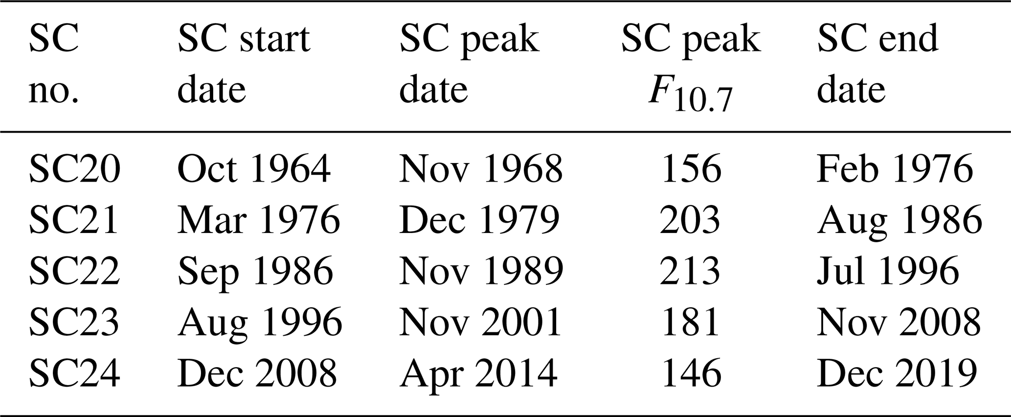
The 10.7 cm solar flux (F_10.7) is shown to be a good indicator of the solar activity (e.g., Tapping, 1987). Thus, the ∼11-year solar cycles (Schwabe, 1844) are studied using the monthly mean F_10.7 solar flux variation. The starting, peak and end dates along with the peak F_10.7 flux of each solar cycle (SC) are listed in Table 2. The F_10.7 fluxes are given in the solar flux unit (sfu), where $\mathrm{1}\mathrm{sfu}={\mathrm{10}}^{-\mathrm{22}}$ $\mathrm{W}{\mathrm{m}}^{-\mathrm{2}}{\mathrm{Hz}}^{-\mathrm{1}}$. Based on the F_10.7 peaks, cycles SC20 and SC24 can be classified as the “weak cycles” (average F_10.7 peak ∼151 sfu) and SC19, SC21, SC22 and SC23 as the “strong cycles” (average F_10.7 peak ∼207 sfu). It can be mentioned that SC24 is the weakest cycle in the space exploration era (after 1957). A detailed study on the solar and geomagnetic characteristics of this cycle is presented in Hajra (2021c). The solar cycles are also grouped into the “even” (SC20, SC22, SC24) and the “odd” (SC19, SC21, SC23) cycles in this work. Previous studies have reported significant differences between the even and odd cycle amplitudes (e.g., Waldmeier, 1934; Gnevyshev and Ohl, 1948; Wilson, 1988; Durney, 2000), and in their geomagnetic responses (e.g., Hajra et al., 2021; Owens et al., 2021).

We will apply the Lomb–Scargle periodogram analysis (Lomb, 1976; Scargle, 1982) to identify the significant periodicities in the geomagnetic event occurrences, the geomagnetic indices and the solar-wind–magnetosphere (coupling) parameters. It is a useful tool for detecting and characterizing periodic signals for unequally spaced data.

The geomagnetic indices are collected from the World Data Center for Geomagnetism, Kyoto, Japan (http://wdc.kugi.kyoto-u.ac.jp/, last access: 23 May 2021). The monthly means of the solar wind/interplanetary data near the Earth's bow shock nose were obtained from NASA's OMNI database (http://omniweb.gsfc.nasa.gov/, last access: 23 May 2021). The IMF vector components are in Geocentric Solar Magnetospheric (GSM) coordinates, where the x axis is directed towards the Sun and the y axis is in the $\mathbf{\Omega }\times \widehat{\mathbf{x}}/|\mathbf{\Omega }\times \widehat{\mathbf{x}}|$ direction, where Ω is aligned with the magnetic south pole axis of the Earth, and $\widehat{\mathbf{x}}$ is the unit vector along the x axis. The z axis completes a right-hand system. The F_10.7 solar fluxes are obtained from the Laboratory for Atmospheric and Space Physics (LASP) Interactive Solar Irradiance Data Center (https://lasp.colorado.edu/lisird/, last access: 23 May 2021).

3 Results

3.1 Seasonal features

Figure 1 shows the variations of the monthly mean solar F_10.7 flux (Fig. 1a); the monthly numbers of HILDCAAs and substorms (Fig. 1b); magnetic storms of varying intensity (Fig. 1c); the monthly mean geomagnetic Dst (Fig. 1d), ap (Fig. 1e), and AE (Fig. 1f) indices; the IMF magnitude B₀ (Fig. 1g); the solar wind plasma speed V_sw (Fig. 1h); the percentage occurrences of V_sw ≥500 km s⁻¹ (D₅₀₀, Fig. 1i); and the energy coupling functions VB_s (Fig. 1j) and ϵ (Fig. 1k) for the period from 1963 to 2019. While most of the data span for more than five solar cycles, from the beginning of SC20 to the end of SC24, substorm and HILDCAA data are only available from SC21 onward. The F_10.7 solar flux variation shows a clear ∼11-year solar activity cycle, with the minimum flux during the solar minimum, followed by flux increases during the ascending phase leading to the peak flux during the solar maximum, and flux decreases during the descending phase of the solar cycle (Fig. 1a). In general, the substorm, HILDCAA, and geomagnetic storm numbers; the geomagnetic indices; and the solar wind parameter values exhibit an overall ∼11-year periodicity. Embedded in the large-scale ∼11-year variations, there are several short-term fluctuations in the data; some of the latter may be associated with the annual or semi-annual variations, which will be explored in detail in the following sections.

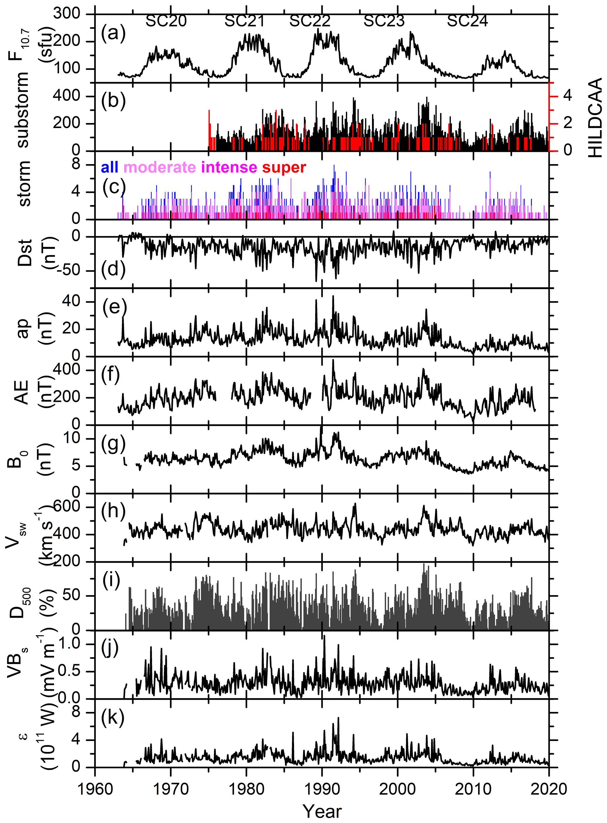
Figure 1 From top to bottom, the panels show (a) the monthly mean solar F_10.7 flux; (b) monthly numbers of substorms (black, legend on the left) and HILDCAAs (red, legend on the right); (c) geomagnetic storms of varying intensity; monthly mean (d) Dst, (e) ap, (f) AE, (g) IMF B₀, and (h) V_sw; (i) percentage of days with daily peak V_sw ≥ 500 km s⁻¹ (D₅₀₀); and monthly mean (j) VB_s and (k) Akasofu ϵ parameter, during 1963 to 2020. Solar cycles from SC20 to SC24 are marked on the top panel.

Monthly superposed variations

Figure 2 shows the monthly superposed values of all the parameters shown in Fig. 1. Figure 2a–f shows the numbers of geomagnetic events in each month divided by the number of years of observations (in the unit of number per year). Figure 2g–l shows the monthly means of the geomagnetic and solar wind/interplanetary parameters for the entire interval of study.

Figure 2 Monthly superposed variations. Left panels, from top to bottom, show the total numbers divided by years of observation of (a) substorms, (b) HILDCAAs, (c) all storms (AS), (d) moderate storms (MS), (e) intense storms (IS) and (f) super storms (SS), respectively. Right panels, from top to bottom, show the monthly mean values of the (g) geomagnetic Dst, (h) ap, and (i) AE indices; (j) IMF B₀; (k) V_sw (black, legend on the left) and D₅₀₀ (red, legend on the right); and (l) VB_s (black, legend on the left) and ϵ parameter (red, legend on the right), respectively.

The substorm occurrence rate (Fig. 2a) clearly exhibits two peaks during the months of March and October and a summer solstice minimum (during the month of June). HILDCAAs (Fig. 2b) do not exhibit any clear seasonal feature, except a significant minimum in November. Geomagnetic storms, from moderate to intense (Fig. 2d–e), exhibit a clear semi-annual variation. The spring equinoctial peak is recorded during March for the moderate storms and during April for the intense storms, while the fall peak is recorded during October for both of them. The super storms (Fig. 2f), with a very low occurrence rate, do not have any clear seasonal feature. As majority of the storms are of moderate intensity; storms of all intensity together (Fig. 2c) exhibit a prominent semi-annual variation with two peaks during March and October.

The monthly mean intensities of the Dst (Fig. 2g) and ap (Fig. 2h) indices show a semi-annual variation. Both of them exhibit the spring peaks during March. While Dst has a fall minimum during October, ap exhibits a peak during September. On the other hand, the monthly mean AE index (Fig. 2i) increases gradually from January; attains a peak around April; decreases with a much slower rate till September, after which the decrease rate is faster, and finally attains a minimum during December. Thus, the AE index shows an annual variation, different from the Dst and ap indices. This result is consistent with Katsavrias et al. (2016) who also reported an annual component in AE, and lack of any semi-annual component. As the AE index is based on geomagnetic observations made in the northern hemisphere, the asymmetric pole exposition to the solar radiation during the Earth's translational motion could contribute to this annual variation. The latter may modulate the AE current through the modulation of the ionospheric conductivity, owing to the solar extreme ultraviolet (EUV) ionization.

It is worth mentioning that the AE index (Davis and Sugiura, 1966) includes an upper envelope (AU) and a lower envelope (AL) related to the largest (positive) and smallest (negative) magnetic deflections, respectively, among the magnetometer stations used. The AU and AL components represent the strengths of the eastward and westward AE, respectively. Lockwood et al. (2020) showed that the semi-annual variation is indeed present in the AL index. As the auroral westward current represented by AL is associated with the substorm-related energetic particle precipitation in the auroral ionosphere, the semi-annual variation in AL is consistent with the semi-annual variation exhibited by the substorms (present work). On the other hand, the eastward auroral current/AU is mainly contributed by the dayside ionospheric conductivity that exhibits a summer solstice maximum as suggested by Wang and Lühr (2007) and Tanskanen et al. (2011).

Among the solar-wind–magnetosphere coupling parameters, VB_s (Fig. 2l, legend on the left) exhibits a semi-annual variation, with larger average values during February–April months, another sharp peak during October and with a solstice minimum. For the monthly mean IMF B₀ (Fig. 2j), a clear minimum can be noted during July, and B₀ increases gradually on both sides of July. No clear seasonal features can be inferred from the variations of the monthly mean V_sw (Fig. 2k, legend on the left) or Akasofu ϵ parameter (Fig. 2l, legend on the right). However, D₅₀₀ (Fig. 2k, legend on the right) exhibits two clear peaks around March and September, with prominently lower values during solstices.

Periodogram analysis

It should be noted that the seasonal features as described above (Fig. 2) present an average scenario composed by superposition of several solar cycles. The seasonal features may vary from one solar cycle to the other. In Fig. 3 we have performed the Lomb–Scargle periodogram analysis of the above events and parameters. For this purpose, we use the monthly means of F_10.7, Dst, ap, AE, B₀, V_sw, D₅₀₀, VB_s and ϵ, as well as the monthly numbers of substorms, HILDCAAs and magnetic storms of varying intensity. In the left panel of Fig. 3, the periodograms are based on the original data of 1-month resolution, while the right panel shows the periodograms after filtering out the dominating ∼11-year periodicity from the data. It can be noted that the filtering helps to better identify the shorter-scale periodicities in the time series.

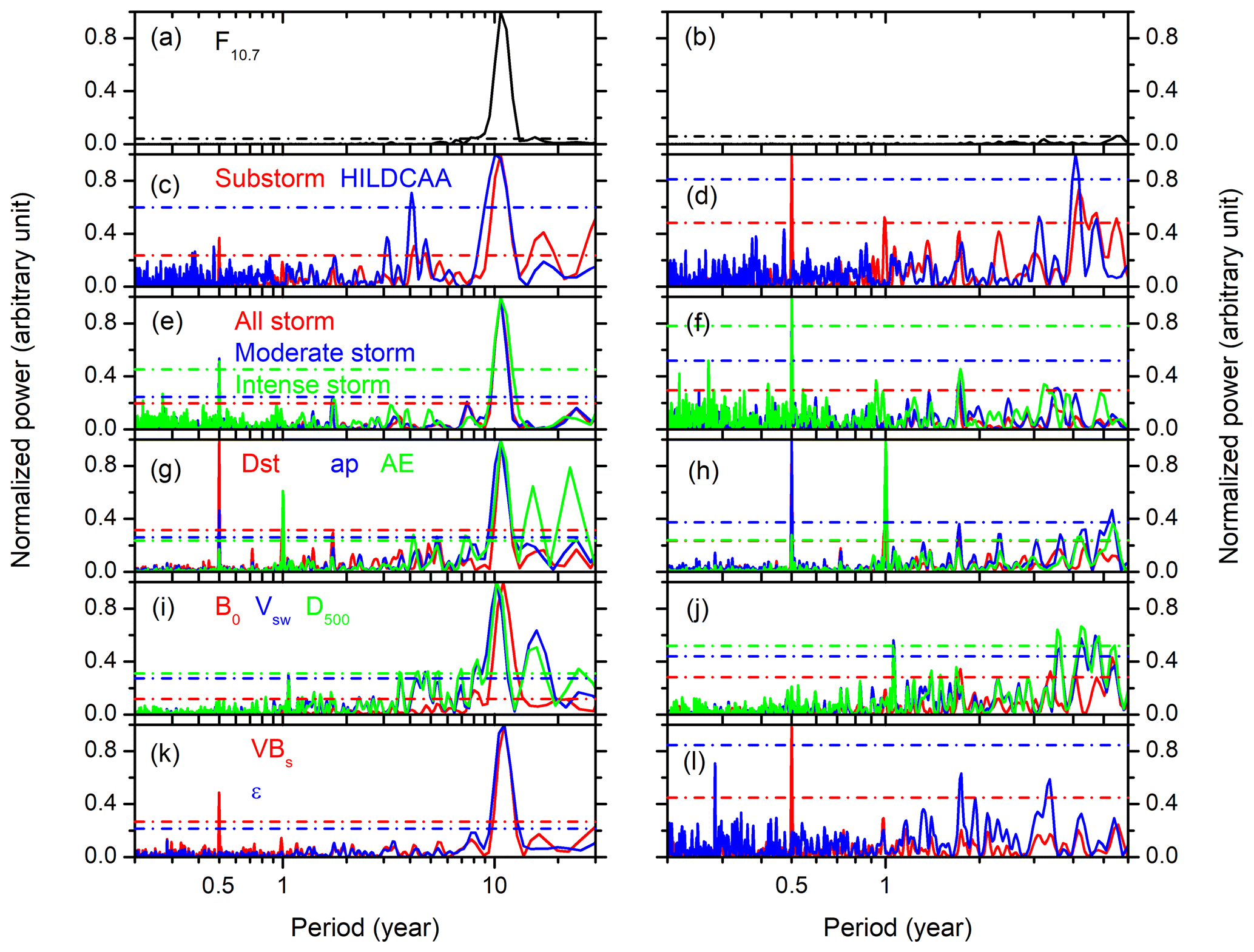
Figure 3 Lomb–Scargle periodograms. From top to bottom, the panels show the normalized power of periods for the monthly mean (a, b) solar F_10.7 flux; monthly numbers of (c, d) substorms and HILDCAAs; (e, f) all magnetic storms, moderate storms, and intense storms; monthly mean (g–h) geomagnetic indices Dst, ap, and AE; (i–j) solar wind parameters IMF B₀, V_sw, and D₅₀₀; and (k–l) VB_s and ϵ parameter, respectively. The left panels correspond to periodograms of the original database without any filtering, while the right panels correspond to periodograms after filtering out the 11-year periodicity from the database. Horizontal dot-dashed lines in each panel indicate >95% significance levels of the corresponding parameters shown by different colors. Note that the x axes have different scaling for the left and right panels.

As expected, the F_10.7 solar flux shows a prominent (at >95% significance level) ∼11-year periodicity (Fig. 3a) and no shorter-scale variation (Fig. 3b). A dominating ∼11-year periodicity can also be observed in substorms; HILDCAAs (Fig. 3c); magnetic storms of varying intensity (Fig. 3e); the geomagnetic indices Dst, ap, and AE (Fig. 3g); in the solar wind/interplanetary parameters IMF B₀, V_sw, and D₅₀₀ (Fig. 3i); and the solar-wind–magnetosphere coupling functions VB_s and ϵ (Fig. 3k). However, we are interested in the annual or shorter-scale periodicities in the events and parameters. Thus, the Lomb–Scargle periodograms are also performed after filtering out this dominating ∼11-year periodicity from the data. The same is shown in the right panel of Fig. 3.

Table 3 Significant (at the >95% level) periods less than ∼11 years obtained from the Lomb–Scargle periodogram analysis. Periods are ordered from higher power to lower.

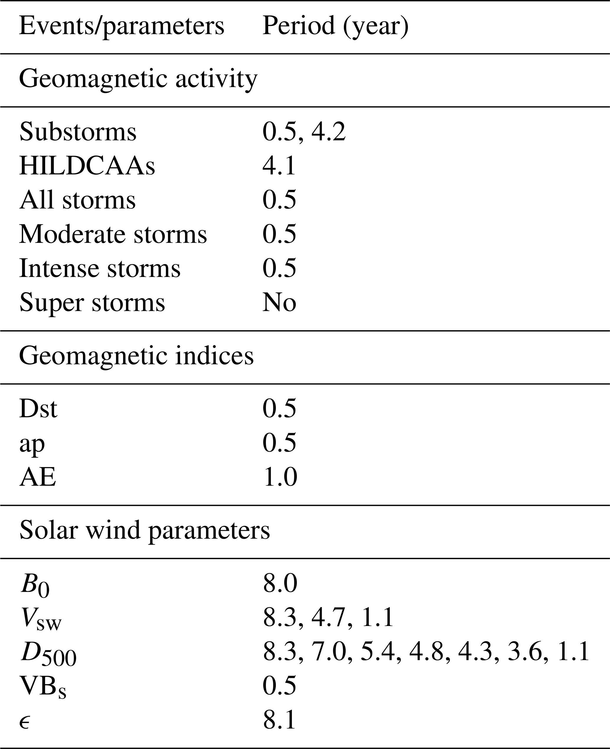
Table 3 lists the significant periodicities which are less than the ∼11-year solar cycle period. As clear from Fig. 3 and Table 3, substorms (Fig. 3d) and moderate and intense geomagnetic storms (Fig. 3f) exhibit prominent semi-annual (∼6-month period) variation. However, the super storms do not exhibit any clear variation pattern (not shown). HILDCAAs (Fig. 3d), on the other hand, exhibit a ∼4.1-year periodicity, while no annual or lower-scale variation was recorded. However, it should be noted that very low monthly numbers of HILDCAAs and super storms during different years may introduce significant artifacts to the corresponding spectral/periodogram analysis. Thus, the results of the periodogram analysis for HILDCAAs and super storms cannot be fully trusted.

Both the ap and Dst indices exhibit a clear ∼6-month periodicity (Fig. 3h). However, the AE index exhibits an annual variation but no semi-annual variation.

The solar wind/interplanetary and coupling functions exhibit more complex periodicity (lower than ∼11 years). The IMF B₀ (Fig. 3i) and ϵ parameter (Fig. 3k) exhibit ∼8-year periodicity but no annual or lower-scale periodicity (Fig. 3j and l). The solar wind V_sw and D₅₀₀ (Fig. 3j) exhibit several periodicities in the range of ∼4–8 years and a significant annual variation (periodicity ∼1 year). The coupling function VB_s exhibits a prominent semi-annual variation (Fig. 3l). The V_sw periodicities detected in the present work are consistent with results reported previously (e.g., Valdés-Galicia et al., 1996; El-Borie, 2002; El-Borie et al., 2020; Hajra, 2021a; Hajra et al., 2021, and references therein). For example, El-Borie (2002) reported ∼9.6-year periodicity in V_sw arising from the coronal hole variations in the southern hemisphere of the Sun. El-Borie et al. (2020) discussed multiple V_sw periodicities in the 1–2-, 2–4-, 4–8- and 8–16-year bands. Recently, Hajra et al. (2021) reported significant V_sw periodicities of ∼3, ∼4, ∼10 and ∼16 years and discussed their important role in space climatology.

The results shown in Fig. 3 and Table 3 are consistent with those in Fig. 2. From the above analyses, the coupling function VB_s which exhibits a ∼6-month periodicity can be inferred as the driver of the semi-annual variations in substorms, moderate and intense storms, and in the geomagnetic indices Dst and ap. On the other hand, the ∼1-year periodicity in V_sw/D₅₀₀ can be a source of the annual variation in the AE index. In addition, the ∼4.1-year periodicity in HILDCAAs seems to be associated with the solar wind V_sw variation in the same range. Detailed analyses of the events and/or parameters which exhibit the annual and/or semi-annual variations are shown in Sect. 3.2. For a detailed analysis of the longer-scale variations of the geomagnetic activity, the geomagnetic indices, and the solar-wind–magnetosphere coupling, which is beyond the scope of this present work, we refer the reader to Hajra et al. (2021).

3.2 Solar activity dependence

The solar cycle variations of the seasonal features described in Sect. 3.1 are explored in Figs. 4 to 11. They show the variations of the substorms (Fig. 4); the moderate (Fig. 5) and intense (Fig. 6) magnetic storms; the geomagnetic Dst (Fig. 7), ap (Fig. 8), and AE (Fig. 9) indices; the solar wind plasma speed V_sw (Fig. 10); and the coupling function VB_s (Fig. 11). The format is identical for all these figures: for the geomagnetic events (the solar wind/interplanetary parameters), panel c shows the year–month contour plot of the number of the events (the mean values of the parameters) in each month of the observing years. The values of different colors are given in the legend at the bottom. Panel d shows the yearly mean F_10.7 solar flux. The solar minima are marked by the horizontal dot-dashed lines in the bottom panels c–d. Panel b shows the monthly numbers of the events per a year of observation (the monthly mean values of the parameters) during each solar cycle, while panel a shows the same during groups of the even, odd, strong, weak and all solar cycles.

Table 4 Seasonal modulation (%) between the equinoctial maximum and the solstice minimum for the events and the parameters with the semi-annual variation during the weak and strong solar cycles, as well as the odd and even solar cycles (defined in Sect. 2).

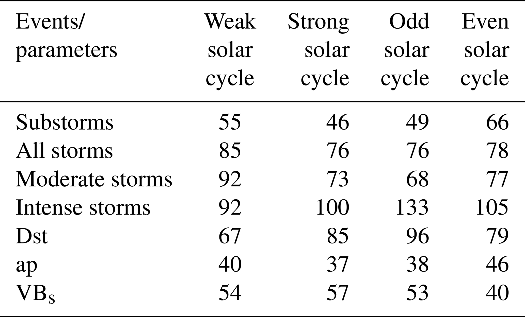
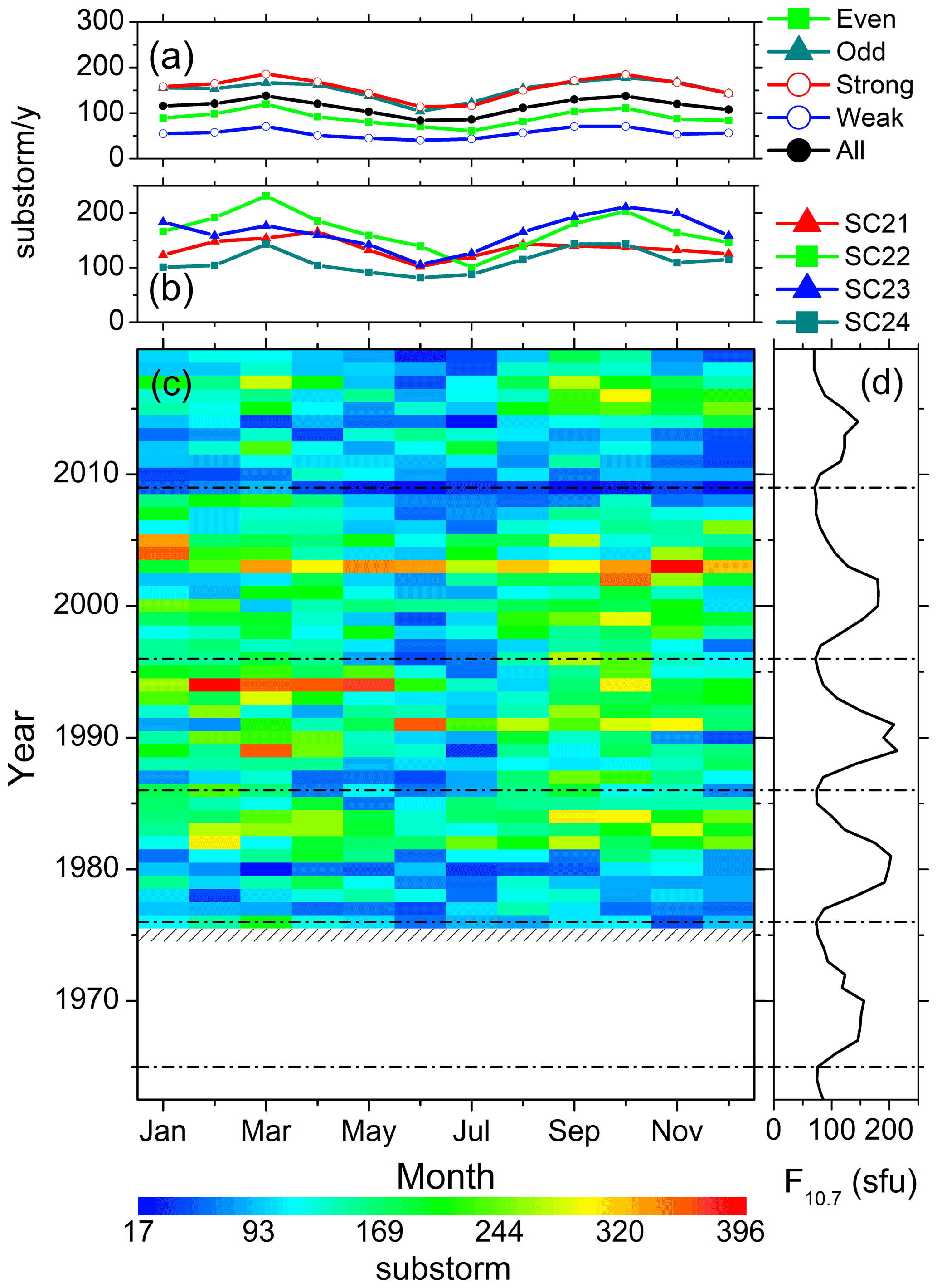
Figure 4 Substorms from 1976 to 2019. Panel (c) shows the year–month contour plot of the number of substorms in each month of the years 1976–2019. The values of different colors are given in the legend at the bottom. Data gaps are shown by crosses. Panel (d) shows the yearly mean F_10.7 solar flux. Panel (b) shows the monthly numbers of substorms per a year of observation during each solar cycles, and panel (a) shows the same during groups of the even, odd, strong, weak and all solar cycles. For details on the grouping of the solar cycles, see the text. The solar minima are marked by horizontal dot-dashed lines.

Table 4 lists a “seasonal modulation” parameter defined as the difference between the equinoctial maximum and the solstice minimum expressed as the percentage of the yearly mean value for the events and parameters exhibiting the semi-annual variation. The modulation parameter can be taken as a measure of the seasonal/semi-annual variability. The larger the value of the parameter, the stronger the semi-annual variability. Large variation in the seasonal modulation can be noted from the table. For substorms, all storms, moderate storms and the ap index, seasonal modulations are larger during the weak cycles (even cycles) than the strong cycles (odd cycles). However, the modulations are larger during the strong cycles (odd cycles) than the weak cycles (even cycles) for the intense storms, the Dst index and the coupling function VB_s. The explanation is not known at present. However, it is interesting to note that the intense storms (and thus the strong Dst associated with intense VB_s) are mainly driven by the interplanetary coronal mass ejections (ICMEs). On the other hand, the moderate storms, substorms, and the ap index variations are associated with both ICMEs, and the corotating interaction regions (CIRs) between the slow streams and HSSs (e.g., Tsurutani and Gonzalez, 1987; Tsurutani et al., 1988; Gosling et al., 1990; Richardson et al., 2002; Echer et al., 2008; Hajra et al., 2013; Souza et al., 2016; Mendes et al., 2017; Marques de Souza et al., 2018; Tsurutani et al., 2019, and references therein). The strong cycles are expected to be characterized by more solar transient events like ICMEs than during the weak cycles. However, recent studies show lower numbers and reduced geoeffectiveness of both CIRs and ICMEs during the weak cycles than during the strong cycles (e.g., Scolini et al., 2018; Grandin et al., 2019; Lamy et al., 2019; Nakagawa et al., 2019; Syed Ibrahim et al., 2019; Hajra, 2021c, and references therein). This calls for a further study to explain the above results.

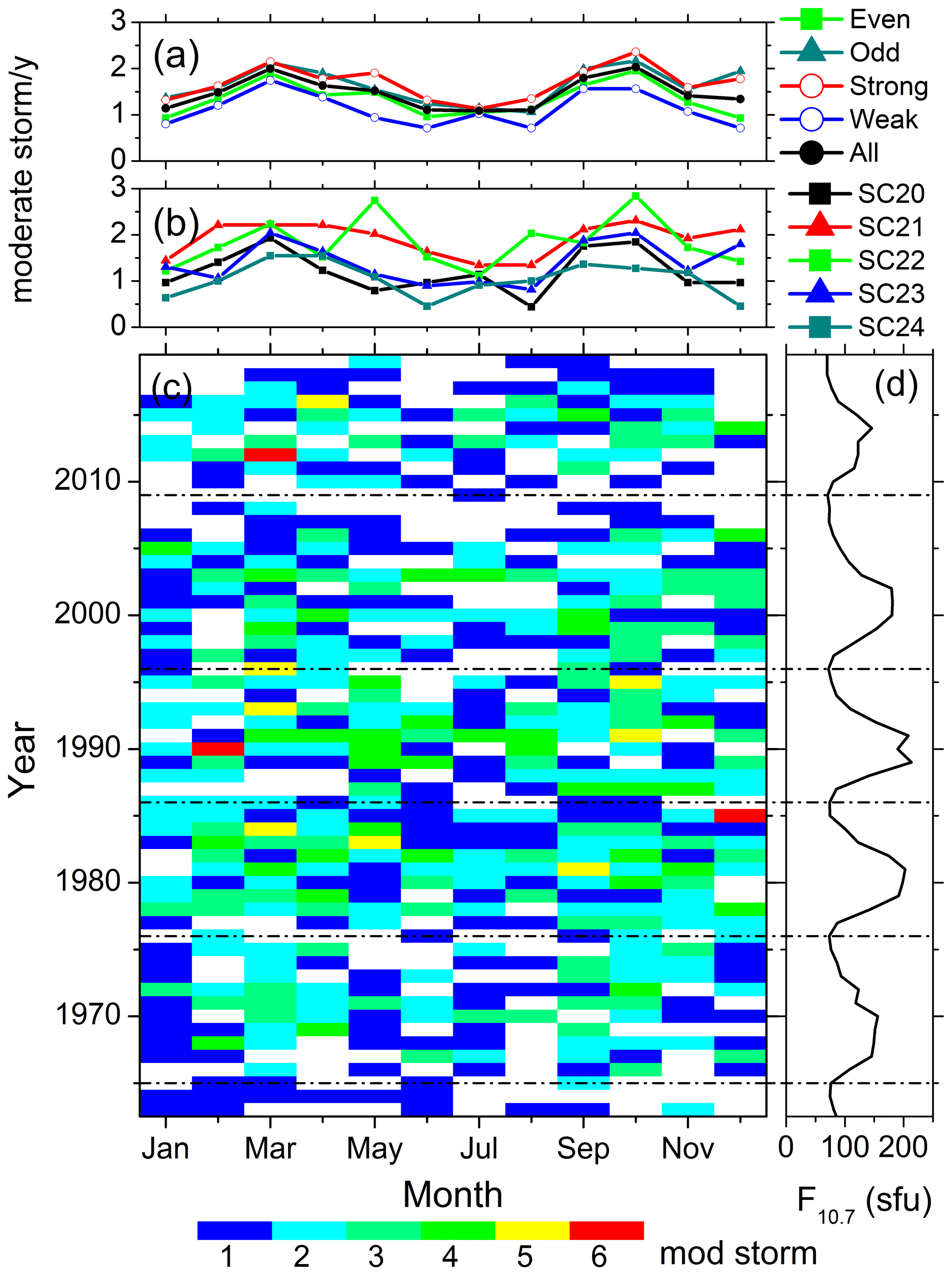
Figure 5 Moderate geomagnetic storms from 1963 to 2019. The panels are in the same format as in Fig. 4.

3.2.1 Substorms

From Fig. 4c it can be seen that in any solar cycle, the peak substorm occurrence rates are noted during the descending phase, followed by the occurrence minimum during the solar minimum to early ascending phase. From the four complete solar cycles (SC21–SC24) of the substorm observations, two prominent peaks can be noted in the years of 1994 and 2003, which are in the descending phases of SC22 and SC23, respectively.

On the seasonal basis, two peaks around the months of March and October can be observed from the year–month contour plot (Fig. 4c), which is also reflected in the monthly superposed plots (Fig. 4a–b). However, this “semi-annual” variation exhibits a large asymmetry in amplitude and duration between the spring and fall equinoxes. For example, in the year 1994, the substorm occurrence peak during February–May is significantly larger than the occurrences during October. On the other hand, during 2003, while the occurrence peak is noted in November, comparable occurrences are clear almost during the entire year.

When separated on the basis of the solar cycles (Fig. 4a–b), the smallest numbers of events are observed during SC24. Interestingly, the spring occurrences are the strongest in SC22 and the fall occurrences are the strongest in SC23. Another noteworthy feature is that the occurrence rates during the even and weak solar cycles are lower than during the odd and strong cycles, respectively. However, the seasonal modulation between the equinoctial maximum and the solstice minimum is comparable between the weak (∼55 %) and strong (∼46 %) cycles (Table 4).

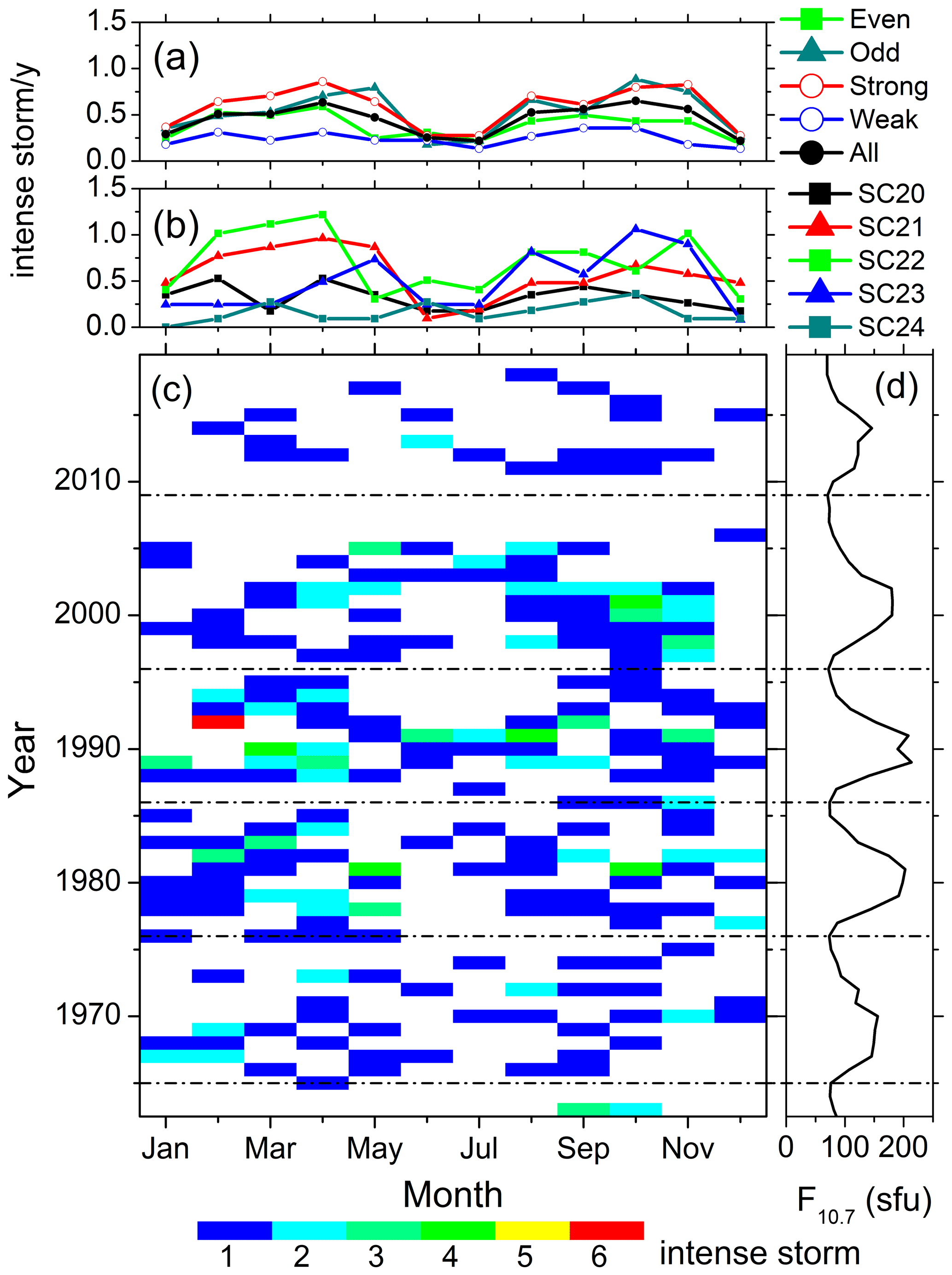
3.2.2 Geomagnetic storms

Variations of the moderate and intense geomagnetic storms are shown in Figs. 5 and 6, respectively. From the year–month contour plots (Figs. 5c and 6c), the moderate storms are found to peak around the descending phases, while the intense storms peak around the solar maximum. When the monthly variations of the storms are considered in each year, there is hardly any seasonal variation. However, when observations during several solar cycles are grouped together (Figs. 5a and 6a), the semi-annual variation can be noted in the moderate storms. There is not much difference in moderate and intense storm occurrence rates between the odd and even cycles. However, the occurrence rates of the storms are slightly larger in the strong cycles compared to the weak ones, while the seasonal modulation between the equinoctial maximum and the solstice minimum during the strong and weak cycles is comparable (Table 4). Another noteworthy feature is the lowest occurrence of intense storms during SC24.

Figure 6 Intense geomagnetic storms from 1963 to 2019. The panels are in the same format as in Fig. 4.

3.2.3 Geomagnetic indices

Variations of the monthly mean geomagnetic indices are shown in Figs. 7 (Dst), 8 (ap) and 9 (AE). In each solar cycle, the average Dst index exhibits the strongest negative excursions at and immediately after the solar maximum (Fig. 7c–d). A clear correlation can be observed between the F_10.7 solar flux and the average Dst strength. The Dst negative excursions are stronger during the strong and odd cycles compared to the weak and even cycles, respectively (Fig. 7a). In addition, the seasonal modulation between the equinox minimum to the solstice maximum is significantly higher in the strong cycles (∼85 %) compared to the weak cycles (∼67 %) (Table 4). During SC24, the overall Dst strength is the weakest and there is no prominent seasonal modulation.

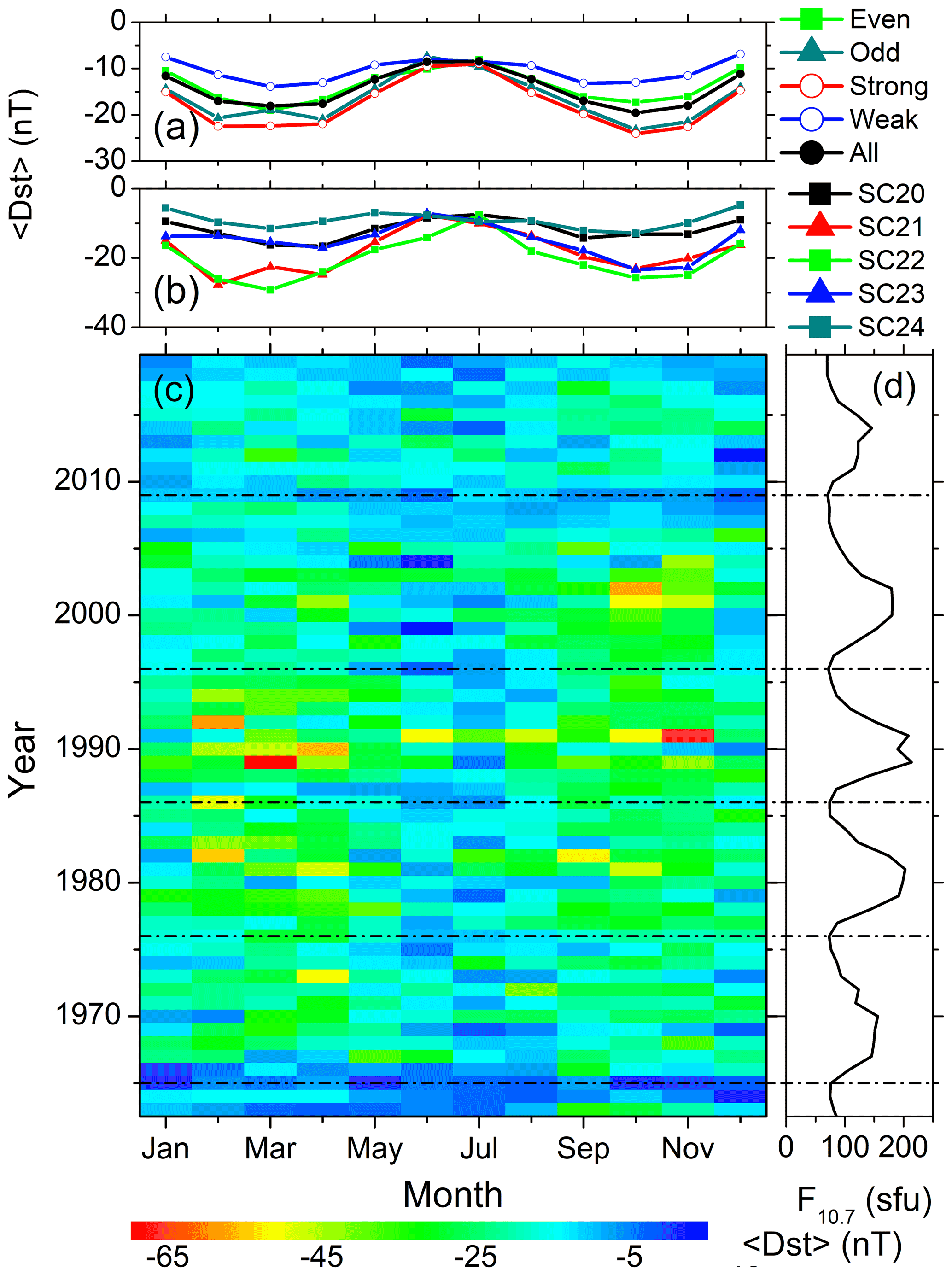
Figure 7 Geomagnetic Dst index variation from 1963 to 2019. Panel (c) shows the year–month contour plot of the mean Dst value in each month of the years 1963–2019. The values of different colors are given in the legend at the bottom. Data gaps are shown by crosses. Panel (d) shows the yearly mean F_10.7 solar flux. Panel (b) shows the monthly means of Dst during each solar cycles, and panel (a) shows the same during groups of the even, odd, strong, weak and all solar cycles.

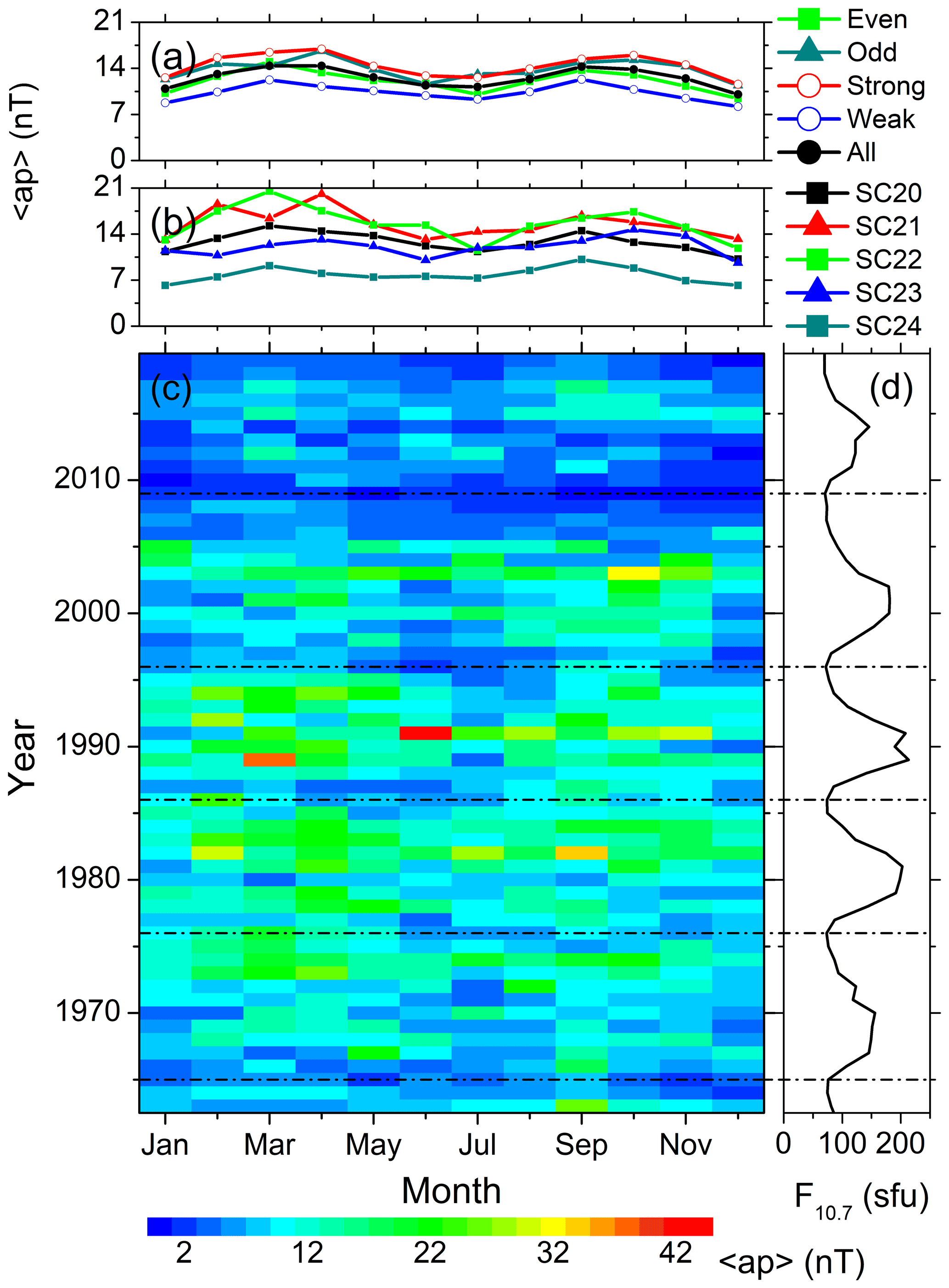
Figure 8 Geomagnetic ap index variation from 1963 to 2019. The panels are in the same format as in Fig. 7.

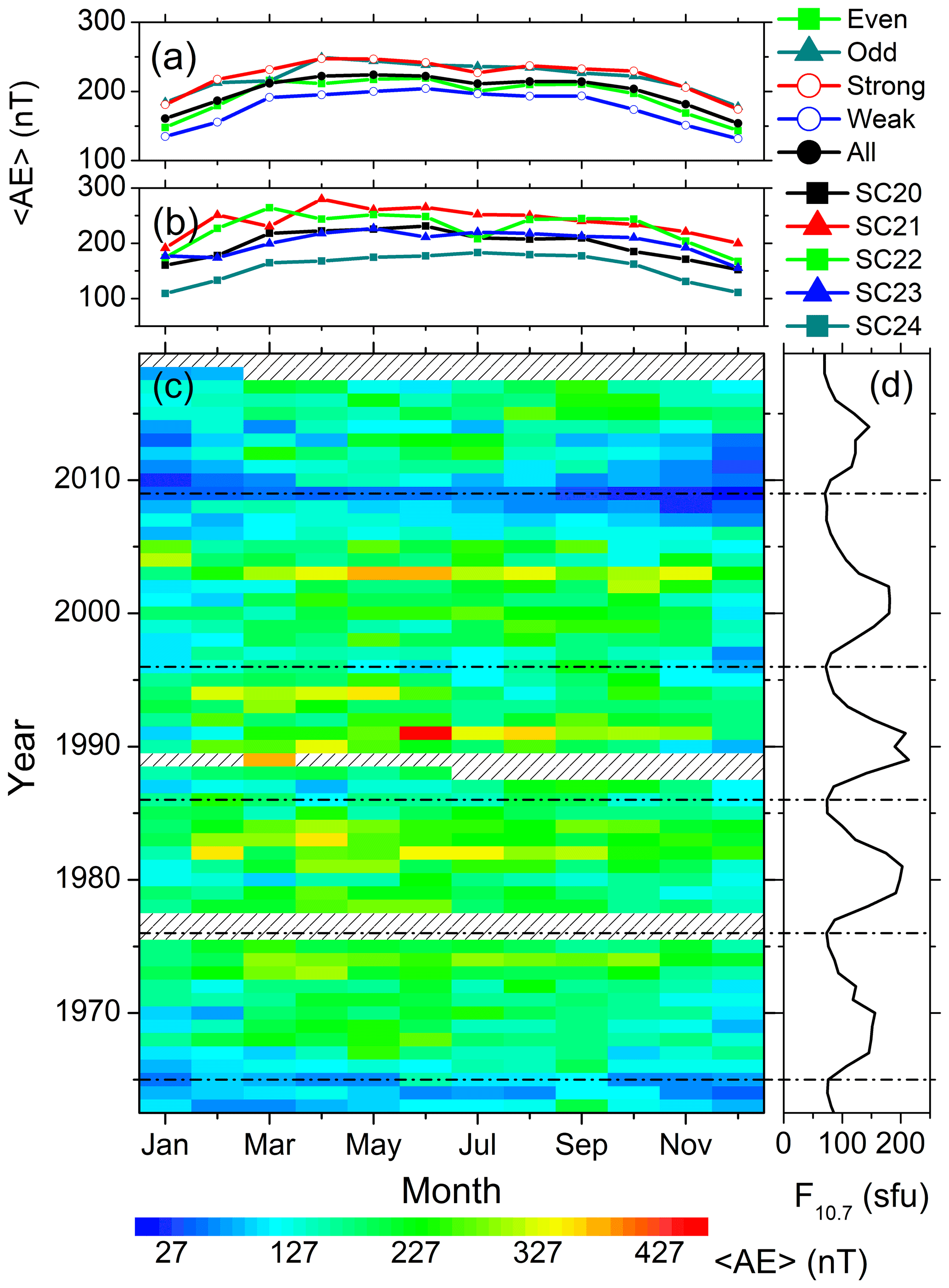
Figure 9 Geomagnetic AE index variation from 1963 to 2019. The panels are in the same format as in Fig. 7.

Variation of the monthly mean ap index (Fig. 8) is identical to the Dst index variation. However, the seasonal modulation is comparable between the strong (∼37 %) and weak (∼40 %) cycles for the ap index (Table 4).

Variation of the AE index (Fig. 9) is significantly different than the variations of the Dst and ap indices. In a solar cycle, AE peaks around the descending phase (Fig. 9c). On the yearly basis, the average AE values are enhanced from March/April to September/October. The summer solstice values are significantly higher compared to the winter solstice values. This indicates an annual variation, in agreement with the Lomb–Scargle periodogram analysis result (Fig. 3h). There is no semi-annual variation. The average values during the strong and odd solar cycles are higher compared to the weak and even solar cycles, respectively (Fig. 9a). SC24 exhibited the lowest values of AE compared to other solar cycles (Fig. 9b).

3.2.4 Solar-wind–magnetosphere coupling

The periodogram analysis (Fig. 3j and Table 3) identified a weak annual component in the variations of the solar wind speed V_sw (compared with its stronger amplitude longer-scale variations). The monthly mean values of V_sw during each year of observation are shown in Fig. 10c. In a solar cycle, V_sw peaks around the descending phase, indicating a higher occurrence rate of HSSs during this phase. This is also confirmed by the variations of D₅₀₀ (not shown). Interestingly, during the descending phase of SC20, the V_sw peak can be noted around March–April; during the SC21 descending phase, two equinoctial peaks are almost symmetric; during the SC22 descending phase, peaks are recorded during the first half of the year; the peaks shift to the second half of the year during the SC23 descending phase; and during the SC24 descending phase, no prominent feature can be inferred. Thus, overall, a shift of the seasonal peak of V_sw from the first half to the second half of the year can be observed between the even and the odd cycles. In addition, during the first half of the year, the average values are significantly high during the odd and strong cycles than during the even and weak cycles, respectively (Fig. 10a).

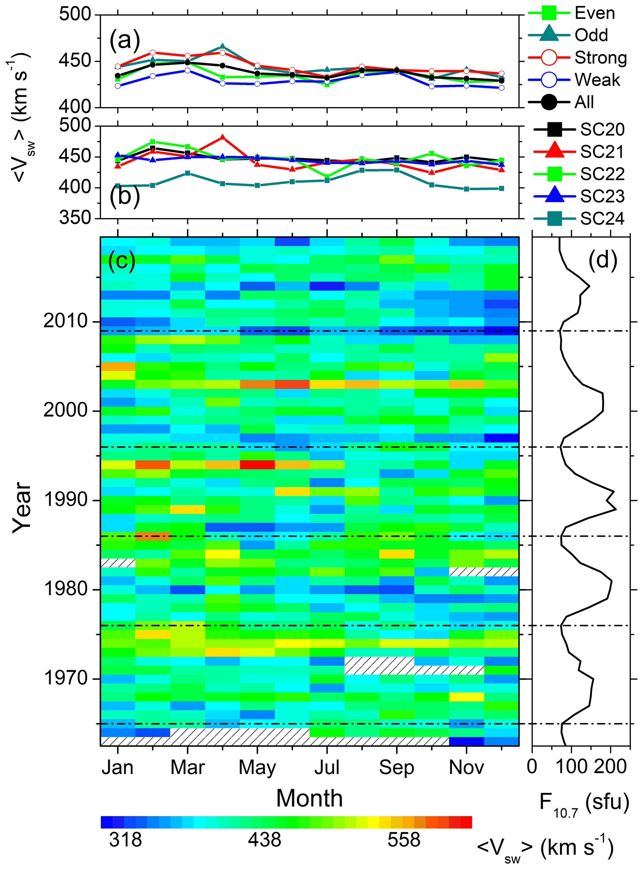
Figure 10 Solar wind speed V_sw variation from 1963 to 2019. The panels are in the same format as in Fig. 7.

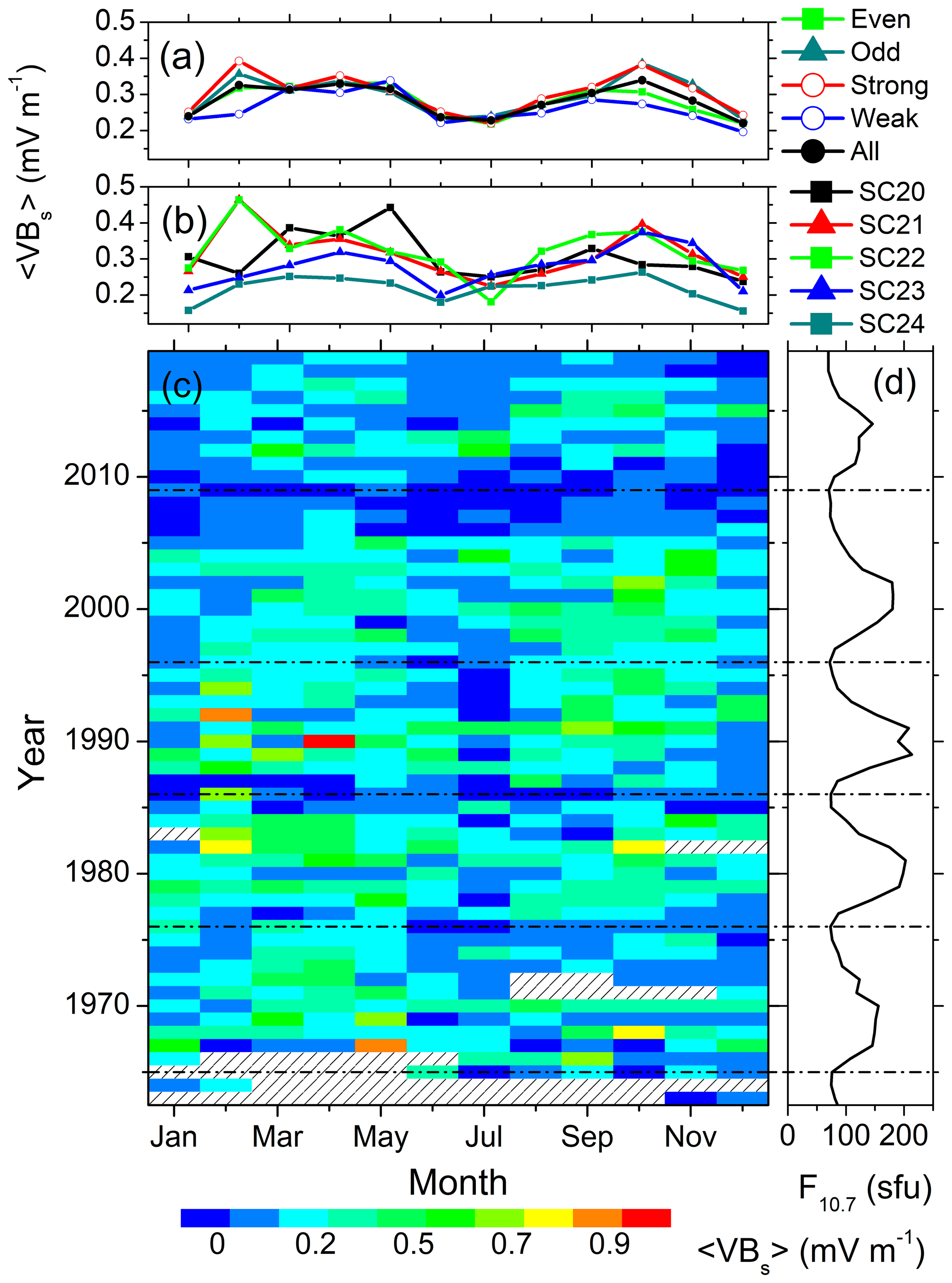
Figure 11 Solar wind coupling function VB_s variation from 1963 to 2019. The panels are in the same format as in Fig. 7.

Figure 11 shows the monthly mean values of the coupling function VB_s during all years of observation. In a solar cycle, VB_s peaks around the solar maximum, when almost symmetrical peaks can be observed during the equinoxes and minima during the solstices (Fig. 11c). The lowest values of VB_s are recorded during SC24 (Fig. 11b). There is no prominent difference between the weak and strong cycles, or between the even and odd cycles, except that the February and October values are higher during the odd and strong cycles compared to those during the even and weak cycles, respectively (Fig. 11a).

4 Conclusions

We used an up-to-date database of substorms, HILDCAAs and geomagnetic storms of varying intensity along with all available geomagnetic indices during the space exploration era (i.e., after 1957) to explore the seasonal features of the geomagnetic activity and their drivers. No such study involving such a long database and all types of geomagnetic activity has been reported before. As substorms, HILDCAAs and magnetic storms of varying intensity have varying solar/interplanetary drivers; such a study is important for a complete understanding of the seasonal features of the geomagnetic response to the solar/interplanetary events. The main findings of this work are discussed below.

First, the semi-annual variation is not a “universal” feature of the geomagnetic activity. While the monthly numbers of substorms and moderate and intense magnetic storms exhibit the semi-annual variation with two equinoctial maxima and a summer solstice minimum, super storms (with a very low occurrence rate) and HILDCAA events do not exhibit any clear seasonal dependence. For geomagnetic indices, the monthly mean ring current index Dst and the global geomagnetic activity index ap exhibit the semi-annual variation, while the auroral ionospheric electrojet current index AE exhibits an annual variation with a summer solstice maximum and a winter minimum. These results clearly demonstrate varying solar, interplanetary, magnetospheric and ionospheric processes behind different geomagnetic events and indices. While the magnetic reconnection (Dungey, 1961) between the southward IMF and the northward (dayside) geomagnetic field is the key for any geomagnetic effect, variations in the reconnection process and modulation by other processes may result in different geomagnetic effects (e.g., Gonzalez et al., 1994; Tsurutani et al., 2020; Hajra, 2021a; Hajra et al., 2021, and references therein). In general, major magnetic storms are associated with strong magnetic reconnection continuing for a few hours, while weaker reconnection for an hour or less can cause substorms. On the other hand, discrete and intermittent magnetic reconnection continuing for a long interval of time may lead to HILDCAAs (see Gonzalez et al., 1994, for a detailed comparison).

We observe a clear semi-annual component in the coupling function VB_s, which represents the reconnection electric field or the magnetic flux transfer rate into the magnetosphere. On the other hand, the solar wind speed V_sw does not have any semi-annual component, only annual and longer-scale components. As the main focus of the present work is the seasonal features, we refer the reader to previous works for a discussion on the longer-scale variations in V_sw (e.g., Valdés-Galicia et al., 1996; El-Borie, 2002; El-Borie et al., 2020; Hajra, 2021a, c; Hajra et al., 2021, and references therein). However, this result is very interesting. This clearly implies that the solar wind does not have any intrinsic semi-annual variation and that the semi-annual variation in VB_s is due to magnetic configuration (B_s) as suggested previously (e.g., Cortie, 1912; McIntosh, 1959; Boller and Stolov, 1970; Russell and McPherron, 1973). The VB_s semi-annual variation is suggested to cause the semi-annual variations of the substorms, the moderate and intense storms, and the geomagnetic Dst and ap indices. On the other hand, absence of any clear seasonal features in the super storms and HILDCAAs indicates more complex solar wind and magnetic coupling process during these events, which needs further study. As previously established, HILDCAAs are associated with HSSs emanated from the solar coronal holes (e.g., Tsurutani and Gonzalez, 1987; Hajra et al., 2013). Dominating longer-scale variations in V_sw (as revealed in the present work) may be a plausible reason for the ∼4.1-year variation and lack of any seasonal feature in HILDCAAs (Hajra et al., 2014a; Hajra, 2021c). Annual variation in the auroral ionospheric AE index, as mentioned before, may be attributed to a combined effect of the solar wind V_sw variation, the asymmetric pole exposition to the solar radiation, and the ionospheric conductivity variations (see, e.g., Wang and Lühr, 2007; Tanskanen et al., 2011).

In addition to the above, we found a complex solar activity dependence of the abovementioned seasonal features. The spring–fall asymmetry in substorms and the average V_sw variation between the odd and even solar cycles are consistent with results reported by Mursula et al. (2011). An interesting and puzzling result is observed in terms of variations in the semi-annual variability (seasonal modulation between the equinoctial maximum and the solstice minimum) between the strong (odd) and weak (even) solar cycles. While the seasonal modulation in substorms, all storms, moderate storms and the ap index is larger during the weak (and even) solar cycles compared to the strong (and odd) solar cycles, the reverse is true for the intense storms, the Dst index and the coupling function VB_s. At present we do not know the exact mechanism behind this result. In fact, further study is required for a better understanding of the solar cycle dependencies of the geomagnetic activity seasonal features. In conclusion, this study, along with several previous works (e.g., Mursula et al., 2011; Hajra et al., 2013, 2016; Hajra, 2021b), calls for a careful reanalysis of the solar, interplanetary, magnetospheric and ionospheric observations before applying the theoretical semi-annual models.