the Creative Commons Attribution 4.0 License.
the Creative Commons Attribution 4.0 License.
 | 14 Oct 2021
Validation of SSUSI-derived auroral electron densities: comparisons to EISCAT data
Patrick J. Espy
Larry J. Paxton
The coupling of the atmosphere to the space environment has become recognized as an important driver of atmospheric chemistry and dynamics. In order to quantify the effects of particle precipitation on the atmosphere, reliable global energy inputs on spatial scales commensurate with particle precipitation variations are required. To that end, we have validated auroral electron densities derived from the Special Sensor Ultraviolet Spectrographic Imager (SSUSI) data products for average electron energy and electron energy flux by comparing them to EISCAT (European Incoherent Scatter Scientific Association) electron density profiles. This comparison shows that SSUSI far-ultraviolet (FUV) observations can be used to provide ionization rate and electron density profiles throughout the auroral region. The SSUSI on board the Defense Meteorological Satellite Program (DMSP) Block 5D3 satellites provide nearly hourly, 3000 km wide high-resolution (10 km×10 km) UV snapshots of auroral emissions. These UV data have been converted to average energies and energy fluxes of precipitating electrons. Here we use those SSUSI-derived energies and fluxes as input to standard parametrizations in order to obtain ionization-rate and electron-density profiles in the E region (90–150 km). These profiles are then compared to EISCAT ground-based electron density measurements. We compare the data from two satellites, DMSP F17 and F18, to the Tromsø UHF radar profiles. We find that differentiating between the magnetic local time (MLT) “morning” (03:00–11:00 MLT) and “evening” (15:00–23:00 MLT) provides the best fit to the ground-based data. The data agree well in the MLT morning sector using a Maxwellian electron spectrum, while in the evening sector using a Gaussian spectrum and accounting for backscattered electrons achieved optimum agreement with EISCAT. Depending on the satellite and MLT period, the median of the differences varies between 0 % and 20 % above 105 km (F17) and ±15 % above 100 km (F18). Because of the large density gradient below those altitudes, the relative differences get larger, albeit without a substantially increasing absolute difference, with virtually no statistically significant differences at the 1σ level.
- Article
(2494 KB) - Full-text XML
- BibTeX
- EndNote


Particle precipitation and the processes initiated in the middle and upper atmosphere have been recognized as one ingredient to natural climate variability and are included in the most recent climate prediction simulations initiated by the Intergovernmental Panel on Climate Change (IPCC) (Matthes et al., 2017). So far, however, most of the studies are based on in situ particle observations at satellite orbital altitudes (≈800 km) (e.g. Wissing and Kallenrode, 2009; van de Kamp et al., 2016; Smith-Johnsen et al., 2018) or on trace-gas observations (Randall et al., 2009; Funke et al., 2017). In addition, most recent studies focus on the influence of “medium-energy” electrons (30–1000 keV) (Smith-Johnsen et al., 2018) that have their largest impact in the mesosphere (⪅90 km), but those occur more sporadically and have lower flux levels than typical lower energy auroral electrons.
Here we present a method to estimate the auroral particle input from 90–150 km, which is not only larger than the medium-energy input, but also occurs more regularly and persists throughout the night. Subsequent chemical reactions result in auroral particle precipitation being a major source of thermospheric NOx (Brasseur and Solomon, 2005), which can directly and indirectly influence the atmospheric ozone (Randall, 2005; Randall et al., 2009; Funke et al., 2005). To date, the impacts of this thermospheric source of aurorally produced reactive odd nitrogen (NOx) on the lower atmosphere are uncertain due to the insufficient altitude, spatial, and temporal sampling of currently used observations to characterize its source function and transport to the stratosphere (e.g. Randall et al., 2001, 2009). Using direct auroral observations will help to elucidate and quantify the production of auroral NOx with high spatio-temporal resolution, in particular as potential input for chemistry–climate models to trace the transport.
The Special Sensor Ultraviolet Spectrographic Imager (SSUSI) is one of the “Special Sensor” instruments on each of the Defense Meteorological Satellite Program (DMSP) Block-5D3 satellites F17 and F18 (Paxton et al., 1992, 2017, 2018). These satellites orbit at 850 km altitude in polar, sun-synchronous orbits with equator crossing times of the ascending nodes of 17:34 LT (F17) and 20:00 LT (F18). The orbital period is of the order of 100 min, such that an approximately 3000 km wide swath of the auroral zone is pictured multiple times by each satellite during a single night. The latest DMSP-5D3 satellites, F17–F19, were launched in 2006 (F17), 2009 (F18), and 2014 (F19). Here we compare the data from F17 and F18 to the ground-based measurements because control over F19 was lost in February 2016, and the observation time of F19 was apparently too short to facilitate a meaningful comparison.
The EISCAT (European Incoherent Scatter Scientific Association) incoherent scatter radars (ISRs) are located in northern Europe. They are located in Kiruna in Sweden, Sodankylä in Finland, Tromsø in Norway, and Longyearbyen on Svalbard. Thus they are positioned approximately in the auroral zone at low and moderate geomagnetic activity, providing measurements of the ionospheric composition such as electron and ion densities and temperatures.
In a previous study, Aksnes et al. (2006) compared EISCAT radar data and UV-derived satellite data during a single day. The satellite data were derived from the SSUSI predecessor sensors called UVI (Ultraviolet Imager; Torr et al., 1995), and the study validated the optical approach, at least for moderate geomagnetic activity. In their study, Aksnes et al. (2006) compared the far-ultraviolet (FUV)-derived electron density profiles from 105 to 155 km, with generally good agreement between UVI and EISCAT. They achieve that by individually choosing the precipitating electron spectrum for the UVI profiles that best reproduces the EISCAT profiles during that single substorm event.
A recent study by Knight et al. (2018) compared SSUSI-derived electron density parameters to ionosonde data. The altitude (hmE) and magnitude (NmE) of the ionospheric E layer derived directly from the SSUSI UV observations were compared with the same parameters derived from the ionosondes. Their extensive analysis also found a good agreement between these parameters above four ionosonde stations at auroral latitudes longitudinally distributed around the globe. That study also contains an extensive review about the conversion of the SSUSI FUV data to the precipitating electron characteristics. In a follow-up study, Knight (2021) also investigated the contribution of proton precipitation to the auroral emissions, finding a lower impact of protons than expected.
Here we use the SSUSI data for a full statistical investigation similar to the study presented by Knight et al. (2018), extending the earlier study by Aksnes et al. (2006) to multiple local times and auroral conditions. We also base our calculation on the approach presented in Aksnes et al. (2006), using the more recent ionization rate parametrizations introduced by Fang et al. (2010).
The paper is organized as follows: Sect. 2 introduces the SSUSI satellite data and the EISCAT radar data. In Sect. 3 we present the details of the comparison method, in Sect. 4 we present our results, and we discuss them in Sect. 5. Our conclusions are then presented in Sect. 6.
2.1 SSUSI UV and electron data
The SSUSI instruments remotely image the FUV auroral emissions (Paxton et al., 1992, 1993, 2002; Paxton and Zhang, 2016; Paxton et al., 2017). By scanning approximately ±60∘ across track (Paxton et al., 1993), the SSUSI instruments observe the auroral zone on an approximately 3000 km wide swath. The single pixel resolution is 10×10 km2 at the nadir point, and the scans extend from about 50∘ polewards in both hemispheres. The instantaneous field of view of the imaging spectrograph is 11.8∘, with 16 pixels along track, and overlapping across-track scans comprise the auroral swath as described in Paxton et al. (1992, 1993). The procedure also accounts for off-nadir effects in the FUV emissions (Paxton et al., 2017), and the processing steps are outlined in Paxton et al. (1993).
The SSUSI sensors record the FUV spectrum from 115 to 180 nm (Paxton et al., 1992), and they use in-flight calibration using a FUV star spectrum with well-understood brightness and spectral shape (Paxton et al., 2017). The downlink is limited to five channels with spectral centres at 121.6 nm (atomic hydrogen H Lyman-α), 130.4, and 135.6 nm (both atomic oxygen OI) and two channels for the N2 Lyman–Birge–Hopfield system (LBH), centred at 145 nm (140–150 nm, LBH-S) and 172.5 nm (165–180 nm, LBH-L). These channels capture the main auroral UV emissions and are used to calculate the average electron energy, (in keV), and total electron energy flux, Q0 (in (mW m−2)), at each pixel (Strickland et al., 1983, 1999; Knight et al., 2018).
Here we use the data from the SSUSI sensors on board the DMSP F17 and F18 satellites over their respective operating periods from 2008–2019 and from 2011–2019. In particular, we use the SSUSI Level-2 “Auroral-EDR” (Environmental Data Record) data product for auroral electron energy and energy flux, which are derived from the N2 LBH bands (Strickland et al., 1983). These quantities are provided in the environmental data records on a geomagnetic grid with a spacing of approximately 10 km×10 km. The general algorithm for the SSUSI data is based on Strickland et al. (1999) and is described in Knight et al. (2018) and in detail in the SSUSI data product algorithm descriptions (available at https://ssusi.jhuapl.edu/data_algorithms, last access: 17 June 2021). For comparison to EISCAT data, only data points within (latitude×longitude) of the radar's geomagnetic location were used. In addition, we require the average energy to be within the valid regime ( keV) and the derived energy flux Q0 to be non-zero.
This corresponds to the range over which one can determine the characteristic energy of the precipitating electrons just based on the ratio of LBH long, assumed to have little or no O2 absorption, to the LBH short, which is assumed to be attenuated by O2. “Soft” electrons, meaning low energy, dissipate their energy high in the atmosphere, and there is no O2 absorption in the LBH short or long. This means the ratio is almost constant, and determining the characteristic energy below about 2 keV becomes ambiguous. As the characteristic energy increases, the electrons are deposited deeper in the atmosphere. Eventually the N2 LBH long emissions start to get attenuated, and deducing the flux from LBH long becomes ambiguous. This attenuation starts to become important at and below the deposition altitudes for 20 keV electrons, approximately 90 km (Germany et al., 1990).
In addition, quenching losses of the N2 LBH emissions constitute about 20 % of the total deactivations at 90 km, and cascade and collisional energy transfer begin to occur, which can also distort the spectral distribution of the LBH. While the modelling based on Strickland et al. (1999) includes both quenching and O2 absorption, the complexity of the energy transfer in the singlet systems of the N2 molecule (Ajello et al., 2020) made it prudent to limit the energy range retrieved from SSUSI to 20 keV to avoid large corrections. For 20 keV electrons, the LBH emission falls extremely rapidly below 90 km (Germany et al., 1990).
2.2 EISCAT electron densities
We use data from the Tromsø UHF radar, which is located at N and E, in the auroral zone. The Tromsø radars include both transmitter and receiver, enabling them to provide altitude-resolved profiles of several ionospheric parameters, such as electron density, electron temperature, ion temperature, and many others, above the location using the incoherent scatter radar technique (Robinson and Vondrak, 1994; Lehtinen and Huuskonen, 1996). Depending on the so-called “pulse code” used for the “experiment”, the altitude resolution can be less than 200 m, but more typical in our comparison is ≈5 km. In addition, the antennas of the Tromsø radars can be pointed in different directions and different altitudes.
We use the publicly available EISCAT E-region electron density data from the Tromsø UHF radar. The data are available via the “Madrigal” database at http://cedar.openmadrigal.org (last access: 21 September 2020). The data are averaged ±5 min around the SSUSI scan time, and only high elevation angles ≥75∘ were considered. This time window was chosen so that several EISCAT profiles could be averaged to characterize the mean level of auroral ionization in the larger comparison region. No distinction between the different experiments (including scanning experiments) was made as long as there were electron densities available from at least 80 km and above, and all scans that provided those electron densities were interpolated onto a common 1 km altitude grid before averaging.
There are a number of methods for treating atmospheric ionization from particle precipitation. These include multi-stream calculations (Basu et al., 1993; Strickland et al., 1993), derived parametrizations for spectra (Roble and Ridley, 1987; Fang et al., 2008) and mono-energetic beams (Fang et al., 2010), and Monte Carlo approaches (Schröter et al., 2006; Wissing and Kallenrode, 2009). Similarly, numerous models are available for the recombination rates which are needed to calculate electron densities from the electron–ion pairs produced by particle precipitation.
3.1 Ionization rates
We use the parametrization given by Fang et al. (2010) driven by the SSUSI-derived electron energies and fluxes and combine them with the NRLMSISE-00 (Picone et al., 2002) modelled neutral atmosphere to calculate the atmospheric ionization-rate profiles. We use a Maxwellian spectrum for “morning” magnetic local time (MLT) (03:00–11:00 MLT) and a Gaussian for “evening” MLT (15:00–23:00 MLT). Some care has to be taken when converting the average energy provided by SSUSI, , to the characteristic energy E0 required by those parametrizations. For the Maxwellian particle flux, the relation is , while for the Gaussian the average energy is equal to the characteristic energy , and we set its width W to (Strickland et al., 1983). Before we use the parametrization by Fang et al. (2010), the total precipitating energy flux, Q0, from the valid SSUSI data points (those with non-zero Q0 and in the valid energy range as described in Sect. 2.1), is scaled by the ratio of the number of valid observations to the total number of observations in the comparison area. 1 This is to compensate for the portion of that area in which SSUSI did not observe sufficient UV emissions and thus could not infer the electron precipitation characteristics properly.
The Fang et al. (2010) parametrization is derived for mono-energetic electron beams. We therefore integrate the ionization rates qmono at altitude h over the energy spectrum to obtain the total ionization rate q(h) (in cm−3 s−1) at that altitude:
Here ϕ(E) is the electron differential flux (in ), the Maxwellian-type spectrum is given by Fang et al. (2010), Eq. (6):
and the Gaussian particle flux spectrum2 is given by Strickland et al. (1993):
In Eqs. (2) and (3), E0 denotes the characteristic energy (mode of ϕ(E); in keV), and Q0 is the total energy flux (in ).
To convert energy dissipation into a number of electron–ion pairs, we similarly distinguish between early and late MLT. This is due to the presence of upward-moving backscattered electrons contributing to the UV-derived flux (Rees, 1963; Banks et al., 1974; Basu et al., 1993; Strickland et al., 1993). This backscattering effect depends on the type of auroral precipitation (Khazanov and Chen, 2021) and in our case seems to play a greater role at late MLT. We use the “standard” 35 eV per electron–ion pair (Porter et al., 1976; Roble and Ridley, 1987; Fang et al., 2008, 2010) for the early MLT, and to account for about 20 % backscattered electrons (Rees, 1963; Banks et al., 1974; Basu et al., 1993; Strickland et al., 1993), we use 43.73 eV per electron–ion pair for the late MLT.
In all the parametrizations used, the ionization rate q is proportional to the ratio of the dissipated energy ΔE to the energy loss per electron–ion pair Δϵ, i.e. . The dissipated energy ΔE is directly proportional to the incoming energy flux Q0 and hence ϕ(E). Thus the aforementioned bounce effect can be accommodated either by reducing the effective energy flux (Basu et al., 1993; Strickland et al., 1993) or by increasing the energy required per ionization event. In this work we use 43.73 eV per electron–ion pair for the late MLT to effectively scale the energy flux as determined from the UV emissions.
3.2 Electron densities
Following Vondrak and Baron (1976), Gledhill (1986), Robinson and Vondrak (1994), and Aksnes et al. (2006), the atmospheric electron density ne is related to the ionization rate q by the recombination rate α via the continuity equation
Assuming a steady state and neglecting transport (for more details, see, for example, Vondrak and Baron, 1976; Gledhill, 1986; Robinson and Vondrak, 1994), we have and v≈0, which results in the relation or .
Different approaches have been used to parametrize the altitude dependence of the recombination rate α (Vondrak and Baron, 1976; Vickrey et al., 1982; Gledhill, 1986) and in the SSUSI data product algorithm descriptions (available at https://ssusi.jhuapl.edu/data_algorithms, last access: 17 June 2021). The simplest variant is a constant rate cm3 s−1 (Vondrak and Baron, 1976) or an exponential relationship with a constant scale height of 51.2 km (Vickrey et al., 1982). Gledhill (1986) proposed the combination of two exponentials with different scale heights for auroral inputs between 50 and 150 km (Gledhill, 1986, Eq. (3)):
This corresponds to scale heights of approximately 41 km at high altitudes and 2 km at the lower end. We use Eq. (5) as the better choice for the altitude range over which we compare the data, 90–150 km, and this is also consistent with Aksnes et al. (2006).
3.3 Comparison method
We follow the common approach for profile validation (e.g. Dupuy et al., 2009; Lossow et al., 2019), comparing the profiles of the absolute and relative differences together with their uncertainties (confidence intervals). For each orbit, the arithmetic mean μorbit is calculated from all individual profiles derived from all valid SSUSI data points in the area around the radar (see Sect. 2.1 and footnote Let A be the set of all SSUSI points within the 2∘×2∘ comparison area, and B the set of valid points, i.e. the points used for the profile calculation defined by B:={i∈A∣2keV≤E‾(i)≤20keV∧Q0(i)>0}. Then, the scaling we apply is equal to Q0(j)=Q̃0(j)⋅|B|/|A|,j∈B, with Q̃0 the flux given in the SSUSI data files and |⋅| the cardinality of the sets.). For each corresponding orbit, the average of the EISCAT electron densities within ±5 min of the overpass, μ5 min, is also calculated. The absolute difference of these quantities for each orbit at altitude h is defined as
Thus positive values indicate larger electron densities from SSUSI, and negative values imply larger EISCAT densities.
Here we compare the results of two remote-sensing instruments, each with their own uncertainties (see, for example, Randall, 2003; Strong et al., 2008; Dupuy et al., 2009; Lossow et al., 2019). Thus we calculate the relative differences by dividing the absolute differences by the average of the SSUSI and EISCAT densities:
We evaluate the distribution of those differences over all orbits by means of the 2.5th, 16th, 50th, 84th, and 97.5th percentiles. The 50th percentile is the median, the 16th and 84th percentiles correspond to the 1σ, and the 2.5th and 97.5th percentiles correspond to the 2σ confidence intervals. These percentiles are less susceptible to outliers and will give a better impression of the underlying distribution than the mean and the standard deviation in cases where this distribution deviates substantially from a normal distribution.
4.1 Available coincident data
An overview of the available coincident data between the SSUSI instruments and the Tromsø UHF radar is shown in Fig. 1. Figure 1a and d show the distributions of the magnetic local times (MLT), which are for F17 centred around 05:40 MLT (downleg) and 19:20 MLT (upleg) and for F18 around 05:30 MLT (downleg) and 20:10 MLT (upleg), with a drift noticeable in both of the satellite orbits. Figure 1b and e show the Kp values at the coincident overpasses, and Fig. 1c and f show the radar elevation angles. The different colours represent different radar experiments (pulse codes) in which electron density profiles were collected.
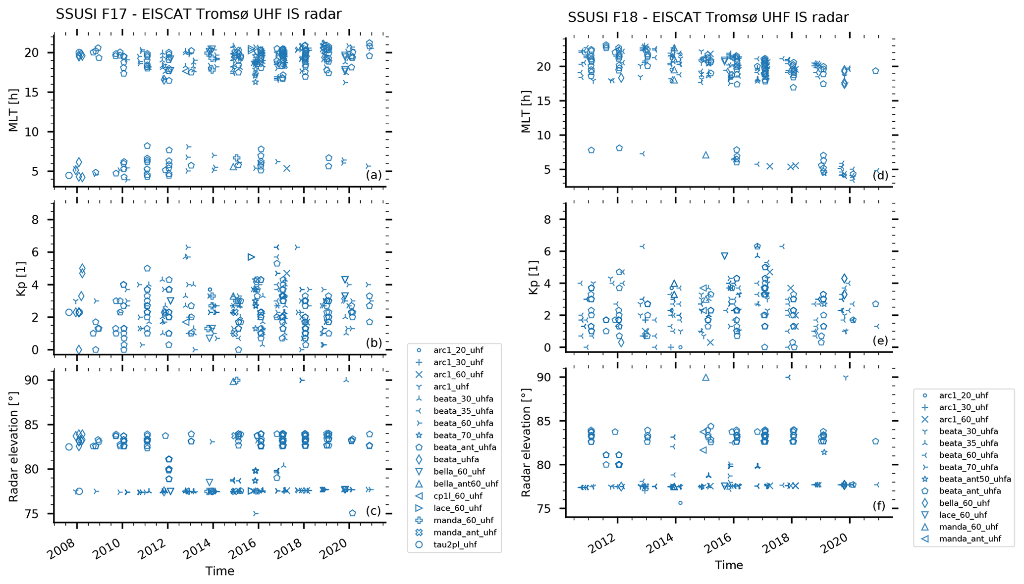
Figure 1Available coincident data between the Tromsø UHF radar and the SSUSI on DMSP/F17 (a–c) and DMSP/F18 (d–f). Shown are the distributions of the data used in the comparisons according to their magnetic local times (MLT, a, d), the geomagnetic Kp index (b, e), and the radar elevation angles (c, f). The symbols indicate the different EISCAT experiments; the ones with “ant” indicate scanning experiments following the antenna. The MLT are divided according to the times given in the text.
Table 1Number of coincidences of F17 and F18 with the EISCAT Tromsø UHF radar during the two MLT sectors.
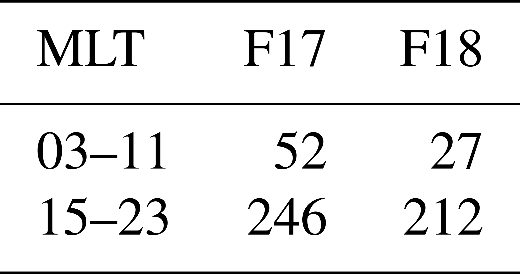
The number of coincidences used in this study is summarized in Table 1. Note that there is an asymmetry between the data available for early and late MLT, with more coincidences during the latter. This imbalance, and possibly different precipitation characteristics during the different MLT, could lead to a possible bias in the calculated electron densities and their differences to the EISCAT measurements.
4.2 Profile comparisons
As a measure of the distribution of the absolute and relative differences, we use the median together with the 68 % (≈1σ) and 95 % (≈2σ) confidence intervals derived from the 16th and 84th as well as the 2.5th and 97.5th percentiles, respectively. This enables us to quantify the differences better in cases where the distribution of those is skewed.
MLT 03–11
For early MLT (03:00–11:00 MLT), the electron density profiles together with the absolute and relative differences between the SSUSI-derived electron densities and the EISCAT Tromsø UHF radar measurements are shown in Figs. 2 and 3. The profiles were calculated over all coincidences described in Sect. 3.3, using the “standard” parameters for the ionization rates as described in Sect. 3.1 and the “aurora” recombination rate parametrization from Gledhill (1986); see Eq. (3) therein or Eq. (5) above.
The F17 morning sector results show low absolute and relative differences that grow as one approaches the peak electron density. On the other hand, F18 shows a small and nearly constant absolute difference throughout the altitude range. In both cases, the relative differences become large below the peak due to the decreasing mean electron density (the denominator in Eq. 7).
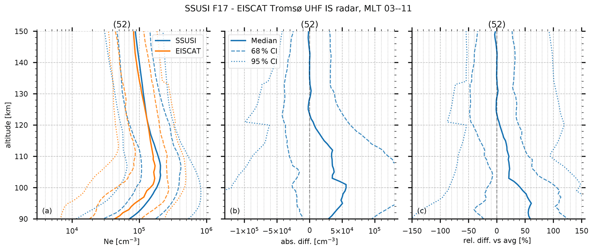
Figure 2Profile comparison of calculated electron densities from SSUSI on DMSP/F17 to the ones measured by the EISCAT Tromsø UHF radar for early MLT (03:00–11:00 MLT). Density profiles (a), absolute differences (b), and relative differences (c). Shown are the medians (solid lines) and the 68 % (dashed) and 95 % (dotted) confidence intervals for the SSUSI-calculated electron densities (blue) and EISCAT (orange). The numbers in parentheses indicate the number of coincident satellite orbits used for averaging. The SSUSI profiles have been calculated assuming a Maxwellian electron spectrum with and 35 eV per ion pair. Note that the density profiles (a) are on a logarithmic scale.
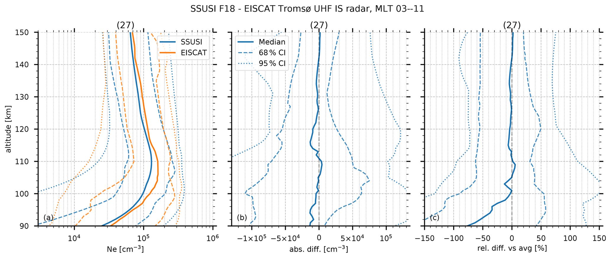
Figure 3Profile comparison as in Fig. 2 for SSUSI on DMSP/F18 and the EISCAT Tromsø UHF radar for early MLT (03:00–11:00 MLT).
For F17 (Fig. 2), the median of the absolute differences grows from near zero above 120 km to about 6×104 cm−3 (40 %) at 100 km near the peak electron density. Below the peak, the absolute differences decrease to 3×104 cm−3 near 90 km, but the relative differences increase due to the rapidly decreasing mean density. For F18 (Fig. 3), the median of the absolute differences remains between −0.5 and cm−3 above the electron density peak near 100 km, leading to relative differences between ±10 %. Below the peak, absolute differences become cm−3 at 90 km, and the magnitude of the relative differences again increases due to decreasing mean densities.
MLT 15–23
For late MLT (15:00–23:00 MLT), the electron density profiles and the absolute and relative differences between the SSUSI-derived electron densities and the EISCAT Tromsø UHF radar measurements are shown in Figs. 4 and 5. As for early MLT, the profiles were calculated over all coincidences but using a Gaussian electron spectrum and slightly larger energy per ionization event as described in Sect. 3.1.
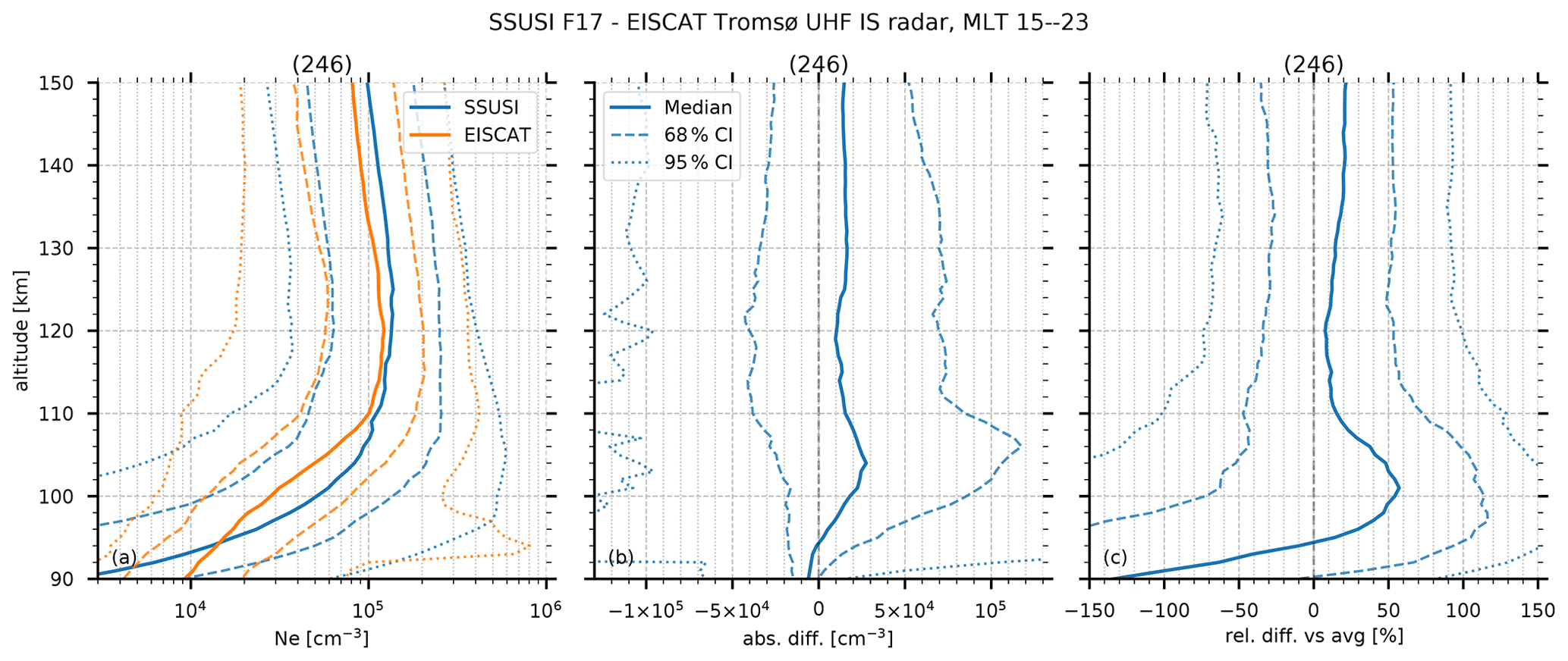
Figure 4Profile comparison as in Fig. 2 for SSUSI on DMSP/F17 and the EISCAT Tromsø UHF radar for late MLT (15:00–23:00 MLT). The SSUSI profiles have been calculated assuming a Gaussian electron spectrum with and 43.73 eV per ion pair; details can be found in the text.
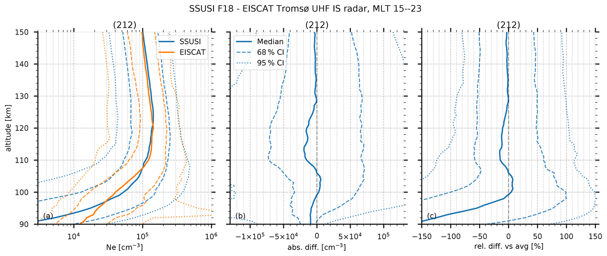
Figure 5Profile comparison as in Fig. 4 for SSUSI on DMSP/F18 and the EISCAT Tromsø UHF radar for late MLT (15:00–23:00 MLT).
For the evening sector, both the SSUSI and EISCAT observations suggest a broader electron density peak than in the morning sector. Both F17 and F18 demonstrate small and nearly constant absolute differences with EISCAT over the entire altitude range. The dipole structure of the differences would indicate a systematically higher peak height for EISCAT relative to SSUSI, and once again, the relative differences grow below the peak due to the rapidly decreasing electron density.
For F17 (Fig. 4), the median of the absolute differences is nearly constant at about 1×104 cm−3 above 125 km (15 %–20 %) and reaches 3×104 cm−3 at 105 km (50 %). While absolute differences decrease to about 0.5×104 cm−3 at 90 km, relative differences again become large due to decreasing mean densities. For F18 (Fig. 5), both absolute and relative differences are nearly zero above 125 km. However, they reach cm−3 (−15 %) at 115 km and 5×103 cm−3 (10 %) at 105 km. The absolute differences then decrease to cm−3 at 90 km, again with large relative differences.
In this study, we have used the mono-energetic approach derived by Fang et al. (2010) for atmospheric electron ionization rates and integrated over Maxwellian and Gaussian particle spectra. Related parametrizations derived explicitly for Maxwellian particle flux spectra are available (Roble and Ridley, 1987; Fang et al., 2008), and the results for those are very close to the Maxwellian case studied here (not shown). Similarly, a variety of parametrizations exists for recombination rates, and here we chose the one given in Gledhill (1986). It should be noted that the parametrization by Vickrey et al. (1982) is very similar in the altitude region used in this study, resulting in comparable results.
The results show that the approach we have presented here, which mirrors an earlier study by Aksnes et al. (2006), leads to electron densities that agree with those measured by the ground-based EISCAT radars within the variability of the data. While more sophisticated approaches may lead to closer agreement between the different techniques, they are beyond the scope of this study. Such approaches would include calculating the ionization rates by solving a transport equation as in Basu et al. (1993) or using a fully relativistic approach (Wissing and Kallenrode, 2009). Both could help to improve the ionization rate profiles and the backscatter ratio of the electrons. They would also enable different pitch-angle distributions to be used instead of relying on isotropic flux as in this study.
The differences observed between the different MLT sectors may be the result of different precipitation characteristics during the different times (Rees, 1969). Different magnetospheric acceleration mechanisms influence these characteristics; a short summary about the general mechanisms can be found, for example, in Khazanov and Chen (2021). The observed emissions usually result from a mixture of these different auroral cases, and it seems that in our case, more backscattering occurs during the evening MLT than during the morning MLT measurements. One should note that the evening MLT corresponds to the beginning of the night, and the auroral emissions just start to occur. In addition, the exact amount of backscattering has been a debate for decades, ranging from 17 % (Rees, 1963) to close to 50 % (Banks et al., 1974), to presumably even higher values depending on the incident energy (Khazanov and Chen, 2021).
Note that the energy range provided by the SSUSI Auroral-EDR data is limited to 2–20 keV, which also limits the altitude range of comparable ionization rates to approximately 90–150 km (e.g Fang et al., 2008, 2010). The increasing (negative) differences between the SSUSI results and EISCAT at lower altitudes thus indicate the limits of the unambiguous energy range for the FUV-derived electron characteristics as described in Sect. 2.1.
It should be noted that the average energy and energy flux derived from the LBH emissions are essentially moments of the true distribution, such that one way to mitigate this problem may be assuming a different spectrum, for example, by adding a high-energy tail to the Maxwellian or Gaussian spectra (e.g. Strickland et al., 1993). However, the SSUSI energy range is typical for auroral inputs, and good results at lower altitudes are not expected without further assumptions about the electron spectra. In addition, at lower altitudes the recombination rates increase substantially (Gledhill, 1986). This leads to increasing difficulties at lower altitudes when comparing observations of dynamic aurora by instruments with different observing volumes and spatio-temporal samplings as is the case here; the SSUSI instruments image a large area around the radar, while the EISCAT is a narrow beam. Thus, future studies may employ ion-chemistry models such as the Sodankylä Ion Chemistry (SIC) model (Verronen et al., 2005; Turunen et al., 2009) to improve upon the recombination and quenching rates. Those models may also be used to derive trace-gas species directly, which opens up even more possibilities of comparisons, for example, against satellite-based and ground-based trace-gas measurements.
In this study we validate the electron density profiles derived from the SSUSI data products for effective energy and flux by comparing them to EISCAT-derived electron density profiles. This comparison shows that SSUSI FUV observations can be used to provide high-resolution (down to 10 km × 10 km) ionization rate profiles across its 3000 km wide swath within the auroral zone that are comparable to those measured by EISCAT between 100 and 150 km. In principle, the ionization rates can then also be used to calculate E-region conductivity and trace-gas profiles.
The data indicate that the comparison between the SSUSI volume measurements and the EISCAT narrow beam observations within that volume results in considerable pass-to-pass variability of the differences, caused by the wide range of auroral conditions and different precipitation characteristics. As a result, there are no statistically significant differences between the two measurement techniques. However, the trends in the comparisons show that a Maxwellian distribution with an energy loss per electron–ion pair of 35 eV is adequate for the morning sector (03:00–11:00 MLT). On the other hand, in the evening sector (15:00–23:00 MLT), where more backscattered electrons are present, a Gaussian distribution with an energy loss of 43.73 eV per electron–ion pair is required to duplicate the higher and broader electron density peak.
The results show that electron densities derived from both SSUSI F17 and F18 agree with those measured by EISCAT to within 0 %–20 % above 120 km. Although the differences are not statistically significant, the trend in the biases indicates that the SSUSI estimates are generally higher, and the differences are larger for the evening sector in comparison to the morning sector. While SSUSI F18 maintains small, ≈10 % differences with EISCAT through the peak of the electron density profile near 100 km, the trend of the SSUSI F17 bias tends to increase towards the peak, reaching as high as 40 % before decreasing.
Below the peak density, the relative differences between EISCAT and both satellites become large due to the rapidly decreasing electron density. In addition, the SSUSI results tend to be smaller than the EISCAT densities below 95 km, indicating that the Maxwellian and Gaussian spectra may lack the high energies required to create ionization in this region. While the bias is not significant, the tendency for SSUSI to underestimate the electron density at lower altitudes may be the result of the 20 keV limit of the SSUSI energy retrievals. This bias may also be due to the short recombination times in this region shortening the coherence times between the observations and the parametrization failing to account for the formation of negative ions.
In virtually all cases (early and late MLT), the differences between EISCAT- and SSUSI-derived electron densities are well within the 68 % (≈1σ) confidence interval derived from the distribution of the differences and are always less than 2σ. Thus, the SSUSI instrument may be used to extend the EISCAT measurements across the auroral zone, quantifying both the auroral energy deposition and its spatial variability. Based on this work, future studies can further adjust the spectra as well as the recombination and quenching rates used for converting the UV emissions to electron energies and fluxes to match the ground-based measurements even better.
The SSUSI data used in this study are available at https://ssusi.jhuapl.edu/data_products (last access: 21 September 2020) (SSUSI, 2020), and the EISCAT data are available via the “Madrigal” database http://cedar.openmadrigal.org (last access: 21 September 2020) (EISCAT, 2020). The source code used to calculate the ionization rates and electron densities is available at https://doi.org/10.5281/zenodo.4298137 (Bender, 2020) or upon request from the first author.
SB carried out the data analysis and set up the manuscript. PJE and LJP contributed to the discussion and use of language. All authors contributed to the interpretation and discussion of the method and the results as well as to the writing of the manuscript.
The authors declare that they have no conflict of interest.
Publisher's note: Copernicus Publications remains neutral with regard to jurisdictional claims in published maps and institutional affiliations.
Stefan Bender and Patrick J. Espy acknowledge support from the Birkeland Center for Space Sciences (BCSS), supported by the Research Council of Norway under grant no. 223252/F50. Larry J. Paxton is the principal investigator of the SSUSI project. EISCAT is an international association supported by research organizations in China (CRIRP), Finland (SA), Japan (NIPR and ISEE), Norway (NFR), Sweden (VR), and the United Kingdom (UKRI). The computations were performed on resources provided by UNINETT Sigma2 – the National Infrastructure for High Performance Computing and Data Storage in Norway. We further acknowledge the contributions by Harold K. Knight to the discussion.
This research has been supported by the Norges Forskningsråd (grant no. 223252/F50).
This paper was edited by Dalia Buresova and reviewed by two anonymous referees.
Ajello, J. M., Evans, J. S., Veibell, V., Malone, C. P., Holsclaw, G. M., Hoskins, A. C., Lee, R. A., McClintock, W. E., Aryal, S., Eastes, R. W., and Schneider, N.: The UV Spectrum of the Lyman–Birge–Hopfield Band System of N2 Induced by Cascading from Electron Impact, J. Geophys. Res.-Space, 125, e2019JA027546, https://doi.org/10.1029/2019ja027546, 2020. a
Aksnes, A., Stadsnes, J., Østgaard, N., Germany, G. A., Oksavik, K., Vondrak, R. R., Brekke, A., and Løvhaug, U. P.: Height profiles of the ionospheric electron density derived using space-based remote sensing of UV and X ray emissions and EISCAT radar data: A ground-truth experiment, J. Geophys. Res.-Space, 111, A02 301, https://doi.org/10.1029/2005ja011331, 2006. a, b, c, d, e, f, g
Banks, P. M., Chappell, C. R., and Nagy, A. F.: A new model for the interaction of auroral electrons with the atmosphere: Spectral degradation, backscatter, optical emission, and ionization, J. Geophys. Res., 79, 1459–1470, https://doi.org/10.1029/ja079i010p01459, 1974. a, b, c
Basu, B., Jasperse, J. R., Strickland, D. J., and Daniell, R. E.: Transport-Theoretic Model for the Electron-Proton-Hydrogen Atom Aurora, 1. Theory, J. Geophys. Res.-Space, 98, 21517–21532, https://doi.org/10.1029/93ja01646, 1993. a, b, c, d, e
Bender, S.: st-bender/pyeppaurora: Version 0.0.5, Zenodo [code], https://doi.org/10.5281/zenodo.4298137, 2020. a
Brasseur, G. P. and Solomon, S.: Aeronomy of the Middle Atmosphere, Atmospheric and Oceanographic Sciences Library, 32, Springer-Verlag, Dordrecht, the Netherlands, https://doi.org/10.1007/1-4020-3824-0, 2005. a
Dupuy, E., Walker, K. A., Kar, J., Boone, C. D., McElroy, C. T., Bernath, P. F., Drummond, J. R., Skelton, R., McLeod, S. D., Hughes, R. C., Nowlan, C. R., Dufour, D. G., Zou, J., Nichitiu, F., Strong, K., Baron, P., Bevilacqua, R. M., Blumenstock, T., Bodeker, G. E., Borsdorff, T., Bourassa, A. E., Bovensmann, H., Boyd, I. S., Bracher, A., Brogniez, C., Burrows, J. P., Catoire, V., Ceccherini, S., Chabrillat, S., Christensen, T., Coffey, M. T., Cortesi, U., Davies, J., De Clercq, C., Degenstein, D. A., De Mazière, M., Demoulin, P., Dodion, J., Firanski, B., Fischer, H., Forbes, G., Froidevaux, L., Fussen, D., Gerard, P., Godin-Beekmann, S., Goutail, F., Granville, J., Griffith, D., Haley, C. S., Hannigan, J. W., Höpfner, M., Jin, J. J., Jones, A., Jones, N. B., Jucks, K., Kagawa, A., Kasai, Y., Kerzenmacher, T. E., Kleinböhl, A., Klekociuk, A. R., Kramer, I., Küllmann, H., Kuttippurath, J., Kyrölä, E., Lambert, J.-C., Livesey, N. J., Llewellyn, E. J., Lloyd, N. D., Mahieu, E., Manney, G. L., Marshall, B. T., McConnell, J. C., McCormick, M. P., McDermid, I. S., McHugh, M., McLinden, C. A., Mellqvist, J., Mizutani, K., Murayama, Y., Murtagh, D. P., Oelhaf, H., Parrish, A., Petelina, S. V., Piccolo, C., Pommereau, J.-P., Randall, C. E., Robert, C., Roth, C., Schneider, M., Senten, C., Steck, T., Strandberg, A., Strawbridge, K. B., Sussmann, R., Swart, D. P. J., Tarasick, D. W., Taylor, J. R., Tétard, C., Thomason, L. W., Thompson, A. M., Tully, M. B., Urban, J., Vanhellemont, F., Vigouroux, C., von Clarmann, T., von der Gathen, P., von Savigny, C., Waters, J. W., Witte, J. C., Wolff, M., and Zawodny, J. M.: Validation of ozone measurements from the Atmospheric Chemistry Experiment (ACE), Atmos. Chem. Phys., 9, 287–343, https://doi.org/10.5194/acp-9-287-2009, 2009. a, b
EISCAT: CEDAR Madrigal Database, available at: http://cedar.openmadrigal.org, last access: 21 September 2020. a
Fang, X., Randall, C. E., Lummerzheim, D., Solomon, S. C., Mills, M. J., Marsh, D. R., Jackman, C. H., Wang, W., and Lu, G.: Electron impact ionization: A new parameterization for 100 eV to 1 MeV electrons, J. Geophys. Res.-Space, 113, A09311, https://doi.org/10.1029/2008ja013384, 2008. a, b, c, d
Fang, X., Randall, C. E., Lummerzheim, D., Wang, W., Lu, G., Solomon, S. C., and Frahm, R. A.: Parameterization of monoenergetic electron impact ionization, Geophys. Res. Lett., 37, L22 106, https://doi.org/10.1029/2010gl045406, 2010. a, b, c, d, e, f, g, h, i
Funke, B., López-Puertas, M., Gil-López, S., von Clarmann, T., Stiller, G. P., Fischer, H., and Kellmann, S.: Downward transport of upper atmospheric NOx into the polar stratosphere and lower mesosphere during the Antarctic 2003 and Arctic 2002/2003 winters, J. Geophys. Res.-Atmos., 110, D24 308, https://doi.org/10.1029/2005JD006463, 2005. a
Funke, B., Ball, W., Bender, S., Gardini, A., Harvey, V. L., Lambert, A., López-Puertas, M., Marsh, D. R., Meraner, K., Nieder, H., Päivärinta, S.-M., Pérot, K., Randall, C. E., Reddmann, T., Rozanov, E., Schmidt, H., Seppälä, A., Sinnhuber, M., Sukhodolov, T., Stiller, G. P., Tsvetkova, N. D., Verronen, P. T., Versick, S., von Clarmann, T., Walker, K. A., and Yushkov, V.: HEPPA-II model–measurement intercomparison project: EPP indirect effects during the dynamically perturbed NH winter 2008–2009, Atmos. Chem. Phys., 17, 3573–3604, https://doi.org/10.5194/acp-17-3573-2017, 2017. a
Germany, G. A., Torr, M. R., Richards, P. G., and Torr, D. G.: The dependence of modeled OI 1356 and N2 Lyman Birge Hopfield auroral emissions on the neutral atmosphere, J. Geophys. Res.-Space, 95, 7725, https://doi.org/10.1029/ja095ia06p07725, 1990. a, b
Gledhill, J. A.: The effective recombination coefficient of electrons in the ionosphere between 50 and 150 km, Radio Sci., 21, 399–408, https://doi.org/10.1029/rs021i003p00399, 1986. a, b, c, d, e, f, g, h
Khazanov, G. V. and Chen, M. W.: Why Atmospheric Backscatter Is Important in the Formation of Electron Precipitation in the Diffuse Aurora, J. Geophys. Res.-Space, 126, e2021JA029211, https://doi.org/10.1029/2021ja029211, 2021. a, b, c
Knight, H. K.: Auroral ionospheric E region parameters obtained from satellite- based far-ultraviolet and ground-based ionosonde observations – effects of proton precipitation, Ann. Geophys., 39, 105–118, https://doi.org/10.5194/angeo-39-105-2021, 2021. a
Knight, H. K., Galkin, I. A., Reinisch, B. W., and Zhang, Y.: Auroral Ionospheric E Region Parameters Obtained From Satellite-Based Far Ultraviolet and Ground-Based Ionosonde Observations: Data, Methods, and Comparisons, J. Geophys. Res.-Space, 123, 6065–6089, https://doi.org/10.1029/2017ja024822, https://doi.org/10.1029/2017JA024822, 2018. a, b, c, d
Lehtinen, M. S. and Huuskonen, A.: General incoherent scatter analysis and GUISDAP, J. Atmos. Terr. Phys., 58, 435–452, https://doi.org/10.1016/0021-9169(95)00047-x, 1996. a
Lossow, S., Khosrawi, F., Kiefer, M., Walker, K. A., Bertaux, J.-L., Blanot, L., Russell, J. M., Remsberg, E. E., Gille, J. C., Sugita, T., Sioris, C. E., Dinelli, B. M., Papandrea, E., Raspollini, P., García-Comas, M., Stiller, G. P., von Clarmann, T., Dudhia, A., Read, W. G., Nedoluha, G. E., Damadeo, R. P., Zawodny, J. M., Weigel, K., Rozanov, A., Azam, F., Bramstedt, K., Noël, S., Burrows, J. P., Sagawa, H., Kasai, Y., Urban, J., Eriksson, P., Murtagh, D. P., Hervig, M. E., Högberg, C., Hurst, D. F., and Rosenlof, K. H.: The SPARC water vapour assessment II: profile-to-profile comparisons of stratospheric and lower mesospheric water vapour data sets obtained from satellites, Atmos. Meas. Tech., 12, 2693–2732, https://doi.org/10.5194/amt-12-2693-2019, 2019. a, b
Matthes, K., Funke, B., Andersson, M. E., Barnard, L., Beer, J., Charbonneau, P., Clilverd, M. A., Dudok de Wit, T., Haberreiter, M., Hendry, A., Jackman, C. H., Kretzschmar, M., Kruschke, T., Kunze, M., Langematz, U., Marsh, D. R., Maycock, A. C., Misios, S., Rodger, C. J., Scaife, A. A., Seppälä, A., Shangguan, M., Sinnhuber, M., Tourpali, K., Usoskin, I., van de Kamp, M., Verronen, P. T., and Versick, S.: Solar forcing for CMIP6 (v3.2), Geosci. Model Dev., 10, 2247–2302, https://doi.org/10.5194/gmd-10-2247-2017, 2017. a
Paxton, L. J. and Zhang, Y.: Space Weather Fundamentals, chap. Far ultraviolet imaging of the aurora, 213–244, CRC Press Laurel, MD, USA, 2016. a
Paxton, L. J., Meng, C.-I., Fountain, G. H., Ogorzalek, B. S., Darlington, E. H., Gary, S. A., Goldsten, J. O., Kusnierkiewicz, D. Y., Lee, S. C., Linstrom, L. A., Maynard, J. J., Peacock, K., Persons, D. F., and Smith, B. E.: Special sensor ultraviolet spectrographic imager: an instrument description, in: Instrumentation for Planetary and Terrestrial Atmospheric Remote Sensing, edited by: Chakrabarti, S. and Christensen, A. B., SPIE, https://doi.org/10.1117/12.60595, 1992. a, b, c, d
Paxton, L. J., Meng, C.-I., Fountain, G. H., Ogorzalek, B. S., Darlington, E. H., Gary, S. A., Goldsten, J. O., Kusnierkiewicz, D. Y., Lee, S. C., Linstrom, L. A., Maynard, J. J., Peacock, K., Persons, D. F., Smith, B. E., Strickland, D. J., and Daniell Jr., R. E.: SSUSI – Horizon-to-horizon and limb-viewing spectrographic imager for remote sensing of environmental parameters, in: Ultraviolet Technology IV, edited by: Huffman, R. E., SPIE, https://doi.org/10.1117/12.140846, 1993. a, b, c, d
Paxton, L. J., Morrison, D., Zhang, Y., Kil, H., Wolven, B., Ogorzalek, B. S., Humm, D. C., and Meng, C.-I.: Validation of remote sensing products produced by the Special Sensor Ultraviolet Scanning Imager (SSUSI): a far UV-imaging spectrograph on DMSP F-16, in: Optical Spectroscopic Techniques, Remote Sensing, and Instrumentation for Atmospheric and Space Research IV, edited by: Larar, A. M. and Mlynczak, M. G., SPIE, https://doi.org/10.1117/12.454268, 2002. a
Paxton, L. J., Schaefer, R. K., Zhang, Y., and Kil, H.: Far ultraviolet instrument technology, J. Geophys. Res.-Space, 122, 2706–2733, https://doi.org/10.1002/2016ja023578, 2017. a, b, c, d
Paxton, L. J., Schaefer, R. K., Zhang, Y., Kil, H., and Hicks, J. E.: SSUSI and SSUSI-Lite: Providing Space Situational Awareness and Support for Over 25 Years, Johns Hopkins APL Tech. D., 34, 388–400, 2018. a
Picone, J. M., Hedin, A. E., Drob, D. P., and Aikin, A. C.: NRLMSISE-00 empirical model of the atmosphere: Statistical comparisons and scientific issues, J. Geophys. Res.-Space, 107, 1468, https://doi.org/10.1029/2002JA009430, 2002. a
Porter, H. S., Jackman, C. H., and Green, A. E. S.: Efficiencies for production of atomic nitrogen and oxygen by relativistic proton impact in air, J. Chem. Phys., 65, 154–167, https://doi.org/10.1063/1.432812, 1976. a
Randall, C. E.: Validation of POAM III ozone: Comparisons with ozonesonde and satellite data, J. Geophys. Res.-Atmos., 108, 4367, https://doi.org/10.1029/2002jd002944, 2003. a
Randall, C. E.: Stratospheric effects of energetic particle precipitation in 2003–2004, Geophys. Res. Lett., 32, L05 802, https://doi.org/10.1029/2004gl022003, 2005. a
Randall, C. E., Siskind, D. E., and Bevilacqua, R. M.: Stratospheric NOx enhancements in the Southern Hemisphere Vortex in winter/spring of 2000, Geophys. Res. Lett., 28, 2385–2388, https://doi.org/10.1029/2000gl012746, 2001. a
Randall, C. E., Harvey, V. L., Siskind, D. E., France, J., Bernath, P. F., Boone, C. D., and Walker, K. A.: NOx descent in the Arctic middle atmosphere in early 2009, Geophys. Res. Lett., 36, L18811, https://doi.org/10.1029/2009GL039706, 2009. a, b, c
Rees, M.: Auroral electrons, Space Sci. Rev., 10, 413–441, https://doi.org/10.1007/bf00203621, 1969. a
Rees, M. H.: Auroral ionization and excitation by incident energetic electrons, Planet. Space Sci., 11, 1209–1218, https://doi.org/10.1016/0032-0633(63)90252-6, 1963. a, b, c
Robinson, R. M. and Vondrak, R. R.: Validation of techniques for space based remote sensing of auroral precipitation and its ionospheric effects, Space Sci. Rev., 69, 331–407, https://doi.org/10.1007/bf02101699, 1994. a, b, c
Roble, R. G. and Ridley, E. C.: An auroral model for the NCAR thermospheric general circulation model (TGCM), Ann. Geophys., 5, 369–382, 1987. a, b, c
Schröter, J., Heber, B., Steinhilber, F., and Kallenrode, M.: Energetic particles in the atmosphere: A Monte-carlo simulation, Adv. Space Res., 37, 1597–1601, https://doi.org/10.1016/j.asr.2005.05.085, 2006. a
Smith-Johnsen, C., Marsh, D. R., Orsolini, Y., Tyssøy, H. N., Hendrickx, K., Sandanger, M. I., Ødegaard, L.-K. G., and Stordal, F.: Nitric Oxide Response to the April 2010 Electron Precipitation Event: Using WACCM and WACCM-D With and Without Medium-Energy Electrons, J. Geophys. Res.-Space, 123, 5232–5245, https://doi.org/10.1029/2018ja025418, 2018. a, b
SSUSI: Data Products, available at: https://ssusi.jhuapl.edu/data_products, last access: 21 September 2020. a
Strickland, D., Bishop, J., Evans, J., Majeed, T., Shen, P., Cox, R., Link, R., and Huffman, R.: Atmospheric Ultraviolet Radiance Integrated Code (AURIC): theory, software architecture, inputs, and selected results, J. Quant. Spectrosc. Ra., 62, 689–742, https://doi.org/10.1016/s0022-4073(98)00098-3, 1999. a, b, c
Strickland, D. J., Jasperse, J. R., and Whalen, J. A.: Dependence of auroral FUV emissions on the incident electron spectrum and neutral atmosphere, J. Geophys. Res.-Space, 88, 8051, https://doi.org/10.1029/ja088ia10p08051, 1983. a, b, c
Strickland, D. J., Daniell, R. E., Jasperse, J. R., and Basu, B.: Transport-Theoretic Model for the Electron–Proton–Hydrogen Atom Aurora, 2. Model Results, J. Geophys. Res.-Space, 98, 21533–21548, https://doi.org/10.1029/93ja01645, 1993. a, b, c, d, e, f
Strong, K., Wolff, M. A., Kerzenmacher, T. E., Walker, K. A., Bernath, P. F., Blumenstock, T., Boone, C., Catoire, V., Coffey, M., De Mazière, M., Demoulin, P., Duchatelet, P., Dupuy, E., Hannigan, J., Höpfner, M., Glatthor, N., Griffith, D. W. T., Jin, J. J., Jones, N., Jucks, K., Kuellmann, H., Kuttippurath, J., Lambert, A., Mahieu, E., McConnell, J. C., Mellqvist, J., Mikuteit, S., Murtagh, D. P., Notholt, J., Piccolo, C., Raspollini, P., Ridolfi, M., Robert, C., Schneider, M., Schrems, O., Semeniuk, K., Senten, C., Stiller, G. P., Strandberg, A., Taylor, J., Tétard, C., Toohey, M., Urban, J., Warneke, T., and Wood, S.: Validation of ACE-FTS N2O measurements, Atmos. Chem. Phys., 8, 4759–4786, https://doi.org/10.5194/acp-8-4759-2008, 2008. a
Torr, M. R., Torr, D. G., Zukic, M., Johnson, R. B., Ajello, J., Banks, P., Clark, K., Cole, K., Keffer, C., Parks, G., Tsurutani, B., and Spann, J.: A far ultraviolet imager for the International Solar-Terrestrial Physics Mission, Space Sci. Rev., 71, 329–383, https://doi.org/10.1007/bf00751335, 1995. a
Turunen, E., Verronen, P. T., Seppälä, A., Rodger, C. J., Clilverd, M. A., Tamminen, J., Enell, C.-F., and Ulich, T.: Impact of different energies of precipitating particles on NOx generation in the middle and upper atmosphere during geomagnetic storms, J. Atmos. Sol.-Terr. Phy., 71, 1176–1189, https://doi.org/10.1016/j.jastp.2008.07.005, 2009. a
van de Kamp, M., Seppälä, A., Clilverd, M. A., Rodger, C. J., Verronen, P. T., and Whittaker, I. C.: A model providing long-term data sets of energetic electron precipitation during geomagnetic storms, J. Geophys. Res.-Atmos., 121, 12520–12540, https://doi.org/10.1002/2015jd024212, 2016. a
Verronen, P. T., Seppälä, A., Clilverd, M. A., Rodger, C. J., Kyrölä, E., Enell, C.-F., Ulich, T., and Turunen, E.: Diurnal variation of ozone depletion during the October–November 2003 solar proton events, J. Geophys. Res.-Space, 110, A09S32, https://doi.org/10.1029/2004ja010932, 2005. a
Vickrey, J. F., Vondrak, R. R., and Matthews, S. J.: Energy deposition by precipitating particles and Joule dissipation in the auroral ionosphere, J. Geophys. Res.-Space, 87, 5184–5196, https://doi.org/10.1029/ja087ia07p05184, 1982. a, b, c
Vondrak, R. R. and Baron, M. J.: Radar measurements of the latitudinal variation of auroral ionization, Radio Sci., 11, 939–946, https://doi.org/10.1029/rs011i011p00939, 1976. a, b, c, d
Wissing, J. M. and Kallenrode, M.-B.: Atmospheric Ionization Module Osnabrück (AIMOS): A 3-D model to determine atmospheric ionization by energetic charged particles from different populations, J. Geophys. Res.-Space, 114, A06 104, https://doi.org/10.1029/2008ja013884, 2009. a, b, c
Let A be the set of all SSUSI points within the comparison area, and B the set of valid points, i.e. the points used for the profile calculation defined by Then, the scaling we apply is equal to , with the flux given in the SSUSI data files and the cardinality of the sets.