the Creative Commons Attribution 4.0 License.
the Creative Commons Attribution 4.0 License.
 | 20 Aug 2021
Climatology of ionosphere over Nepal based on GPS total electron content data from 2008 to 2018
Drabindra Pandit
Basudev Ghimire
Christine Amory-Mazaudier
Rolland Fleury
Narayan Prasad Chapagain
Binod Adhikari
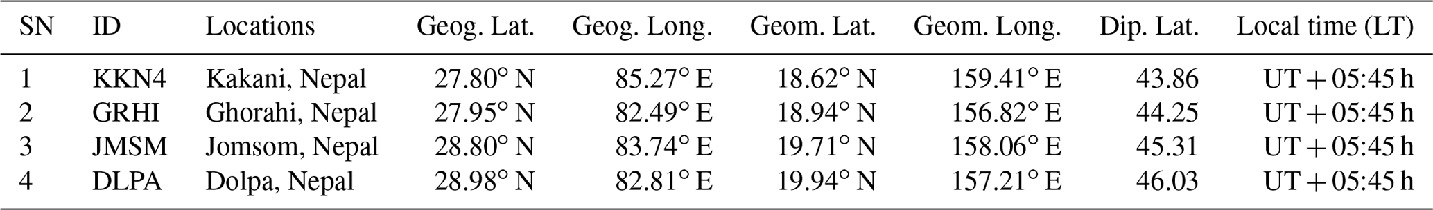
In this study, we analyse the climatology of ionosphere over Nepal based on GPS-derived vertical total electron content (VTEC) observed from four stations as defined in Table 1: KKN4 (27.80∘ N, 85.27∘ E), GRHI (27.95∘ N, 82.49∘ E), JMSM (28.80∘ N, 83.74∘ E) and DLPA (28.98∘ N, 82.81∘ E) during the years 2008 to 2018. The study illustrates the diurnal, monthly, annual, seasonal and solar cycle variations in VTEC during all times of solar cycle 24. The results clearly reveal the presence of equinoctial asymmetry in TEC, which is more pronounced in maximum phases of solar cycle in the year 2014 at KKN4 station, followed by descending, ascending and minimum phases. Diurnal variations in VTEC showed the short-lived day minimum which occurs between 05:00 to 06:00 LT (local time) at all the stations considered, with diurnal peaks between 12:00 and 15:00 LT. The maximum value of TEC is observed more often during the spring equinox than the autumn equinox, with a few asymmetries. Seasonal variation in TEC is observed to be a manifestation of variations in solar flux, particularly regarding the level of solar flux in consecutive solstices.
- Article
(1979 KB) - Full-text XML
- BibTeX
- EndNote


Total electron content (TEC) is a crucial parameter of ionosphere comprising high concentrations of electrons and ions formed under the ionization of extreme ultraviolet (EUV) radiation and solar X-rays. The lower atmospheric disturbance also contributes to ionospheric variability (Anderson and Fuller-Rowell, 1999; Prikryal et al., 2010). Numerous periodic and aperiodic variabilities identified in the ionosphere make the impact on the applications involving the radio link between satellites and the ground, which plays vital role in the communication, navigation and surveillance, with important consequences for the reliability and accuracy of the service (Guo et al., 2015). The global positioning system (GPS) is widely used in recent appliances which encounter the largest errors in the path due to disturbed ionospheric free electrons, emphasizing the need to study GPS–TEC variability. The application of GPS technology gives scientists insight into the shape and behaviour of the ionosphere. A list of factors affecting TEC includes ionospheric electron density, ion–electron temperature, composition, dynamic variations with altitude, latitude, longitude, local time, seasons, solar and magnetic activity. Because the equatorial ionosphere is highly vulnerable, it poses major threats to communication signals. The ionosphere at the mid latitude is less variable; hence, most of the observations and measurements are taken from this region, whereas the high latitude ionosphere is sensitive to outer space as it is connected by geomagnetic field lines (Akala et al., 2013; Parwani et al., 2019). The study of VTEC at the low–mid ionosphere showed solar activity dependence (Shimeis et al., 2014). TEC has been studied by a large number of researchers; Rama Rao et al. (1980) studied the diurnal variation in TEC at Waltair, India, and found a short-lived predawn minimum, a steep early morning rise followed by broad mid-afternoon maximum and a steep post-sunset fall. The relation between TEC and the sunspot number (SSN), F10.7 and EUV was studied by Dabaset al. (1993), who pointed out that TEC has a nonlinear relation with SSN and a linear relation with F10.7 and EUV. Ouattara and Amory-Mazaudier (2012) showed the impact of solar activity on diurnal variability during different phases of the solar cycle. An analogous study was carried out around the globe using various methods of TEC, such as diurnal, monthly, seasonal and solar cycle and solar activity dependency, e.g. in South Asia (Chauhan et al., 2011; Walker et al., 1994), in South America (Sahai et al., 2007; Natali and Meza, 2011; Akala et al., 2013; de Abreu et al., 2014), over North America (Huo et al., 2009; Perevalova et al., 2010), in Africa (Shimeis et al., 2014; D'ujanga et al., 2012; Ouattara and Fleury, 2011; Zoundi et al., 2012), over Brazil (Venkatesh et al., 2014a, 2014b, 2015), over Japan (Zakharenkova et al., 2012; Mansoori et al., 2016) and over China (Guo et al., 2015; Zhao et al., 2007; Liu et al., 2013).
TEC studied at the Jet Propulsion Laboratory for the years 1998–2008 found stronger annual TEC variation in the Southern Hemisphere, and the variation in phase and amplitude is more in the conjugate hemisphere (Liu et al., 2009). Galav et al. (2010) found semiannual periodicity in daytime TEC, the spring equinox shows the highest TEC, and winter solstices are the lowest in India. The winter anomaly, semiannual anomaly and annual anomaly are described by Liu and Chen (2009) and Rishbeth and Garriott (1998). Global-scale TEC research found that the effect on TEC was stronger during the day than at night and also at low latitudes than at high latitudes. The effect on TEC is seen more on the either side of the magnetic equator than at the magnetic equator (Liu et al., 2009). Dashora and Suresh (2015) analysed the characteristics of low latitude TEC data of solar cycles 23 and 24 over Indian sector using global ionospheric data. A double hump structure in the solar flux and in TEC was identified at the low latitude station of Varanasi, India, in the ionospheric response using the GPS TEC, IRI (International Reference Ionosphere) and TIE-GCM (Thermosphere–Ionosphere–Electrodynamics General Circulation Model) TEC of solar cycle 24 by Rao et al. (2019a). Parwani et al. (2019) studied the latitudinal variation in ionospheric TEC in the northern hemispheric region and found that the diurnal TEC has a higher value in low latitudes than in mid and high latitudes and in the seasonal variation maximum in spring and autumn than in summer and winter.
Many studies on TEC have been conducted in Asia; however, no result for the climatology of TEC over Nepal, for a long time series, about one solar cycle has been reported up to now. In this paper, we present, for the first time, characteristics of ionosphere in Nepal, such as the diurnal, annual, seasonal and solar cycle dependence of TEC on the local ionospheric conditions, using GPS TEC data obtained from the four GPS stations of KKN4, GRHI, JMSM and DLPA (see Table 1). Our study includes GPS TEC data from 2008 to 2018 of solar cycle 24, including all four phases of this sunspot cycle, the minimum phase of the years 2008–2009, the ascending phase of the years 2010–2011, the maximum phase from 2012 to 2014 and the descending phase of years 2015–2018. The second section of this paper includes the data set and methodology, and the third includes the results and discussion. The concluding remarks are discussed in the last section.
Total electron content (TEC) is the total number of electrons integrated along the path from the receiver to each GPS satellite which orbits the Earth at an altitude of 20 200 km. It measures in TEC units (TECU), where 1 TECU=1016 electron per square metre. The TEC is obtained as follows (Hofmann-Wellenhof et al., 1992):
where Ne is electron density, R is the receiver altitude, and S is the satellite altitude. The dual frequency GPS receiver in the two L-bands of frequency f1=1575.42 MHz and f2=1227.60 MHz provide the carrier phase and pseudo-range measurements. The TEC is calculated from the L1 and L2 pseudo-range and carrier phase (Hofmann-Wellenhof et al., 1992). Using the pseudo-range and phase data, TEC is calculated as follows:
where P1 and P2 are the pseudo-ranges for frequencies f1 and f2, respectively.
The TEC obtained by this method is called slanted TEC (STEC), which is a measure of the total electron content of the ionosphere along the ray path from the satellite to receiver and has to be converted to vertical TEC (VTEC) using the equation (Titheridge, 1972).
where Bs and Bu are the biases of instruments of satellites and receivers, respectively, ε is the elevation angle of the satellite, and Re=6371 km is the mean radius of the Earth.
For this study, data were carried out with GPS data taken from four GPS stations (DLPA, JMSM, KKN4 and GRHI) from Nepal. The details of the stations, including their geographical and geomagnetic coordinates, are shown in Table 1 and universal time is used for all time references. The GPS data of the four stations were downloaded from http://www.unavco.org, last access: 15 March 2020, which is freely available to all users. These data are available in RINEX (Receiver Independent Exchange) format v2.1, which is a standard ASCII (American Standard Code for Information Interchange) format. The temporal resolution of this data is 15 min. The raw data are then processed using software developed by Rolland Fleury (Lab-STICC, UMR 6285, Institut Mines-Télécom Atlantique, site de Brest, France, 19 July 2018; available at http://www.girgea.org, last access: 19 July 2018), which runs on a Windows operating system to obtain the required TEC.
Table 1The selected GPS stations and their coordinates, the data of which are used in the study.
The data for the solar indices sunspot number (SSN) and solar flux index (F10.7) to study long term solar activity are taken from Royal Observatory of Belgium, Brussels (http://sidc.oma.be/silso/home, last access: 6 April 2020), and OMNIWeb (http://omniweb.gsfc.nasa.gov/, last access: 6 April 2020). SSN is one of the most the consistent solar indices and effectively describes solar activities, and the are valuable for forecasting space weather phenomena. The solar flux index provides the information about the total emission produced by the Sun at the wavelength of F10.7 cm to the Earth.
In this study, we use GPS-derived TEC from RINEX files, using this method to obtain TEC calibrated at 15 min for all measures. Between 30 s VTEC sequences, the elevation may vary. This leads to variation in the VTEC, depending on the constellation and not just the variation in the content over that period. We have chosen to do the regression over a period 15 min, with the VTEC obtained displayed in the middle of this period. This makes it possible to have four points over 1 h and, therefore, to have an evolution of the VTEC 4 times more precise than that of global ionosphere maps (GIMs), which are currently in time steps of 1 or 2 h, depending on the organization. So, it provides a better possibility to see and characterize finer local structures in RINEX-derived TEC than in GIMs.
Table 2Classification of selected years according to the solar cycle phases.

This study analyses variations in VTEC during different phases of solar cycle 24, along with the annual, seasonal and diurnal variations. For this, the local seasons are classified as winter (November–February), spring (March and April), summer (May–August) and autumn (September and October). The classifications of the selected years, as per solar cycle phases, are presented in Table 2.
In this section, we present the diurnal, monthly, seasonal, solar cycle and geomagnetic variation in GPS TEC over Nepal during the solar cycle-24. Figure 1 represents the position of chosen GPS stations in Nepal for this study and Fig. 2 represents the variation in the sunspot number and solar flux during the period 2008–2018.
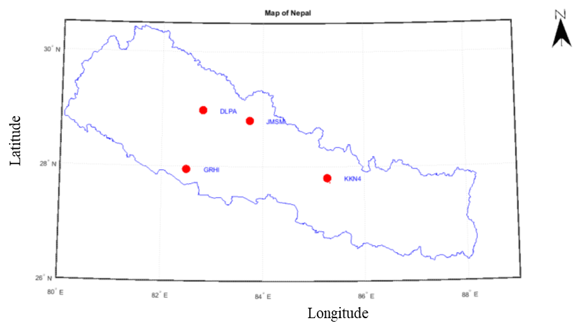
Figure 1A map of Nepal showing locations of GPS stations used in our study.
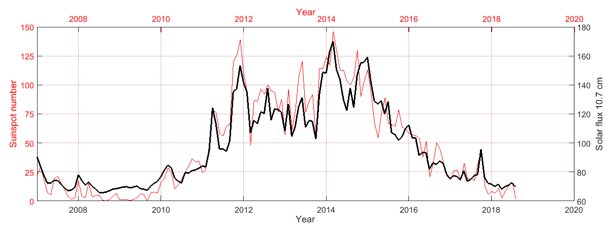
Figure 2Display the variations in the sunspot numbers and solar flux for the year 2008 to 2018.
3.1 Diurnal variation
Figure 3a exemplifies the diurnal variation in VTEC in LT observed during 2 February 2009, 2012, 2014, 2016 and 2017 during the minimum, inclining, maximum and declining phases of solar cycle 24 at the KKN4 station in Nepal. The plot shows that, before sunrise ∼05:00 LT, VTEC becomes minimum and reaches a maximum around 11:00–14:00 LT and later decreases in the evening and at night. The diurnal peak is noticed between 11:00 and 14:00 LT, though the peak values change every month. The VTEC plots reveal a growth from dawn to a highest value of about 5 to 98 TECU after the daylight hours, and it decreases to the lowest value prior to dusk, with a time difference of ±1 to 2 h. A flat curve with minor peaks is identified during the minimum and descending phases, whereas the dome shape is noticed during the maximum phase and multiple peaks and troughs at varying positions are observed during ascending phases. Overall, the VTEC shows a normal trend of diurnal behaviour, with the lowest values at dawn and dusk and the highest value during the midday. The maximum vertical total electron content values in the diurnal curve were noticed during the maximum phases of the solar cycle in 2014 and 2012 during the ascending phases, whereas the minimum values were observed in 2016, 2017 and 2009 during the descending phases. The diurnal variation in VTEC was studied by plotting similar curves for all the days from years 2008 to 2018 for all four chosen stations. In general, the diurnal VTEC behaviour exhibits a solar cycle dependency. The diurnal variability in VTEC for all the days is not presented due to constraint of space. In our study, the mean diurnal curves for the KKN4 station for years 2008, 2009 and 2010 exhibit a wave-like profile, whereas the mean diurnal curves of years 2011–2017 show a parabolic nature, which is shown in Fig. 3b. The similar diurnal profile was noticed for all stations considered. The diurnal graphs (Fig. 3) show a better synchronization of VTEC with SSN and solar flux (Fig. 2).
The observed diurnal VTEC pattern reflects the signature of different solar events. The noon bite-out profile with asymmetric peaks, parabolic profile and wave profile with morning, evening and night peaks and a few complex structures are noted in the diurnal profile. The quiet day activity at the minimum phase, the fluctuating activity during the increasing phase, shock activity during the maximum phase and recurrent activity during the declining phase was noticed in the study of ionospheric parameters at the Ouagadougou ionosonde station data in West Africa by Ouattara et al. (2009).
The upward E×B drift velocity plays an important role in producing the nighttime post-sunset enhancement. The average plasma flux required for the enhancement in equatorial latitude found by Jain (1987) in India. Tariku (2015) studied the pattern of GPS-TEC over the African sector during 2008 to 2009 and 2012 to 2013 and found small enhancements in the VTEC in the nighttime ∼ between 21:00 and 23:00 LT, especially for equinoctial months, and then drops again mostly after 23:00 LT. The enhancement was mostly found in equinoctial months during high solar activities, and during the low solar activities phase in the solstice, the pre-reversal enhancement was much smaller. A diurnal plot (Fig. 3) of the ionosphere over Nepal shows a similar result of pre-reversal enhancement during the high solar activities of 2012 and 2014 but not during the low solar activities of 2009 and 2017.
Mountains generate relief waves which propagate to the stratosphere and lower thermosphere (Leutbecher and Volkert, 2000). Studies on these waves have been made in Nepal in the lower atmosphere (Regmi and Maharjan, 2015; Regmi et al., 2017). Other studies have shown the impact of relief waves on the ionosphere in the Andes (Torre et al., 2014) and Tibet (Khan and Jin, 2018). In Fig. 3a, we see oscillations which cannot be interpreted directly as the signature of the waves. In fact, for the processing of GPS data, we use pseudo-range signals which can be affected by reflections on surrounding reliefs and by waves.
3.2 Monthly variation in TEC
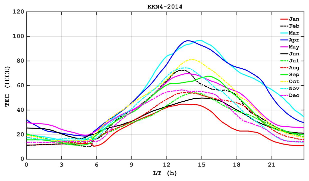
Figure 4 shows the monthly variability in VTEC for the maximum phase of solar cycle year 2014 at KKN4 station. The plot is obtained using the average of the daily data. The plot shows the maximum in equinoctial months (March and April) and the minimum in solstices (January and June). The rise or fall of TEC in each curve follows the diurnal pattern, which is the prominent peak in the midday with different peak amplitude. The lowest VTEC peak is observed during January and the highest in March. Late afternoon peak are seen in March, June and September, whereas the peak centred at ∼02:00 LT for rest of the months. A significant plat peak is noticed in December, whereas the steep rise in VTEC is noticed in March, April and October. The monthly variation in VTEC was studied by plotting similar curves for all the months from years 2008 to 2018 for all four chosen stations. The plot shows clear wave activity in the mean diurnal curve for years 2008, 2009 and 2010, and from the years 2011 to 2017 the stiff rise in VTEC was noticed (plots are not included in this paper). In general, the sunrise times in summer and winter are 05:15 and 06:45 LT, which differ by 1.5 h. During summer 2014, the maximum and minimum TEC observed is 21 and 12 TECU, whereas in winter the maximum and minimum TEC noticed is 25 and 15 TECU, respectively (Fig. 4). It also seems that during sunrise time in summer the VTEC is linear, but during the winter it is steep.
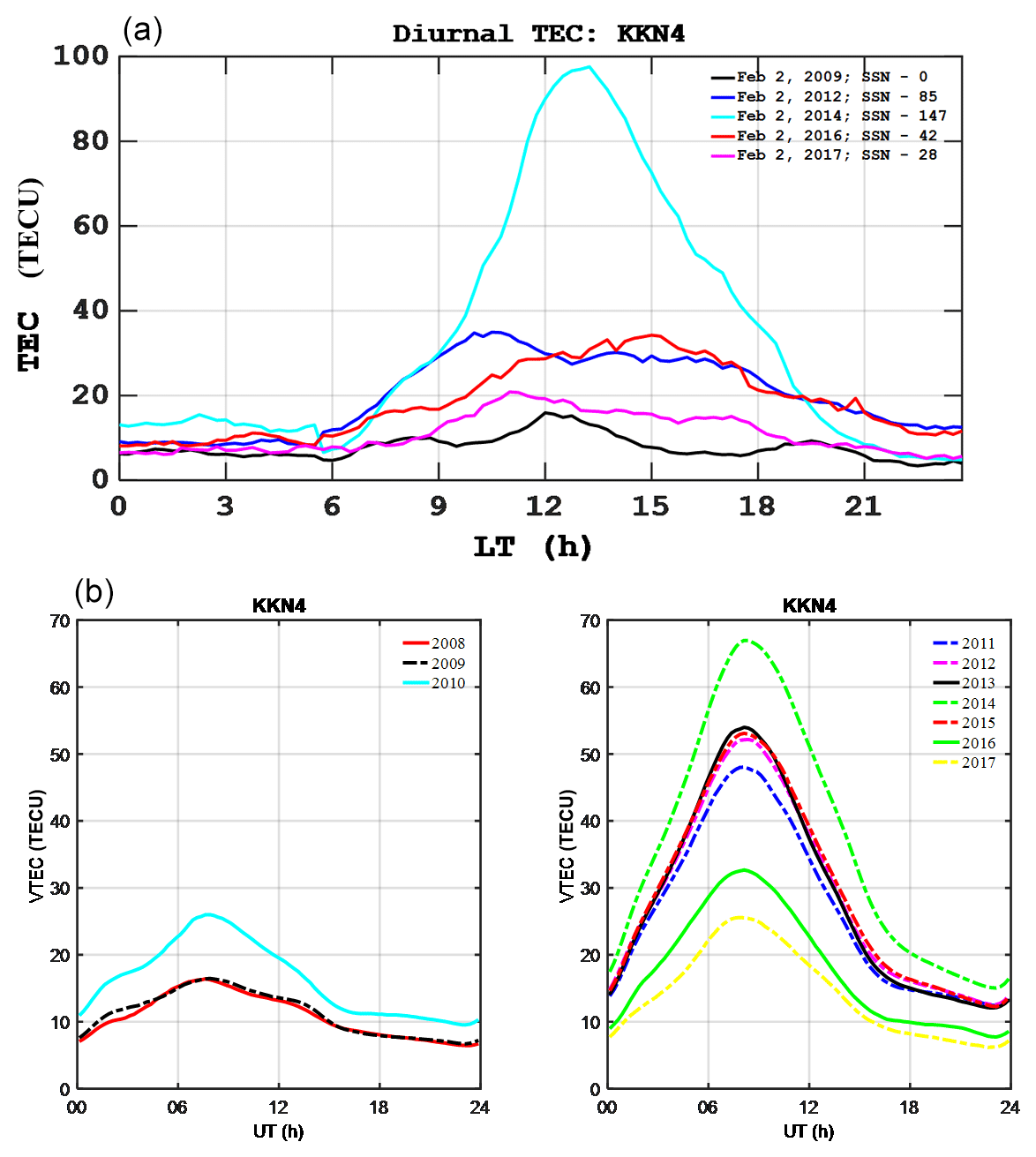
Figure 3(a) Diurnal variation in vertical TEC at KKN4 GPS station. The black, blue, light green, red and pink colour lines represent the diurnal variation for the years 2009, 2012, 2014, 2016 and 2017. (b) Yearly mean diurnal variation in vertical TEC; the left represents the wave-like nature and the right represents the parabolic nature.
3.3 Seasonal variation in TEC
Figure 5 shows a 2D diurnal plot of VTEC at JMSM station for all four phases (I minimum – 2009; II ascending – 2011; III maximum – 2014; IV descending – 2015) of solar cycle 24, which explains how the diurnal VTEC varies hourly during the four phases. In the ionosphere over Nepal, the features of equinoctial asymmetry is distinctly noticed in 2D plots of years 2009, 2011, 2014 and 2015 in Fig. 5a–d, respectively. From Fig. 5a–d, it can be observed that equinoctial asymmetry is not noticed in 2009, in 2011 autumn is more intense than spring, and in 2014 and 2015 spring VTEC is greater than autumn. In the year 2009, equinoctial asymmetry is not noticed during low solar activities. But in the year 2011, the autumn is more intense than spring, which is a feature of the equatorial ionization anomaly (EIA) crest latitude, and in the year 2014, the difference between equinoctial asymmetry is less (spring > autumn), which is again characteristic of the EIA trough station. And in 2015, the asymmetry very high (spring > autumn), which is the general feature of TEC at all latitudes.
In Fig. 6a–e, each panel separately represents the VTEC variation during the autumn, spring, summer and winter seasons for the years 2008, 2009, 2011, 2014 and 2015 at KKN4, GRHI, JMSM and DLPA, respectively. The plots show that the maximum value of VTEC is ∼95 TECU in spring 2014, which is the maximum year of the sunspot cycle, and the minimum value is 10 TECU in 2009 winter, which is the minimum year of the sunspot cycle. In the increasing and decreasing phases of solar cycle, the VTEC gradually increases and decreases, depending on the amount of UV that arrives at the Earth. In general, the plots show that VTEC is maximum during spring followed by autumn, summer and winter, except for a few cases. Similarly, previous studies of GPS TEC for the year 2014 over Nepal also reported the highest value of VTEC in March and lowest in December, with distinct the seasonal variations and having higher values in spring and lower in the winter season (Ghimire et al., 2020b). During the sunspot minimum years of 2008–2010, there are no semiannual variations in the VTEC, and it also seems that the summer VTEC is as strong as the autumn VTEC. For the years 2011 to 2016 the semiannual variations are noticed. During the year 2017, we observed the same pattern as for the years 2008–2010, where the summer VTEC is as strong as the autumn VTEC. At the station KKN4, the VTEC in autumn is very weak in year 2015, and it is smaller than the VTEC in summer. In year 2011, the VTEC is larger in winter than in summer at KKN4, whereas at GRHI and JMSM the winter VTEC is smaller than the summer one in years 2011 and 2014. At DLPA, the winter VTEC is not larger than the summer VTEC. In year 2008, the spring VTEC identified more than the autumn value for GRHI, JMSM and DLPA but less than the autumn value is observed at KKN4. In year 2009, only at JMSM, spring noticed greater values than autumn. The autumn VTEC is greater than spring for all stations in 2011, except at JMSM where it is equal to spring. Large asymmetry is noticed between spring and autumn in year 2014. In year 2015, the summer peak is higher than the autumn. In the present study the VTEC is larger in winter than the VTEC in summer that is noticed in 2011 and 2014. At KKN4 station, a VTEC that is larger in winter than the VTEC in summer is noticed in the year 2014, and the same applies at GRHI in 2014 and 2016 and at JMSM 2014 and 2016. The VTEC that is larger in winter than in summer is not noticed at DLPA (Fig. 6c and d).
The solar flux dependency of the winter anomaly in GPS TEC has been studied by Rao et al. (2019b). The result showed that, when the level of solar flux in winter month is greater than the corresponding summer month, the winter anomaly is observed irrespective of whether the phases of solar cycle are is high or low. Their study also pointed out that the winter anomaly in GPS-derived TEC may not be a feature of any geophysical significance. The winter or seasonal anomaly is introduced due to temperature changes (Appleton, 1935), interhemispheric transport of ionization (Rothwell, 1963), significant changes in the Sun–Earth distance (Yonezawa, 1959; Buonsanto, 1986), seasonal variation in concentration (Rishbeth and Setty, 1961; Wright, 1963; Rishbeth et al., 2000; Zhang et al., 2005) and the upward movement of energy flux (Maeda et al., 1986). The winter anomaly is related to solar activity. Tyagi and Das Gupta (1990) and Bagiya et al. (2009) have reported an absence of the winter anomaly in low solar activities at low latitudes. The change in composition of the constituents being identified as the cause of the winter anomaly was coined by Rishbeth and Setty (1961). The least VTEC in the June solstice (in the Northern Hemisphere) during the low and high solar activity phase may be due to the asymmetric heating, which results in the transport of neutral constituents from the summer to the winter hemisphere, reducing the rate of recombination. The reduction in the recombination rate in winter causes the greater rise of VTEC in winter than in summer. Gupta and Singh (2000) studied TEC over Delhi and concluded that the winter anomaly in TEC appears only during higher solar activity. This winter anomaly is due to the closer distance of the Earth to the Sun and the direction of the wind from the summer season to the winter (Shimeis et al. 2014). Krankowsky et al. (1968) and Cox and Evans (1970) separately pointed out that the ratio of becomes twice its value in winter than in summer as a result of higher electron loss rate in summer than in winter. Torr and Torr (1973) observed the winter anomaly in the critical frequency of ionospheric F2 layer (foF2) under different solar activity at the mid latitude of the Northern Hemisphere, and a similar result was observed in the Southern Hemisphere during high solar activity. Furthermore, they noticed that lower solar activity results equal a lower winter anomaly. In general, the June solstice anomaly is higher than the December solstice, but in an earlier study done at Agra GPS station, they noticed some abnormalities in the solstice behaviour, demonstrating higher VTEC in the summer anomaly than the autumn and winter anomalies, with higher VTEC than in summer (Bagiya et al., 2011).
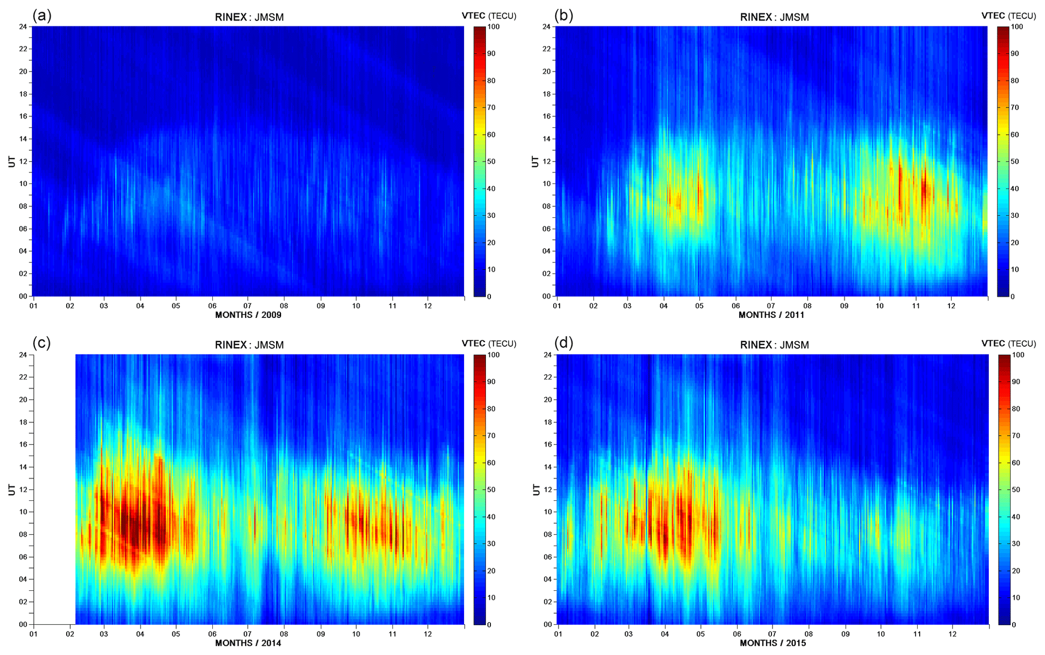
Figure 5(a–d) A two-dimensional (2D) variation in vertical TEC according to UT at the JMSM station for one of the years of the minimum (2009), ascending (2011), maximum (2014) and descending (2015) phases of solar cycle 24.
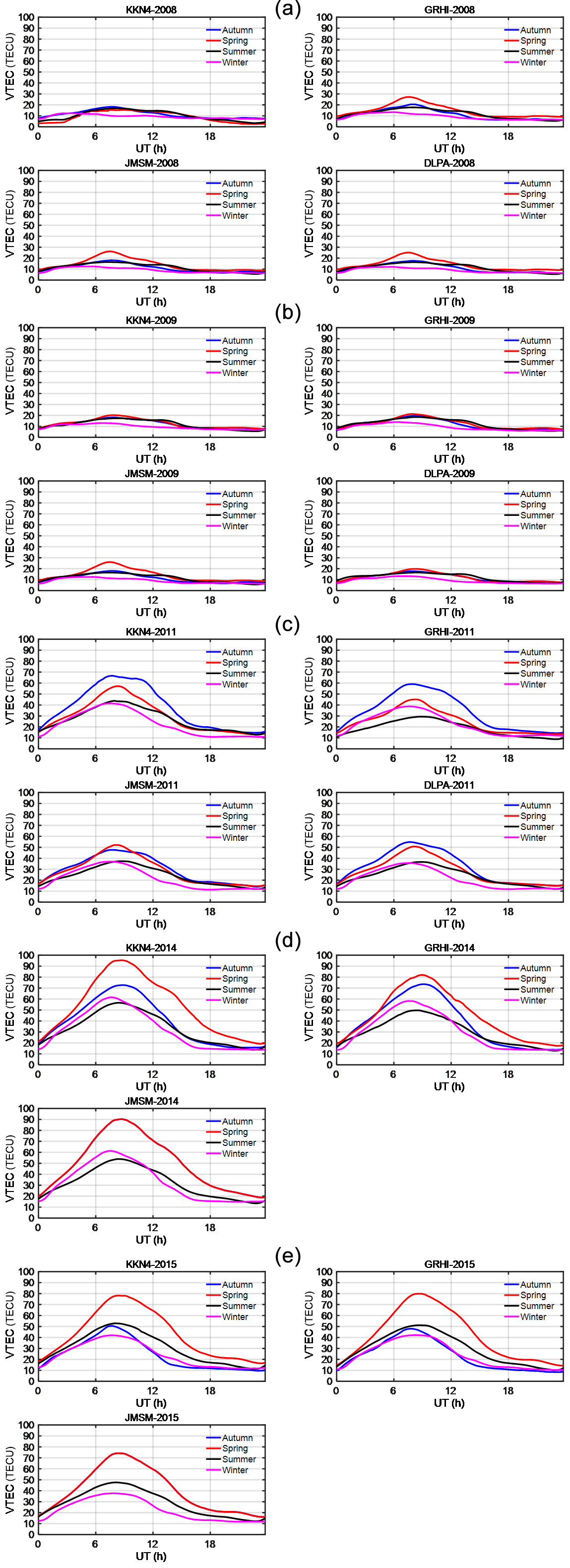
Figure 6Seasonal variability in VTEC during years 2008 (a), 2009 (b), 2011 (c), 2014 (d) and 2015 (e) for KKN4, GRHI, JMSM and DLPA stations.
In Fig. 7, the top left panel represents the variation in VTEC during spring, bottom left during autumn, top right during summer and bottom right during winter from 2008 to 2017 at KKN4. In spring, the difference in VTEC between high and low solar activity is 65 TECU, in autumn it is 53 TECU, in summer it is 45 TECU, and in winter it is 40 TECU, respectively. In Fig. 8, the top panel represents VTEC variability during the minimum and increasing phases, whereas the bottom panel represents the maximum and decreasing phases of solar cycle 24 using the GPS station at GRHI. The plot shows that equinoctial asymmetry is not observable during the minimum solar of cycle 2008 and 2009, but it is clearly distinguishable during other phases of solar cycle.

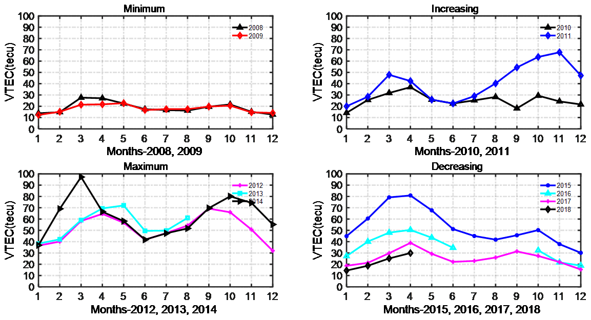
Figure 8VTEC variability in GRHI station during minimum, increasing, maximum and decreasing phases of solar cycle 24.
The important parameter for the semiannual variation in ionospheric ionization is the variation in the atomicmolecular ratio, i.e. the concentration of the ratio. At the solstice, there is circulation of the meridional wind of about 25 m s−1 in the middle and low latitudes from summer to winter hemisphere (Rishbeth et al., 2000). These winds carry nitrogen-rich air produced in the summer hemisphere into lower latitudes by upwelling in higher latitudes, thus reducing ratio. At the equinox, there is no prevailing meridional circulation. The ratio depends specially on the horizontal circulation, and its seasonal changes accompany the change in global thermospheric circulation between the pattern from summer to winter around the solstices to a symmetrical pattern at equinoxes. The six possible reasons for seasonal and semiannual variations in the F2 layer, discussed by Rishbeth (1998), are as follows: (a) the compositional changes due to large-scale dynamical effects in the thermosphere, (b) variations in the geomagnetic activities, (c) energy of the solar wind, (d) the inputs from lower atmospheric phenomena such as waves and tides, (e) change in atmospheric turbulence and (f) anisotropy of solar and EUV emissions in the solar latitude (Burkard, 1951).
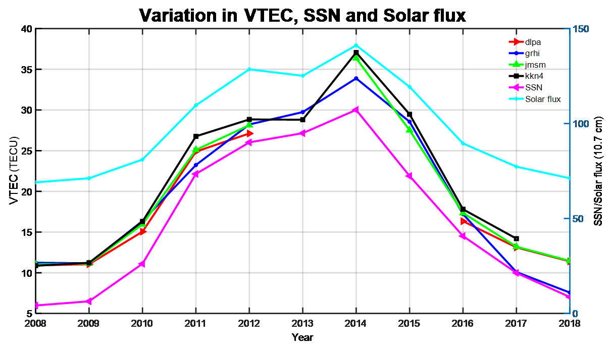
Figure 9Annual mean VTEC variability in the KKN4, GRHI, JMSM and DLPA stations for the SSN and solar flux during year 2008–2018.
In 2019, Ansari et al. (2019) found the minimum value of TEC in January, which becomes a maximum in April, decreases in June–July and is followed by an increase in magnitude of the second maximum in September–October and later a decrease until December at CHLM, JMSM and GRHI in year 2017. Referring to Fig. 8, our result for semiannual variation shows that the minimum value of VTEC is found in January, which becomes the maximum in March–April, decreases in June–July, is followed by an increase in magnitude of the second maximum in October–November and later decreases until December at GRHI in years 2009 to 2018.
The asymmetry between the two equinoxes is due to geophysical parameters as magnetic indices related to geomagnetic activity (Triskova, 1989) and the interplanetary magnetic field (IMF Bz) the interplanetary component of magnetic field (Russell and McPherron, 1973). The equinoctial asymmetry observed in VTEC is explained by (i) the axial hypothesis (ii) the Russell–McPherron (RM) effect and (iii) the equinoctial hypothesis (Lal, 1996; Shimeis et al., 2014).
Ouattara and Amory-Mazaudier (2012) made a statistical model of the F2 layer, at equatorial latitudes, based on data obtained during three sunspot cycles. This model shows the influence of the different types of geomagnetic activity defined by Legrand and Simon (1989) and the asymmetry of equinoxes due to the magnetic activity. The asymmetry between the two equinoctial peaks is also due to the asymmetry of the thermospheric parameters that influence the ionosphere as neutral wind and changes in composition (Balan et al., 1998)
3.4 Solar cycle variation in TEC
Figure 9 shows the annual mean values of VTEC, solar flux index and sunspot number during the solar cycle from years 2008 to 2018. The black, blue, green and red lines represent the VTEC variation at stations KKN4, GRHI, JMSM and DLPA, whereas pink and light green lines represents variation in SSN and solar flux index, respectively. The plot shows that VTEC gradually begins to increase in 2009 and reaches a maximum in 2014. Then it begins to decrease until 2018, which agrees with the sunspot number and solar flux variation in the same plot. The figure shows that the maximum value of the peak of ionization in 2014 is about 37 TECU in the maximum phase of the solar cycle, and the minimum value in 2008 is about 11 TECU in the minimum phase of solar cycle. The observed VTEC variation corresponds to the amount of UV reaching the Earth.
Similarly, the solar flux increases are from 2011 onward; the measured VTEC also exhibits the highest magnitude for the year 2014. The maximum VTEC value shows a decreasing trend from years 2015 to 2018 at all the stations used for this study. It is observed from the graph that the average annual VTEC shows better synchronization with SSN and solar flux index.
The patterns of the solar cycles play a major role in the solar variability, i.e. solar radiation and sunspot number consequently influence the ionosphere. Solar cycle 24 is the smallest solar cycle since the start of the spatial era (1957), in which a peak is noticed in 2014 and a few major solar flares erupted from the Sun in February and October 2014 (Kane, 2002), so the maximum VTEC is noticed in February and October as shown in Fig. 8. Again, from Fig. 8, a higher value for sunspot and solar flux was reported in February 2011, corresponding to an X-class solar flare at which a higher value of VTEC was noted in station considered. Sharma et al. (2012) studied how the VTEC variation in Delhi lies near the equatorial crest region during low solar activities in years 2007 to 2009 and found that TEC has a short-lived day minimum between 05:00–06:00 LT and gradual increase, and it reaches its peak value between 12:00 and 14:00 LT. The day minimum was found to be flat during most of the nighttime hours (22:00 to 06:00 LT). Their results show a magnitude of daily maximum TEC decreases from 2007 to 2009 due to decreases in the solar flux. They also found TEC seasonal behaviour depends on the solar cycle, and the largest daily TEC is observed during the equinoctial month at Delhi. In 2020, Ghimire et al. (2020a), studied the diurnal variation in TEC at JMJG (Lamjung, Nepal) station for the year 2015 and found the minimum in the pre-dawn, a steady increase in the early morning followed by afternoon maximum and then a gradual decrease after sunset; a similar pattern is also observed our study.
In the African sector, Tariku (2015) observed, from 2008 to 2009 and 2012 to 2013, high values of VTEC during the low and high solar activity phases. According to their findings, the diurnal VTEC values attained a maximum in the time interval of 13:00 to 16:00 LT, and the least values are mostly at around 06:00 LT. A similar result is noticed in all considered Nepalese GPS stations during the low solar active phases of solar cycle 24 in Nepal. The maximum diurnal variability in the VTEC in 2014 is caused by a solar active period confirmed by maximum sunspot number (SSN) and solar flux index (shown in Fig. 2). The VTEC is greater in 2012 due to the second maximum in SSN and solar flux, and the minimum VTEC in 2009 and 2017 is supported by the minimum SSN and solar flux, which is confirmed by the synchronization of VTEC with SSN and solar flux (Fig. 9). In the ionosphere over Nepal, the diurnal VTEC maximum occurs approximately between 12:00 to 14:00 LT. Similar to Delhi station in Nepal, the day minimum was found to be flat during most of the nighttime hours (22:00 to 06:00 LT). In general, the value of diurnal peak in VTEC is maximum during the spring equinoxes, except in 2011 in which the autumn VTEC is maximum. As the solar flux decreases from 2008 to 2009, the daily maximum VTEC values show a decreasing trend.
This paper investigates the diurnal, monthly, seasonal and solar cycle variations in VTEC at four mid–low latitude stations, namely KKN4 (27.80∘ N, 85.27∘ E), GRHI (27.95∘ N, 82.49∘ E), JMSM (28.80∘ N, 83.74∘ E) and DLPA (28.98∘ N, 82.81∘ E) in Nepal.
The following conclusions are found:
-
The shape of the mean diurnal variation in VTEC depends on the solar cycle phases, i.e. a flat diurnal peak is observed during minimum and descending phases of the solar cycle, whereas a Gaussian with different peak amplitude is noticed during the ascending and maximum phases of the solar cycle.
-
The study may reveal that diurnal TEC maximizes at around 11:00 to 14:00 LT, with a minimum in the pre-dawn periods.
-
Day-to-day variation in VTEC is significant in all the station. The maximum is noticed at KKN4 and the minimum at DLPA.
-
The mean diurnal profile in the years 2008, 2009 and 2010 exhibit a wave-like nature, whereas a parabolic nature is observed in the years 2011, 2012, 2013, 2014, 2015, 2016 and 2017.
-
The week ionospheric activities are characterized by lower TEC values during the minimum phase, and strong activities are characterized by a higher value of VTEC during the maximum phase, i.e. VTEC has shown proper synchronization with SSN and solar flux.
-
The monthly plot shows that, during the sunrise time in summer, the VTEC is linear, whereas it is steep during the winter.
-
Equinoctial asymmetry is not noticed in 2009; in 2011, the autumn is more intense than the spring, and in 2014 and 2015, the spring VTEC is greater than the autumn.
-
Equinoctial asymmetry peaks are noticed in spring (March and April) and autumn (September and October), with higher values being observed during spring.
-
The equinoctial asymmetry is noticed in all the available stations due to difference in the F10.7 cm for the two equinoxes.
-
The spring maximum is smaller than autumn maximum, mainly during years 2011–2013 and also during year 2008 for one station; these years are years of the minimum or increasing phase of the sunspot cycle.
-
The VTEC in winter is greater than the VTEC in summer and is observed in all the available stations at the maximum of the sunspot cycle in 2014 and in one other station during the year 2011.
-
During the year 2009 of the sunspot minimum, the VTEC in winter is greater than the VTEC in summer and is not observed for all the stations. There is no equinoctial asymmetry, i.e. it is very weak (compare to the year of the maximum), except at JMSM.
-
It seems that, in Nepal for some years, there is no semiannual variation, as we observe sometimes that the summer VTEC is larger than VTEC in the autumn.
The highest Himalayan mountains on Earth in Nepal are the source of landform waves that travel through the stratosphere and the lower thermosphere, where they deposit their energy and give birth to secondary gravity waves that can affect VTEC. In our climatology study, we analyse average behaviours that do not allow the study of these waves. Another study analysing each day individually and using the phase processing of GPS signals should be done in the future to analyse the impact of the Himalayas on VTEC and the impact of the low atmosphere on VTEC.
The data for this study are available at http://www.unavco.org (last access: 15 March 2020), http://aiuws.unibe.ch/ionosphere (last access: 15 March 2020) (CODG), http://www.ngs.noaa.gov/CORS/Gpscal.shtml (last access: 15 March 2020), http://www.isgi.unistra.fr/ (last access: 15 March 2020), http://celestrack.com/GPS/almanar/Yuma/2017/ (last access: 15 March 2020), http://sidc.oma.be/silso/home (last access: 6 April 2020) and the OmniData site http://omniweb.gsfc.nasa.gov/ (last access: 6 April 2020) for GPS TEC data in RINEX, DCB and Yuma files. The sunspot number and solar flux and data for solar wind parameters and geomagnetic indices, respectively, are used.
DP developed the idea of this paper, prepared introduction, collected the data sets and contributed to the methodology and conclusions. BG contributed in writing the discussion of the results. CAM contributed to the data set and data analysis and conclusion, assisted with editing the paper and helped shape the paper. RF provided the software for this study and contributed to the methodology and editing of the text. NPC gave overall feedback on this paper by reviewing the paper thoroughly and giving the complete paper a shape. BA contributed to the results and discussion and reviewed the paper thoroughly.
The authors declare that they have no conflict of interest.
Publisher's note: Copernicus Publications remains neutral with regard to jurisdictional claims in published maps and institutional affiliations.
We acknowledge http://www.unavco.org, https://www.aiub.unibe.ch/download/CODE (CODG), http://www.ngs.noaa.gov/CORS/Gpscal.shtml and https://isgi.unistra.fr, as well as http://celestrack.com/GPS/almanar/Yuma/2017/ http://sidc.oma.be/silso/home and the OmniData site http://omniweb.gsfc.nasa.gov/ for providing RINEX data for TEC, DCB and Yuma files and data for solar wind parameters and geomagnetic indices for our calculations. Drabindra Pandit would like to acknowledge the Nepal Academy of Science and Technology (NAST), Nepal, for proving doctoral scholarship and ICTP, Italy, for giving the opportunity to participate in a workshop on space weather effects on Global Navigation Satellite System (GNSS) operations at low latitudes.
This paper was edited by Dalia Buresova and reviewed by S.S. Rao and two anonymous referees.
Akala, A. O., Rabiu, A. B., Somoye, E. O., Oyeyemi, E. O., and Adeloye, A. B.: The Response of African equatorial GPS TEC to intense geomagnetic storms during the ascending phase of solar cycle 24, J. Atmos. Sol. Terr.-Phy., 98, 50–62, https://doi.org/10.1016/j.jastp.2013.02.006, 2013.
Ansari, K., Park, K. D., and Panda, S. K.: Empirical and orthogonal function analysis and modeling of ionospheric TEC over South Korean region, Acta Astronaut., 161, 313–324, https://doi.org/10.1016/j.actaastro.2019.05.044, 2019.
Anderson, D. and Fuller-Rowell, T.: The ionosphere, Space environment topics SE-14, Report, Space Environment Center, Boulder, 1999.
Appleton, E. V. and Ingram, L. J.: Magnetic Storms and Upper-Atmospheric Ionisation, Nature, 136, 548–549, https://doi.org/10.1038/136548b0, 1935.
Bagiya, M. S., Joshi, H. P., Iyer, K. N., Aggarwal, M., Ravindran, S., and Pathan, B. M.: TEC variations during low solar activity period (2005–2007) near the Equatorial Ionospheric Anomaly Crest region in India, Ann. Geophys., 27, 1047–1057, https://doi.org/10.5194/angeo-27-1047-2009, 2009.
Bagiya, M. S., Iyer, K. N., Joshi, H. P., Tsugawa, T., Ravindra, S., Sridharan, R., and Pathan, B. M.: Low-latitude ionospheric-thermospheric response to storm time electro dynamical coupling between high and low latitudes, J. Geophys. Res., 116, A01303, https://doi.org/10.1029/2010JA015845, 2011.
Balan, N., Batista, I. S., Abdu, M. A., Macdougall, J., and Bailey, G. J.: Physical mechanism and statistics of occurrence of an additional layer in the equatorial ionosphere, J. Geophys. Res., 103, 169–181, https://doi.org/10.1029/98JA02823, 1998.
Buonsanto, M. J.: Possible effects of the changing Earth-Sun distance on the upper atmosphere, S. Pacific J. Nat. Sci, 8, 58–65, available at: https://uspaquatic.library.usp.ac.fj/gsdl/collect/spjnas/index/assoc/HASHd462.dir/doc.pdf (last access: 23 June 2021), 1986.
Burkard, O.: Die halbjährige Periode der F2-Schicht-Ionisation, Arch. Meteor. Geophy. A, 4, 391–402, https://doi.org/10.1007/BF02246815, 1951.
Chauhan, V., Singh, O. P., and Singh, B.: Diurnal and seasonal variation of GPS-TEC during a low solar activity period as observed at a low latitude station Agra, Indian J. Radio Space, 40, 26–36, available at: http://nopr.niscair.res.in/handle/123456789/11195 (last access: 23 June 2021), 2011.
Cox, L. P. and Evans, J. V.: Seasonal variation of the ratio in the F1 region, J. Geophy. Res., 75, 6271, https://doi.org/10.1029/JA075i031p06271, 1970.
D'ujanga, F. M., Mubiru, J., Twinamasiko, B. F., Basalirwa, C., and Ssenyonga, T. J.: Total Electron Content Variations in Equatorial Anomaly Region, Adv. Space Res., 50, 441–449, https://doi.org/10.1016/j.asr.2012.05.005, 2012.
Dabas, R. S., Lakshmi, D. R., and Reddy, B. M.: Solar activity dependence of ionospheric electron content and slab thickness using different solar indices, Pure Appl. Geophys., 140, 721–728, https://doi.org/10.1007/BF00876585, 1993.
Dashora, N. and Suresh, S. : Characteristics of low-latitude TEC during solar cycles 23 and 24 using global ionospheric maps (GIMs) over Indian sector, J. Geophys. Res.-Space, 120, 5176–5193, https://doi.org/10.1002/2014JA020559, 2015.
de Abreu, A. J., Fagundes, P. R., Gende, M., Bolaji, O. S., de Jesus, R., and Brunini, C. : Investigation of ionospheric response to two moderate geomagnetic storms using GPS-TEC measurements in the South American and African sectors during the ascending phase of solar cycle 24, Adv. Space Res., 53, 1313–1328, https://doi.org/10.1016/j.asr.2014.02.011, 2014.
Galav, P., Dashora, N., Sharma, S., and Pandey, R.: Characterization of low latitude GPS-TEC during very low solar activity phase, J. Atmos. Sol. Terr.-Phy., 72, 1309–1317, https://doi.org/10.1016/j.jastp.2010.09.017, 2010.
Ghimire, B. D., Chapagain, N. P., Basnet, V., Bhatt, K., and Khadka, B.: Variation of Total Electron Content (TEC) in the quiet and disturbed days and their correlation with geomagnetic parameters of Lamjung Station in the year of 2015, Bibechana, 17, 123–132, available at: https://www.nepjol.info/index.php/BIBECHANA/article/view/26249/22107 (last access: 17 March 2021), 2020a.
Ghimire, B. D., Chapagain, N. P., Basnet, V., Bhatta, K., and Khadka, B.: Variation of GPS- TEC Measurements of the Year 2014: A Comparative Study with IRI – 2016 Model, Journal of Nepal Physical Society, 6, 90–96, https://doi.org/10.3126/jnphyssoc.v6i1.30555, 2020b.
Guo, J., Li, W., Liu, X., Kong, Q., Zhao, C., and Guo, B.: Temporal-spatial variation of global GPS-derived total electron content, 1999–2013, PloS ONE, 10, e0133378, https://doi.org/10.1371/journal.pone.0133378, 2015.
Gupta, J. K. and Singh, L.: Long term ionospheric electron content variations over Delhi, Ann. Geophys., 18, 1635–1644, https://doi.org/10.1007/s00585-001-1635-8, 2000.
Hofmann-Wellenhof, B., Lichtenegger, H., and Collins, J.: GPS: Theory and Practice, Springer Verlag, Wien, ISBN 978-3-211-82364-6 and 978-3-7091-3298-5 (eBook), 1992.
Huo, X. L., Yuan, Y. B., Ou, J. K., Zhang, K. F., and Bailey, G. J.: Monitoring the Global-Scale Winter Anomaly of Total Electron Contents Using GPS Data, Earth Planets Space, 61, 1019–1024, https://doi.org/10.1186/BF03352952, 2009.
Jain, A. R.: Reversal of E×B drift & post sunset enhancement of the ionospheric total electron content at equatorial latitudes, Indian J. Radio Space, 16, 267–272, available at: http://nopr.niscair.res.in/handle/123456789/36497 (last access: 26 June 2021), 1987.
Kane, R. P.: Some implications using the group sunspot number reconstruction, Sol. Phys., 205, 383–401, https://doi.org/10.1023/A:1014296529097, 2002.
Khan, A. and Jin, S.: Gravity wave activities in Tibet observed by Cosmic GPS radio occultation, Geodesy and Geodynamics., 9, 504–511, https://doi.org/10.1016/j.geog.2018.09.009, 2018.
Kramkowsky, D., Kasprazak, W. T., and Nier, A. O.: Mass spectrometric studies of the composition of the lower thermosphere during summer 1967, J. Geophys. Res., 73, 7291–7306, https://doi.org/10.1029/JA073i023p07291, 1968.
Lal, C.: Seasonal trend of geomagnetic activity derived from solar-terrestrial geometry confirms an axial-equinoctial theory and reveals deficiency in planetary indices, J. Atmos. Terr. Phys., 58, 1497–1506, https://doi.org/10.1016/0021-9169(95)00182-4, 1996.
Legrand, J. P. and Simon, P. A.: Solar cycle and geomagnetic activity: A review for geophysicists. Part I. The contributions to geomagnetic activity of shock waves and of the solar wind, Ann. Geophys., 7, 565–578, available at: http://www.ipgp.jussieu.fr/~legoff/Download-PDF/Soleil-Climat/IndicesAA/annales-geophysicaeI-89-7-565-578.pdf (last access: 23 June 2021), 1989.
Martin, L. and Volkert, H.: The Propagation of Mountain Waves into the Stratosphere: Quantitative Evaluation of Three-Dimensional Simulations, J. Atmos. Sci., 57, 3090–3108, https://doi.org/10.1175/1520-0469(2000)057<3090:TPOMWI>2.0.CO;2, 2000.
Liu, L. B., Wan, W. X., Ning, B. Q., and Zhang, M. L.: Climatology of the mean total electron content derived from GPS global ionospheric maps, J. Geophys. Res., 114, A06308, https://doi.org/10.1029/2009JA014244, 2009.
Liu, G., Huang, W., Gong, J., and Shem, H.: Seasonal variability of GPS-VTEC and model during low solar activity period 2006–2007 near the equatorial ionization anomaly crest location in Chinese zone, Adv. Space Res., 51, 366–376, https://doi.org/10.1016/j.asr.2012.09.002, 2013.
Liu, L. B. and Chen, Y. D. : Statistical analysis of solar activity variations of total electron content derived at Jet Propulsion Laboratory from GPS observations, J. Geophys. Res., 114, A10311, https://doi.org/10.1029/2009JA014533, 2009.
Maeda, K., Hedin, A. E., and Mayr, H. G.: Hemispheric asymmetries of the thermospheric semiannual oscillation, J. Geophys. Res.-Space, 91, 4461–4470, https://doi.org/10.1029/JA091iA04p04461, 1986.
Mansoori, A. A., Parvaiz, A. K., Rafi, A., Roshni, A., Aslam, A. M., Shivangi, B., Bhupendra, M., Purohit, P. K., and Gwal, A. K.: Evaluation of long term solar activity effects on GPS derived TEC, J. Phys. Conf. Ser., 759, 012069, https://doi.org/10.1088/1742-6596/759/1/012069, 2016.
Natali, M. P. and Meza, A.: Annual and semiannual variations of vertical total electron content during high solar activity based on GPS observations, Ann. Geophys., 29, 865–873, https://doi.org/10.5194/angeo-29-865-2011, 2011.
Parwani, M., Atulkar, R., Mukherjee, S., and Purohit, P. K.: Latitudinal variation of ionospheric TEC at northern hemispheric region, Russian Journal of Earth Sciences, 19, ES1003, https://doi.org/10.2205/2018ES000644, 2019.
Perevalova, N. P., Polyakova, A. S., and Zalizovski, A. V.: Diurnal Variation of the Total Electron Content under Quiet Helio-Geomagnetic Conditions, J. Atmos. Sol. Terr.-Phy., 72, 997–1007, https://doi.org/10.1016/j.jastp.2010.05.014, 2010.
Prikryl, P., Jayachandran, P. T., Mushini, S. C., Pokhotelov, D., MacDougall, J. W., Donovan, E., Spanswick, E., and St.-Maurice, J.-P.: GPS TEC, scintillation and cycle slips observed at high latitudes during solar minimum, Ann. Geophys., 28, 1307–1316, https://doi.org/10.5194/angeo-28-1307-2010, 2010.
Ouattara, F. and Amory-Mazaudier, C.: Statistical study of the equatorial F2 layer at Ouagadougou during solar cycles 20, 21, 22 using Legrand and Simon's classification of geomagnetic activity, J. Space Weather Spac., 2, A19, https://doi.org/10.1051/swsc/2012019, 2012.
Ouattara, F. and Fleury, R.: Variability of CODG TEC and IRI 2001 Total Electron Content (TEC) during IHY Campaign Period (21 March to 16 April 2008) at Niamey under Different Geomagnetic Activity Conditions, Sci. Res. Essays, 6, 3609–3622, https://doi.org/10.5897/SRE10.1050, 2011.
Ouattara, F., Amory-Mazaudier, C., Fleury, R., Lassudrie Duchesne, P., Vila, P., and Petitdidier, M.: West African equatorial ionospheric parameters climatology based on Ouagadougou ionosonde station data from June 1966 to February 1998, Ann. Geophys., 27, 2503–2514, https://doi.org/10.5194/angeo-27-2503-2009, 2009.
Rama Rao, P. V. S., Nru, D., and Srirama Rao, M.: Study of some low latitude ionospheric phenomena observed in TEC measurements at Waltair, India, in: Proceedings COSPAR/URSI Symp. Warsaw, Poland, edited by: Wernik, A. W., 51, 19–23 May 1980.
Rao, S. S., Chakraborty, M., Kumar, S., and Singh, A. K.: Low-latitude ionospheric response from GPS, IRI and TIE-GCM TEC to Solar Cycle 24, Astrophys. Space Sci., 364, 216, https://doi.org/10.1007/s10509-019-3701-2, 2019a.
Rao, S. S., Sharma, S., and Pandey, R.: Study of solar flux dependency of the winter anomaly in GPS TEC, GPS Solut., 23, 4, https://doi.org/10.1007/s10291-018-0795-x, 2019b.
Regmi, R. P. and Maharjan, S.: Trapped mountain wave excitations over the Kathmandu valley, Nepal, Asia-Pac. J. Atmos. Sci., 51, 303–309, https://doi.org/10.1007/s13143-015-0078-1, 2015.
Regmi, R. P., Kitada, T., Dudha, J., and Maharjan, S.: Large-scale gravity over the middle hills of the Nepal Himalayas: implication for aircraft accidents, J. Appl. Meteorol. Clim., 56, 371–389, https://doi.org/10.1175/JAMC-D-16-0073.1, 2017.
Rishbeth, H.: How the thermospheric circulation affects the ionospheric F2-layer, J. Atmos. Sol.-Terr. Phy., 60, 1385–1402, https://doi.org/10.1016/S1364-6826(98)00062-5, 1998.
Rishbeth, H. and Setty, C. S. G. K.: The F-layer at sunrise, J. Atmos. Terr. Phys., 20, 263–276, https://doi.org/10.1016/0021-9169(61)90205-7, 1961.
Rishbeth, H., Müller-Wodarg, I. C. F., Zou, L., Fuller-Rowell, T. J., Millward, G. H., Moffett, R. J., Idenden, D. W., and Aylward, A. D.: Annual and semiannual variations in the ionospheric F2-layer: II. Physical discussion, Ann. Geophys., 18, 945–956, https://doi.org/10.1007/s00585-000-0945-6, 2000.
Rothwell, P.: Diffusion of ions between F layers at magnetic conjugate points, in Proceedings International Conference on the Ionosphere, Institute of Physics and Physical Society, London, 217–221, 1963.
Russell, C. T. and McPherron, R. L.: Semiannual variation of geomagnetic activity, J. Geophys. Res., 78, 92–108, https://doi.org/10.1029/JA078i001p00092, 1973.
Sahai, Y., Becker-Guedes, F., and Fagundes, P. R.: Response of Nighttime Equatorial and Low Latitude F-Region to the Geomagnetic Storm of August 18, 2003, in the Brazilian Sector, Adv. Space Res., 39, 1325–1334, https://doi.org/10.1016/j.asr.2007.02.064, 2007.
Sharma, K., Dabas, R. S., and Ravindran, S.: Study of total electron content over equatorial and low latitude ionosphere during extreme solar minimum, Astrophys. Space Sci., 341, 277–286, https://doi.org/10.1007/s10509-012-1133-3, 2012.
Shimeis, A., Amory-Mazaudier, C., Fleury, R., Mahrous, A. M., and Hassan, A. F.: Transient variations of vertical total electron content over some African stations from 2002 to 2012, Adv. Space Res., 54, 2159–2171, https://doi.org/10.1016/j.asr.2014.07.038, 2014.
Tariku, Y. A.: Patterns of GPS-TEC variation over low-latitude regions (African sector) during the deep solar minimum (2008 to 2009) and solar maximum (2012 to 2013) phases, Earth Planets Space, 67, 35, https://doi.org/10.1186/s40623-015-0206-2, 2015.
Titheridge, J. F.: The total electron content of the southern midlatitude ionosphere, 1965–1971, J. Atmos. Terr. Phys., 35, 981–1001, https://doi.org/10.1016/0021-9169(73)90077-9, 1972.
Torr, M. R. and Torr, D. G.: The seasonal behavior of the F2-layer of the ionosphere, J. Atmos. Terr. Phys., 35, 22–37, https://doi.org/10.1016/0021-9169(73)90140-2, 1973.
Torre, A., Alexander, P., Llamedo, P., Hierro, R., Nava, B., Radicella, S., Schmidt, T., and Wickert, J.: Wave activity at ionospheric heights above the Andes Mountains detected from FORMOSAT3/COSMIC GPS radio occultation data, J. Geophys. Res.-Space, 119, 2046–2051, 2014.
Triskova, L.: The vernal-autumn asymmetry in the seasonal variation of geomagnetic activity, J. Atmos. Terr. Phys., 51, 111–118, https://doi.org/10.1016/0021-9169(89)90110-4,1989.
Tyagi, T. R. and Das Gupta, A.: Beacon satellite studies and modeling of total electron content of ionosphere, Indian J. Radio Space, 424–438, available at: http://nopr.niscair.res.in/handle/123456789/36307 (last access: 23 June 2021), 1990.
Venkatesh, K., Fagundes, P. R., de Jesus, R., de Abreu, A. J., and Sumod, S. G.: Assessment of IRI-2012 Profile Parameters by Comparison with the Ones Inferred Using NeQuick2, Ionosonde and FORMOSAT-1 Data during the High Solar Activity over Brazilian Equatorial and Low Latitude Sector, J. Atmos. Sol. Terr.-Phy., 121, 10–23, https://doi.org/10.1016/j.jastp.2014.09.014, 2014a.
Venkatesh, K., Fagundes, P. R., Seemala, G. K., de Jesus, R., and Pillat, V. G.: On the Performance of the IRI-2012 and NeQuick2 Models during the Increasing Phase of the Unusual 24th Solar Cycle in the Brazilian Equatorial and Low-Latitude Sectors, J. Geophys. Res., 119, 5087–5105, https://doi.org/10.1002/2014JA019960, 2014b.
Venkatesh, K., Fagundes, P. R., Prasad, D. S. V. V. D., Denardini, C. M., de Abreu, A. J., de Jesus, R., and Gende, M.: Day-to-Day Variability of Equatorial Electrojet and Its Role on the Day-to-Day Characteristics of the Equatorial Ionization Anomaly over the Indian and Brazilian Sectors, J. Geophys. Res., 120, 9117–9131, https://doi.org/10.1002/2015JA021307, 2015.
Walker, G. O., Ma, J. H. K., and Golton, E.: The equatorial ionospheric anomaly in electron content from solar minimum to solar maximum for South East Asia, Ann. Geophys., 12, 195–209, https://doi.org/10.1007/s00585-994-0195-0, 1994.
Wright, J. W.: The F-region seasonal anomaly, J. Geophys. Res., 68, 4379–4381, https://doi.org/10.1029/JZ068i014p04379, 1963.
Yonezawa, T.: On the seasonal and non-seasonal annual variations and the semiannual variation in the noon and midnight densities of the F2 layer in middle latitudes II, J. Radio Res. Lab., 6, 651–668, available at: https://ci.nii.ac.jp/naid/10003355670/ (last access: 23 June 2021), 1959.
Zakharenkova, I. E., Cherniak, I. V., Krankowski, A., and Shagimuratov, I. I.: Analysis of Electron Content Variations over Japan during Solar Minimum: Observations and Modeling, Adv. Space Res., 52, 1827–1836, https://doi.org/10.1016/j.asr.2014.07.027, 2012.
Zhang, S. R., Holt, J. M., Anthony, P., Eyken, V., McCready, M., Amory-Mazaudier, C., Fucao, S., and Sulzer, M.: Ionospheric local model and climatology from long-term databases of multiple incoherent scatter radars, Geophys. Res. Lett., 32, L20102, https://doi.org/10.1029/2005GL023603, 2005.
Zhao, B., Wan, W., Liu, L., Mao, T., Ren, Z., Wang, M., and Christensen, A. B.: Features of annual and semiannual variations derived from the global ionospheric maps of total electron content, Ann. Geophys., 25, 2513–2527, https://doi.org/10.5194/angeo-25-2513-2007, 2007.
Zoundi, C., Ouattara, F., Fleury, R., Amory-Mazaudier, A., and Lassudrie-Duchesne, P.: Seasonal TEC Variability in West Africa Equatorial Anomaly Region, European Journal of Scientific Research, 77, 309–319, available at: https://hal.sorbonne-universite.fr/hal-00968583 (last access: 23 June 2021), 2012.