the Creative Commons Attribution 4.0 License.
the Creative Commons Attribution 4.0 License.
 | 15 Jul 2021
Dynamic processes in the magnetic field and in the ionosphere during the 30 August–2 September 2019 geospace storm: influence on high frequency radio wave characteristics
Yiyang Luo
Leonid Chernogor
Kostiantyn Garmash
Qiang Guo
Victor Rozumenko
The concept that geospace storms are comprised of synergistically coupled magnetic storms, ionospheric storms, atmospheric storms, and storms in the electric field originating in the magnetosphere, the ionosphere, and the atmosphere (i.e., electrical storms) was validated a few decades ago. Geospace storm studies require the employment of multiple-method approaches to the Sun–interplanetary medium–magnetosphere–ionosphere–atmosphere–Earth system. This study provides general analysis of the 30 August–2 September 2019 geospace storm, the analysis of disturbances in the geomagnetic field and in the ionosphere, as well as the influence of the ionospheric storm on the characteristics of high frequency (HF) radio waves over the People's Republic of China. The main results of the study are as follows. The energy and power of the geospace storm have been estimated to be 1.5×10¹⁵ J and 1.5×10¹⁰ W, and thus, this storm is weak. The energy and power of the magnetic storm have been estimated to be 1.5×10¹⁵ J and 9×10⁹ W, i.e., this storm is moderate, and a characteristic feature of this storm is the duration of the main phase of up to 2 d. The recovery phase also was lengthy and was no less than 2 d. On 31 August and 1 September 2019, the variations in the H and D components attained 60–70 nT, while the Z-component variations did not exceed 20 nT. On 31 August and 1 September 2019, the level of fluctuations in the geomagnetic field in the 100–1000 s period range increased from 0.2–0.3 to 2–4 nT, while the energy of the oscillations showed a maximum in the 300–400 to 700–900 s period range. During the geospace storm, a moderately to strongly negative ionospheric storm manifested itself by the reduction in the ionospheric F-region electron density by a factor of 1.4 to 2.4 times on 31 August and 1 September 2019, compared to the its values on the reference day. Appreciable disturbances were also observed to occur in the ionospheric E region and possibly in the Es layer. In the course of the ionospheric storm, the altitude of reflection of radio waves could sharply increase from ∼150 to ∼300–310 km. The atmospheric gravity waves generated within the geospace storm modulated the ionospheric electron density; for the ∼30 min period oscillation, the amplitude of the electron density disturbances could attain ∼40 %, while it did not exceed 6 % for the ∼15 min period. At the same time, the height of reflection of the radio waves varied quasi-periodically with a 20–30 km amplitude. The results obtained have made a contribution to the understanding of the geospace storm physics, to developing theoretical and empirical models of geospace storms, to the acquisition of detailed understanding of the adverse effects that geospace storms have on radio wave propagation, and to applying that knowledge to effective forecasting of these adverse influences.
- Article
(28181 KB) - Full-text XML
- BibTeX
- EndNote


Geospace storms are comprised of synergistically coupled magnetic storms, ionospheric storms, atmospheric storms, and storms in the electric fields originating in the magnetosphere, the ionosphere, and the atmosphere (i.e., electrical storms; Chernogor and Rozumenko, 2008; Chernogor, 2011; Chernogor and Domnin, 2014). Consequently, the discussion of only one of the storms would be incomplete, and therefore, the analysis of geospace storms requires the employment of a systems approach. These storms are of solar origin, and they may be accompanied by solar flares, coronal mass ejections, high-speed solar wind streams, energetic proton fluxes, and solar radio bursts. All the processes listed above affect the magnetosphere, the ionosphere, the atmosphere, and the internal terrestrial layers through the interplanetary medium. Their joint study requires clustered-instrument studies of the internal layers in the Sun–interplanetary medium–magnetosphere–ionosphere–atmosphere–Earth (SIMMIAE) system (Chernogor and Rozumenko, 2008; Zalyubovsky et al., 2008; Chernogor, 2011; Chernogor and Domnin, 2014; Chernogor and Rozumenko, 2011, 2012, 2014, 2016, 2018; Chernogor et al., 2020). The study of geospace storms, which are not quite correctly termed by some authors as the magnetic storms, the ionospheric storms, or thermospheric storms, has almost a 100 year history. The proper magnetic storms have been observed for about 400 years. The results of the first observations of ionospheric disturbances occurring during magnetic storms were described by Hafstad and Tuve (1929) and Appleton and Ingram (1935).
Matsushita (1959) was the first to apply statistics to ionospheric storms. Later, the statistical approach was employed by Chernogor and Domnin (2014). The statistics of magnetic and ionospheric storms are presented in Vijaya Lekshmi et al. (2011), Yakovchouk et al. (2012), and Zolotukhina et al. (2018).
A few authors (Danilov and Morozova, 1985; Prölss, 1995, 1997; Laštovička, 1996; Fuller-Rowell et al., 1997; Buonsanto, 1999; Danilov and Laštovička, 2001; Danilov, 2013) generalized the observations of ionospheric storms.
The results of recent studies of ionospheric storm effects are presented in a large number of papers (see, e.g., Blanch et al., 2005; Mendillo, 2006; Pirog et al., 2006; Prölss, 2006; Kamide and Maltsev, 2007; Borries et al., 2015; Liu et al., 2016; Polekh et al., 2017; Shpynev et al., 2018; Yamauchi et al., 2018; Blagoveshchensky and Sergeeva, 2019; Chernogor et al., 2020; Mosna et al., 2020).
In particular, the studies of the 7–8 September 2017 geospace storm are presented in the papers by Yamauchi et al. (2018), Blagoveshchensky and Sergeeva, (2019), Mosna et al. (2020), and Habarulema et al. (2020).
Many authors have employed the systems approach to the SIMMIAE system over the last 40 years. The basics of the systems paradigm are stated and validated by Chernogor and Rozumenko (2008, 2011, 2012, 2014, 2016, 2018), Chernogor (2011), and Chernogor and Domnin (2014).
The study of geospace storms is of major scientific importance (Gonzalez et al., 1994; Knipp and Emery, 1998, Freeman, 2001; Space Weather, 2001; Benestad, 2006; Carlowicz and Lopez, 2002; Lathuillère et al., 2002; Feldstein et al., 2003; Bothmer and Daglis, 2007; Lilensten and Bornarel, 2006). Mechanisms for subsystem coupling, both positive and negative ones, in the SIMMIAE system and the feedback and precondition of the system components have not been sufficiently well studied. In particular, Gonzalez et al. (1994) made an excellent review that summarized the information on geomagnetic storms up to the early 1990s. Since then, the understanding of geomagnetic storms has significantly advanced (Danilov, 2013). The authors used the relation given by Gonzalez et al. (1994) for the magnetic storm energy. Knipp and Emery (1998) described, in detail, the processes accompanying the 2–11 November 1993 geomagnetic storm. Feldstein et al. (2003) analyzed, in detail, the energy of the processes acting in the magnetosphere during two particular storms.
The dynamics of the processes, energy transfer, the appearance of trigger mechanisms for energy release, etc., remain not fully understood.
The study of geospace storms is also of special interest for estimating serious malfunctions in numerous systems, namely radar, telecommunications, radio navigation, radio astronomy, and in ground-based power system, etc. (Goodman, 2005). Storms have the potential to harm humans on the ground or in the near-Earth space environment. Modern society and human well-being become more and more reliant on space-based technologies and, consequently, on the state of space weather and geospace storms. The manifestations of geospace storms vary over the solar cycle and depend on season, local time, latitude, longitude, and so on. Therefore, there is an urgent need to study each sufficiently large geospace storm. Such an investigation reveals both general storm properties and its specific features.
The purpose of this paper is to present a general analysis of the 30 August–2 September 2019 geospace storm, to analyze disturbances in the ionosphere and in the geomagnetic field, and to examine the influence of the ionospheric storm on the characteristics of the high frequency (HF) radio wave propagating over the People's Republic of China area.
In this paper, a brief description of the instrumentation and the techniques employed is presented first. This is followed by a general analysis of the space weather state and the magnetic and ionospheric storms. Next, a description of the results of radio observations obtained at oblique incidence on the reference day and in the course of the geomagnetic storm is examined in detail. Finally, the results of the analysis of the geomagnetic storm features are discussed, and the main results are listed.
2.1 Observational instruments
2.1.1 Fluxmeter magnetometer
The magnetometer is located at the Kharkiv V. N. Karazin National University Magnetometer Observatory (49.64∘ N, 36.93∘ E). It acquires data on variations in the horizontal (H and D) geomagnetic field components in the 1–1000 s period range with a 0.5 s temporal resolution delivering 1 pT–1 nT sensitivity. The fluxmeter magnetometer is described in detail by Chernogor (2014) and Chernogor and Domnin (2014).
2.1.2 The three-axis fluxgate magnetometer
The LEMI-017 meteomagnetic station (49.93∘ N, 36.95∘ E) is located at the Institute of Radio Astronomy of the NASU (National Academy of Sciences of Ukraine) Low Frequency Observatory (49.93∘ N, 36.95∘ E; magnetic field variations http://geospace.com.ua/en/observatory/metmag.html, last access: 15 June 2020). It takes measurements of the geomagnetic field H, D, and Z components at 1 s interval with 10 pT sensitivity.
2.1.3 Multi-frequency multipath system involving the software-defined radio for the oblique incidence radio sounding of the ionosphere
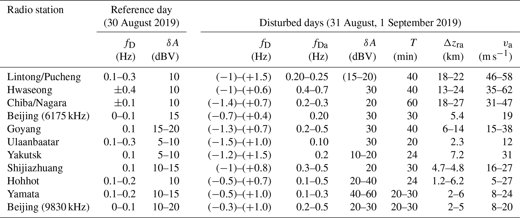
This system is located at the Harbin Engineering University campus in the People's Republic of China (45.78∘ N, 126.68∘ E; Chernogor et al., 2019a, b, c, 2020; Guo et al., 2019a, b, c, 2020; Luo et al., 2020a). The ionosphere is continuously monitored over 11 radio paths utilizing emissions from broadcasting stations in the 5–10 MHz frequency range and located in Japan, the Russian Federation, Mongolia, the Republic of Korea (South Korea), and the People's Republic of China (Fig. 1). The radio path lengths (Table 1) are found in the (1–2) × 103 km distance range, and the signal reception and processing is performed at the Harbin Engineering University.
Table 1Basic parameters of 11 radio paths used for probing the ionosphere at oblique incidence. Retrieved from https://fmscan.org/index.php (last access: 17 June 2021).
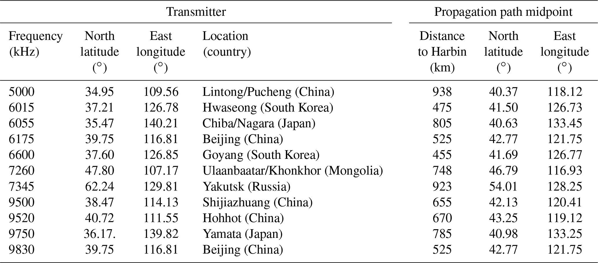
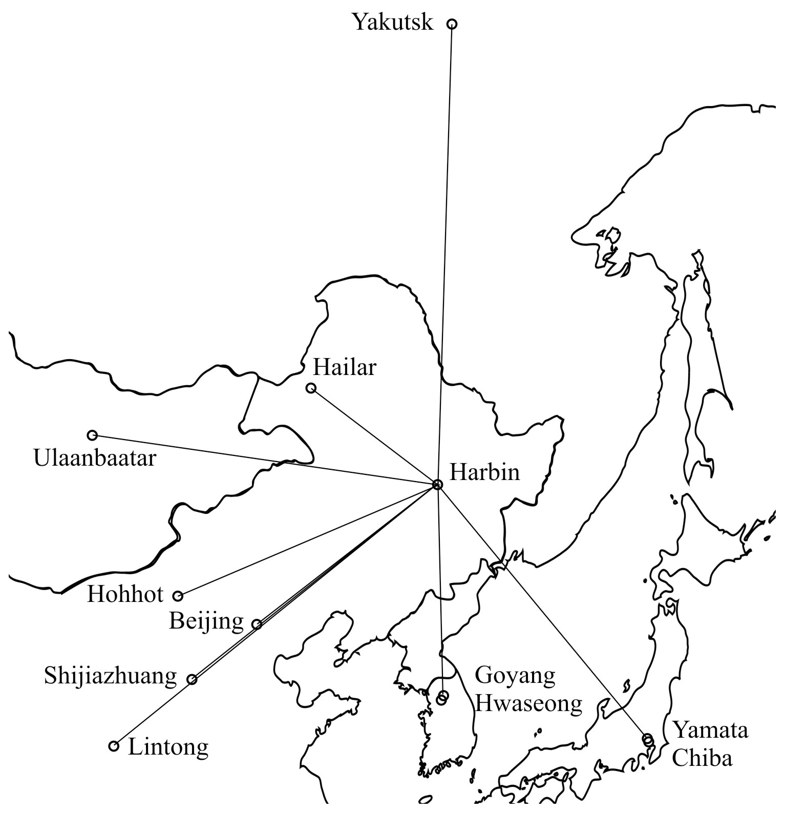
Figure 1Layout of the propagation paths used for monitoring dynamic processes acting in the ionosphere.
2.1.4 Ionosondes
Ionosondes are used to assess a general state of the ionosphere. The WK546 International Union of Radio Science (URSI) code ionosonde at the city of Wakkanai (45.16∘ N, 141.75∘ E), Japan, is the closest to Harbin (ionosonde stations in Japan can be found at https://wdc.nict.go.jp/IONO/HP2009/contents/Ionosonde_Map_E.html; last access: 15 June 2020). To assess the characteristic extent of the ionospheric storm, the city of Moscow's (the Russian Federation) ionosonde data are used (list of years for Moscow can be found at https://lgdc.uml.edu/common/DIDBYearListForStation?ursiCode=MO155; last access: 15 June 2020).
2.2 Analysis techniques
The fluxmeter magnetometer data recorded initially on a relative scale have been converted into absolute values using the magnetometer transfer function. Then, temporal dependencies of the geomagnetic field have been subjected to the systems spectral analysis, which simultaneously employs the short-time Fourier transform, the wavelet transform using the Morlet wavelet as a basis function, and the Fourier transform in a sliding window with a width adjusted to be equal to a fixed number of harmonic periods (Chernogor, 2008). Analysis of the obtained spectra follows.
The radio astronomy of the National Academy of Sciences of Ukraine three-axis fluxgate magnetometer has been used to control a general state of the geomagnetic field, and a specific signal processing procedure was not needed.
The data acquired by the multi-frequency multipath system for the oblique incidence radio sounding of the ionosphere have been subjected to processing in detail, and the products included the universal time dependencies of the Doppler spectra, the main ray amplitude, A(t), and the Doppler shift of frequency, fD(t). Furthermore, the fD(t) and A(t) were subjected to secondary processing to obtain the trends and , the fluctuations , , and the spectra in the period range T ≈ 1–60 min and greater (Chernogor, 2008).
The space weather variations under study are the event of corotating interaction region (CIR)/CH HS (where CH is coronal holes, and HS is high speed) origin combined with solar sector boundary crossing event, which could affect geomagnetic situation (see ftp://ftp.swpc.noaa.gov/pub/warehouse/2019/WeeklyPDF/prf2296.pdf, last access: 5 June 2020; Koskinen, 2011). The data retrieved from https://omniweb.gsfc.nasa.gov/form/dx1.html (last access: 18 June 2021) have been used to analyze the solar wind parameters. On 29 August 2019, the proton density, nsw, exhibited an increase from ∼106 to 15×106 m−3, and subsequently, a decrease from 15×106 to 1×10⁶ m−3 over the course of the next 3 d (Fig. 2). Over the course of 28 and 29 August 2019 and of the first half of 30 August 2019, the solar wind bulk speed, Vsw, varied from ∼350 to 500 km s−1. After 12:00 UT (universal time) on 30 August 2019 through about 01:00 UT on 1 September 2019, the Vsw value exhibited an increase from ∼400 to 750 km s−1, with a peak of 835 km s−1 observed early on 1 September 2019 (see ftp://ftp.swpc.noaa.gov/pub/warehouse/2019/WeeklyPDF/prf2296.pdf, last access: 5 June 2020). During almost 4 d, Vsw≈600–750 km s−1. Before 12:00 UT on 30 August 2019, the temperature, Tsw, of the solar wind particles was observed to be in the (1–2) × 105 K range. After 12:00 UT on 30 August 2019, it showed an increase from 105 to 4.4×10⁵ K in the course of 24 h, and eventually, fluctuating, it exhibited a gradual decrease from 4.4×10⁵ to 105 K. As expected, the increases in nsw and Vsw gave rise to an increase in the solar wind dynamic pressure, from ∼0.2 to ∼3 nPa. The east–west By and the north–south Bz components of the interplanetary magnetic field exhibited fluctuations in the −3 to 8 nT and −7 to 3 nT ranges, respectively. Since approximately 12:00 UT on 30 August 2019, the value of the Bz component remained predominantly negative. This indicated that the magnetic storm ensued. Over the following day (from 08:00 UT on 30 August 2019 to 07:00 UT on 3 September 2019), energy input per unit time, εA, from the solar wind into the Earth's magnetosphere occasionally increased to 14–15 GJ s−1; before the storm's commencement, the εA value did not exceeded 1 GJ s−1.
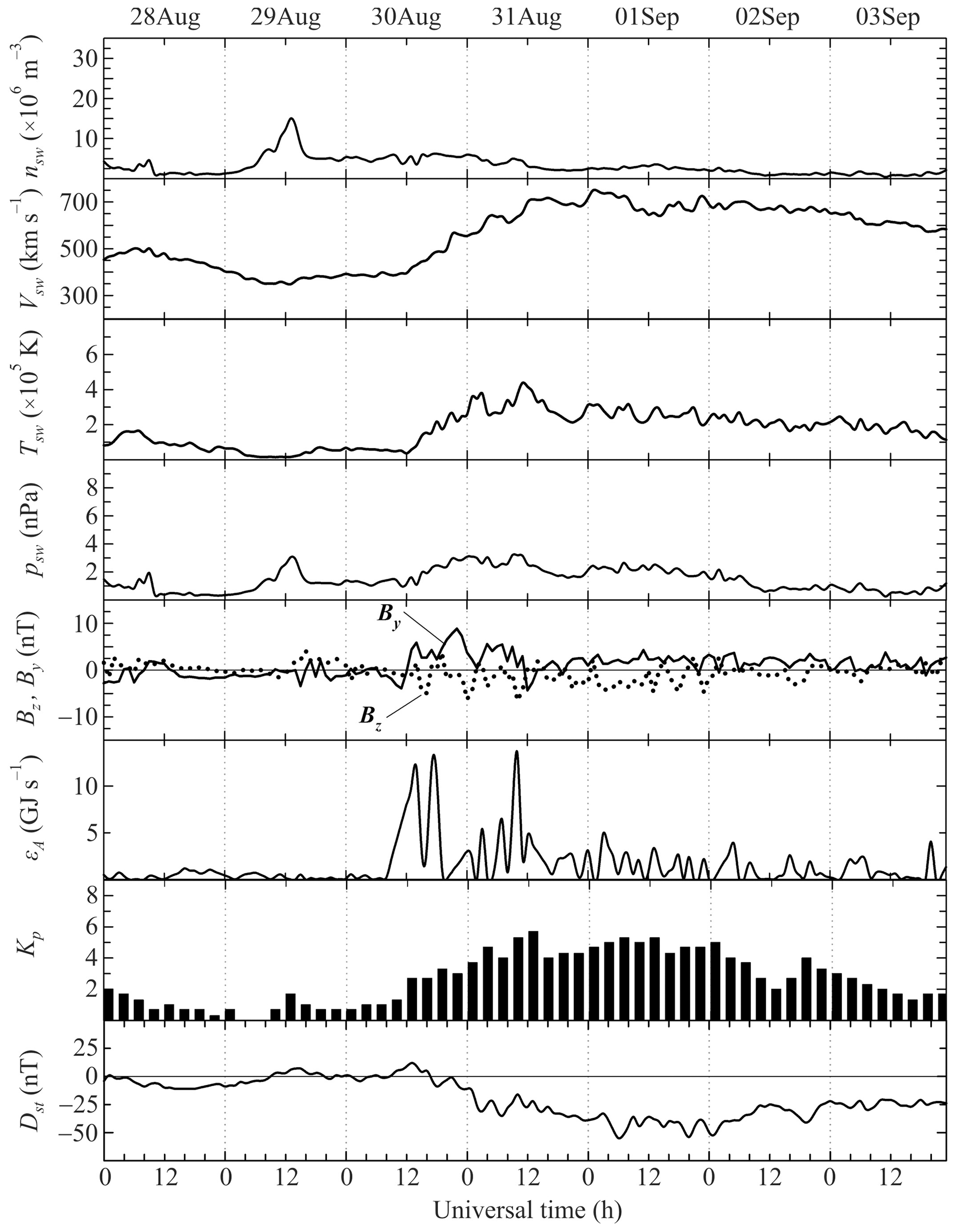
Figure 2Universal time dependencies of the solar wind parameters. Proton number density nsw, temperature Tsw, plasma flow speed Vsw (retrieved from https://omniweb.gsfc.nasa.gov/form/dx1.html, last access: 18 June 2021), calculated dynamic pressure psw, components Bz and By of the interplanetary magnetic fields (retrieved from https://omniweb.gsfc.nasa.gov/form/dx1.html, last access: 18 June 2021), and calculated energy input per unit time, εA, from the solar wind into the Earth's magnetosphere. Kp and Dst index (retrieved from https://omniweb.gsfc.nasa.gov/form/dx1.html, last access: 18 June 2021) for 28 August–3 September 2019 period. Dates are shown along the upper abscissa axis.
The Kp index values exhibited variations from 0 to 2 before the storm commencement and from ∼2 to 5.7 over 4 d afterwards. Before the storm commencement, the Dst index was observed to fluctuate in the −10 to 6 nT range. At about approximately 12:00 UT on 30 August 2019, Dst≈12 nT; from 10:00 to 14:00 UT, the storm commencement was observed to occur. After 20:00 UT on 30 August 2019, the Dst values began to show a gradual decrease to −55 nT, which was attained at about 06:00 UT on 1 September 2019; over this time period, the storm's main phase was observed to occur. After 06:00 UT on 1 September 2019, the storm transitioned to the recovery phase, which lasted for a few days. Thus, this magnetic storm was seen to be of quite a long duration over the last few years, but it was not the strongest, which is its main feature. A long duration ionospheric storm was expected to follow the longest duration magnetic storm. The geomagnetic and ionospheric storm features are described further in detail.
4.1 Level of geomagnetic field variations
Magnetic measurements at the Institute of Radio Astronomy of NASU Low Frequency Observatory, Ukraine (49.93∘ N, 36.95∘ E), show that the state of the geomagnetic field was quiet on 29 August 2019 (Fig. 3a). After 12:00 UT on 30 August 2019, relatively small, ∼10–20 nT, variations appeared in all geomagnetic field components (see Fig. 3b). On 31 August 2019, the variations increased up to 60–70 nT (see Fig. 3c). The Z component was changing less, by no more than 20 nT. The variations on 1 September 2019 remained approximately the same (see Fig. 3d). The fluctuation excursions of the components significantly decreased on 2 September 2019 (see Fig. 3e). Over the course of the next 2 d, the magnetic field remained weakly disturbed (see Fig. 3f); the fluctuation excursions did not exceed 15 nT (see Fig. 3f).
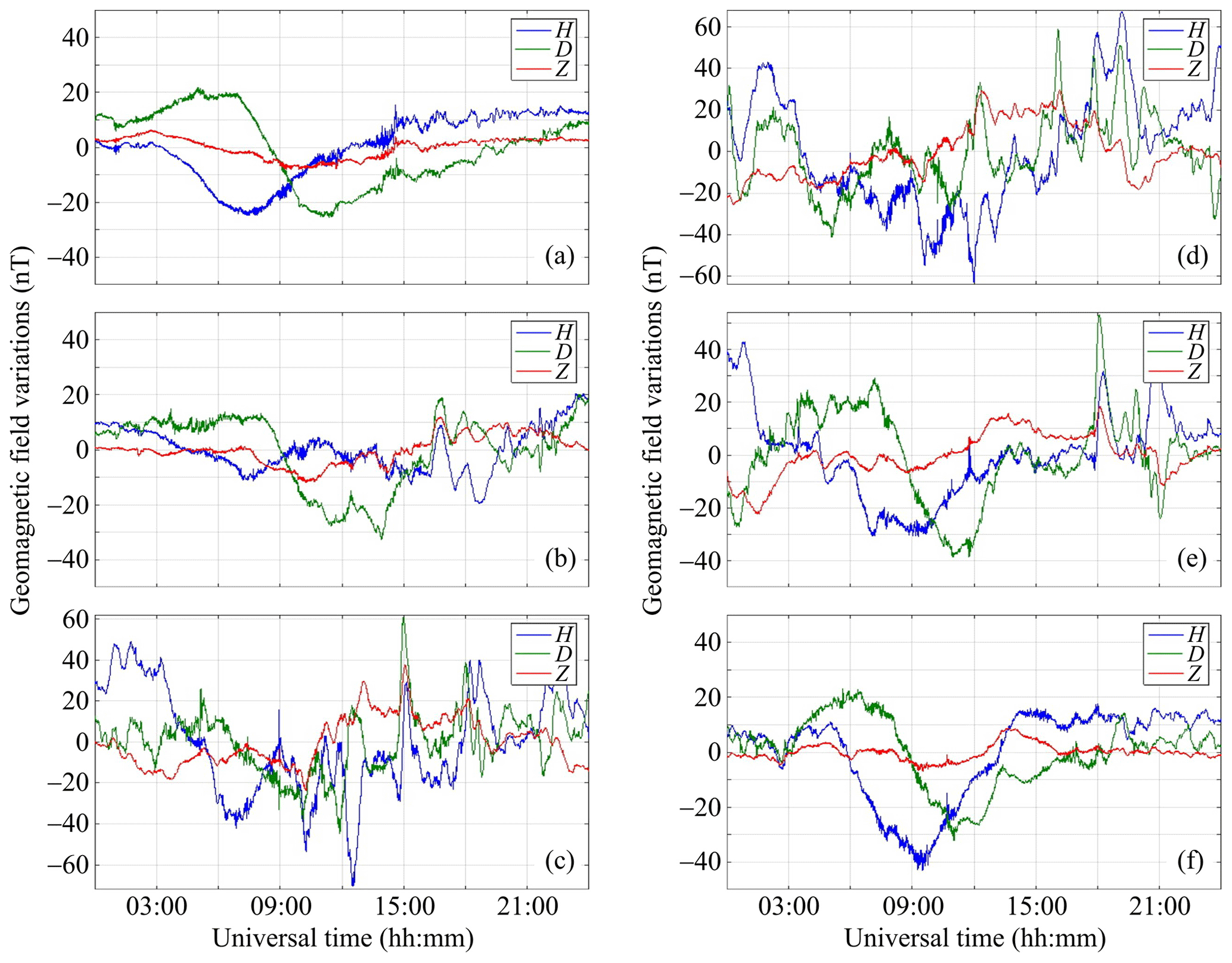
Figure 3H, D, and Z components for (a) 29 August 2019, (b) 30 August 2019, (c) 31 August 2019, (d) 1 September 2019, (e) 2 September 2019, and (f) 3 September 2019 (http://geospace.com.ua/en/observatory/metmag.html, last access: 18 June 2021).
4.2 Level of geomagnetic field fluctuations
Up to 11:00 UT on 29 August 2019, the variations in the geomagnetic field H and D components in the 1–1000 s period range at the V. N. Karazin Kharkiv National University Geomagnetic Observatory, Ukraine (49.65∘ N, 36.93∘ E), were insignificant at less than 0.2–0.3 nT (Fig. 4); from 11:00 to 17:00 UT, their level occasionally showed increases of up to ±1 nT. On 30 August 2019, approximately in the course of the sudden storm commencement, the level of fluctuations exhibited an increase by a factor of 2 to 3 times, which persisted for about 4–5 h. On 31 August 2019, in the course of the storm's main phase, the level of fluctuations showed an increase of up to 1.5–2 nT and, occasionally, even up to 4 nT. The duration of this effect was no less than 10 h.
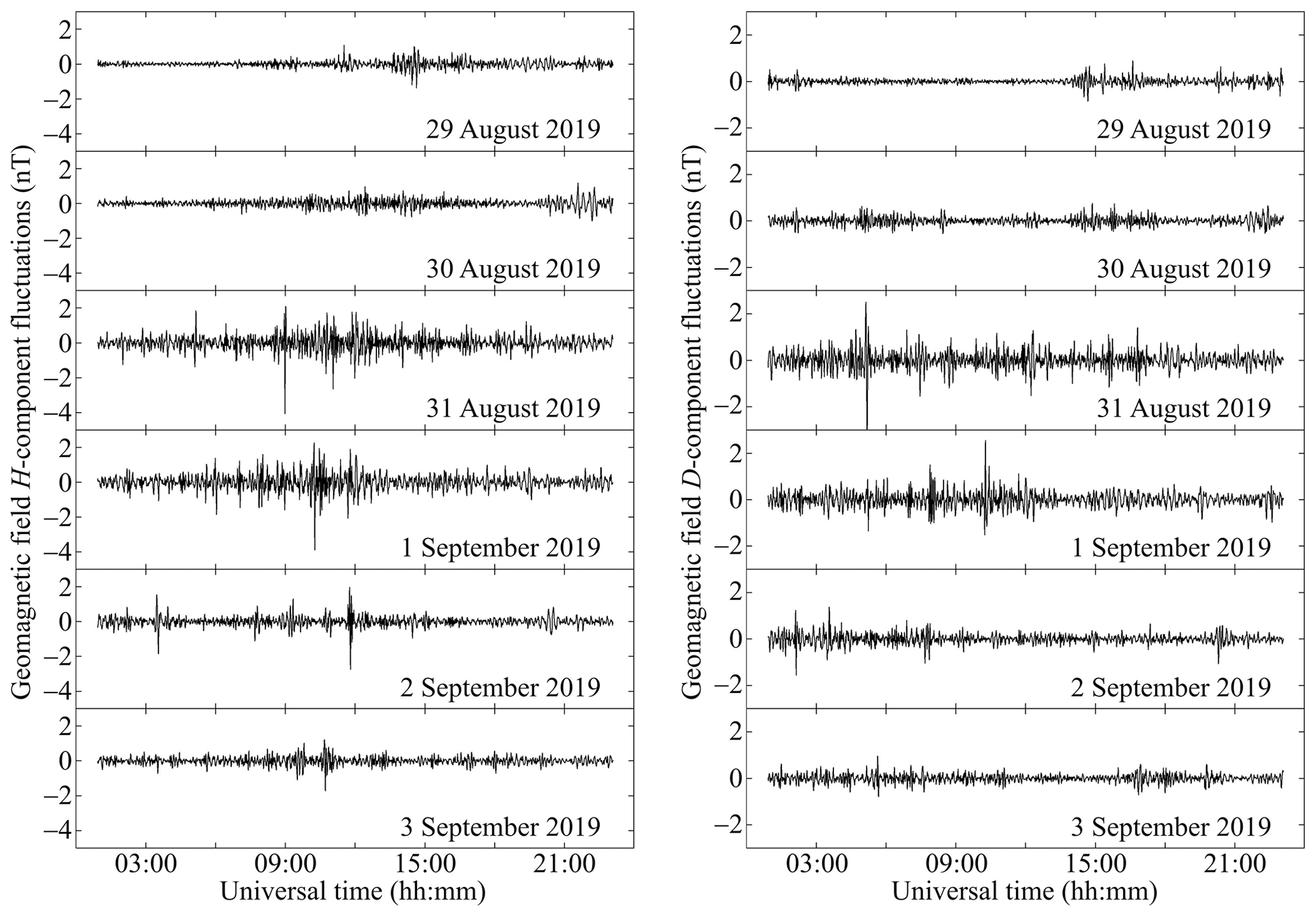
Figure 4Magnetic field variations at the V. N. Karazin Kharkiv National University Magnetometer Observatory.
On 1 September 2019, approximately from 08:00 to 13:00 UT, a considerable, up to 2–4 nT, increase in the level of fluctuations was also observed to occur. On 2 and 3 September 2019, the level of fluctuations also exhibited occasional enhancements of up to 1.5–2 nT that were approximately 1 h in duration.
The state of the ionosphere has been analyzed in general using the data from two ionosondes. The first of these is located in the vicinity of the propagation paths used for obliquely sounding the ionosphere, viz. near the city of Wakkanai (45.16∘ N, 141.25∘ E), Japan. To assess the characteristic extent of the ionospheric storm, ionosonde data from the city of Moscow (55.47∘ N, 37.30∘ E), the Russian Federation, have been used.
5.1 Data from ionosonde in Japan
Between 29 August and 3 September 2019, the minimum frequency, fmin, showed insignificant variations from 1.4 to 1.5 MHz. Only on 1 September 2019 was the fmin observed to exhibit spikes of up to 1.7–2 MHz.
The behavior of the E-layer critical frequency, , was observed to be approximately the same on all the days. During the daytime, this frequency attained 2.9–3.2 MHz; in the local evening, it decreased to 1.8 MHz; during the night, the was not observed, and in the course of 3 h in the morning, it showed an increase from 1.8 MHz to ∼3 MHz.
The sporadic E critical frequency, foEs, exhibited variations in a broad range of frequencies from ∼3 to ∼12–16 MHz. In the course of the storm's main phase, the foEs variations were insignificant.
Variations in the critical frequency, , of the F2 layer for the ordinary wave were observed to be small. During the daytime, this frequency was observed to be approximately 5 MHz, and during the night, it showed a gradual decrease from 4 to 3 MHz.
Generally, the universal time variations in the virtual height, , of the E layer were observed to be insignificant at a mere 5–10 km. However, approximately from 16:00 to 19:00 UT on 31 August and 1 September 2019, the height, , showed an increase from ∼100 to ∼120 km.
The sporadic Es layer virtual height exhibited considerable fluctuations from ∼80 to 160–170 km.
We have not succeeded in obtaining reliable data on the virtual height, , of the F2 layer. Most likely, it varied from 200 to 300 km.
5.2 Data from ionosonde at Moscow
The minimum frequency, fmin, values most frequently occurred in the 1.2–1.7 MHz range, and spikes of up to 2–3 MHz were observed only sometimes. From 07:30 to 08:30 UT on 31 August 2019, the fmin showed an increase from 1.4 to 2.2–2.4 MHz. During 1 through 3 September 2019, the fmin values exhibited considerable fluctuations.
The E layer critical frequency, , tracked the local time dependence of the electron density. The root mean square deviation did not exceed ∼0.1 MHz. In the daytime, the attained approximately 3 MHz; in the morning and in the evening, it showed an increase or a decrease of 1.3–1.4 MHz. Under nighttime conditions, we have not succeeded in measuring .
The sporadic E critical frequency, foEs, exhibited considerable fluctuations from 2 to 5–7 MHz. The fluctuation excursions in foEs under daytime conditions were observed to be greater than under nighttime conditions.
On 31 August 2019, from 05:00 to 08:00 UT, the foEs exhibited an increase from 3 to 6–7 MHz.
The critical frequency, , of the F2 layer for the ordinary wave showed a decrease to 3 MHz during the 28–29 August 2019 night, which was followed by an increase to 4.5 MHz during the daytime and even by an increase up to 5 MHz on 30 August 2019. During almost all local daytime on 31 August 2019, the was observed to be 0.7–1.1 MHz lower than on 29 August 2019. On 31 August 2019, from 09:00 to 11:00 UT and 12:00 to 15:00 UT, an increase in was observed to be 0.7–0.8 MHz. During the night and in the morning on 1 September 2019, the values were observed to be 0.5–0.6 MHz lower than those observed on 2 September 2019; during the daytime, the difference between these frequencies did not exceeded 0.2–0.3 MHz on average.
The virtual height, , of the E layer exhibited fluctuations in the 95–100 km range. On 31 August 2019, from 10:00 to 13:00 UT, it showed an increase from 102 to 113 km. A considerable increase in , from 110 to 133 km, also occurred at ∼ 12:30 UT on 1 September 2019.
The sporadic Es layer virtual height, , exhibited fluctuations in the 100–105 to 130–140 km range. On 31 August 2019, from 10:00 to 13:00 UT, this height showed an increase from ∼105 to 130 km. An increase from ∼110 to 125–132 km also took place on 1 September 2019 from 08:00 to 14:00 UT.
The virtual height, , of the F2 layer exhibited significant, from ∼200 to 400–500 km, fluctuations during the 29 August to 3 September 2019 period. Sharp, from 250 to 400–450 km, spikes in took place on 31 August 2019 during the 13:30–14:30 and 16:00–16:30 UT periods. Considerable, from 250–300 to 400–500 km, variations in were also observed to occur during the 31 August to 1 September 2019 night and from 16:00 to 18:00 UT on 1 September 2019.
6.1 Lintong/Pucheng to Harbin radio wave propagation path
The radio station operating at 5000 kHz is located in the People's Republic of China at a great circle propagation path range, R, of 1875 km from the receiver.
Approximately from 00:00 to 07:00 UT on 29 August 2019, i.e., during sunlit hours on the reference day, the signal amplitude, A, was observed to be dBV and the Doppler shift of frequency in the main ray signal, fD(t), to be ∼0.0 Hz, as can be seen in Fig. 5. After sunset at ∼ 07:00 UT, i.e., in the evening hours, the A showed a gradual increase of up to −40 dBV. The fD(t) values gradually decreased from 0 to −(0.5–1) Hz. Approximately from 09:00 to 16:00 UT, the Doppler spectra were observed to significantly broaden, from −2.5 to 2 Hz. On 30 August 2019, the fD(t) exhibited considerable, from −0.3 to 0.4 Hz, variations during the 18:00 to 22:00 UT period.
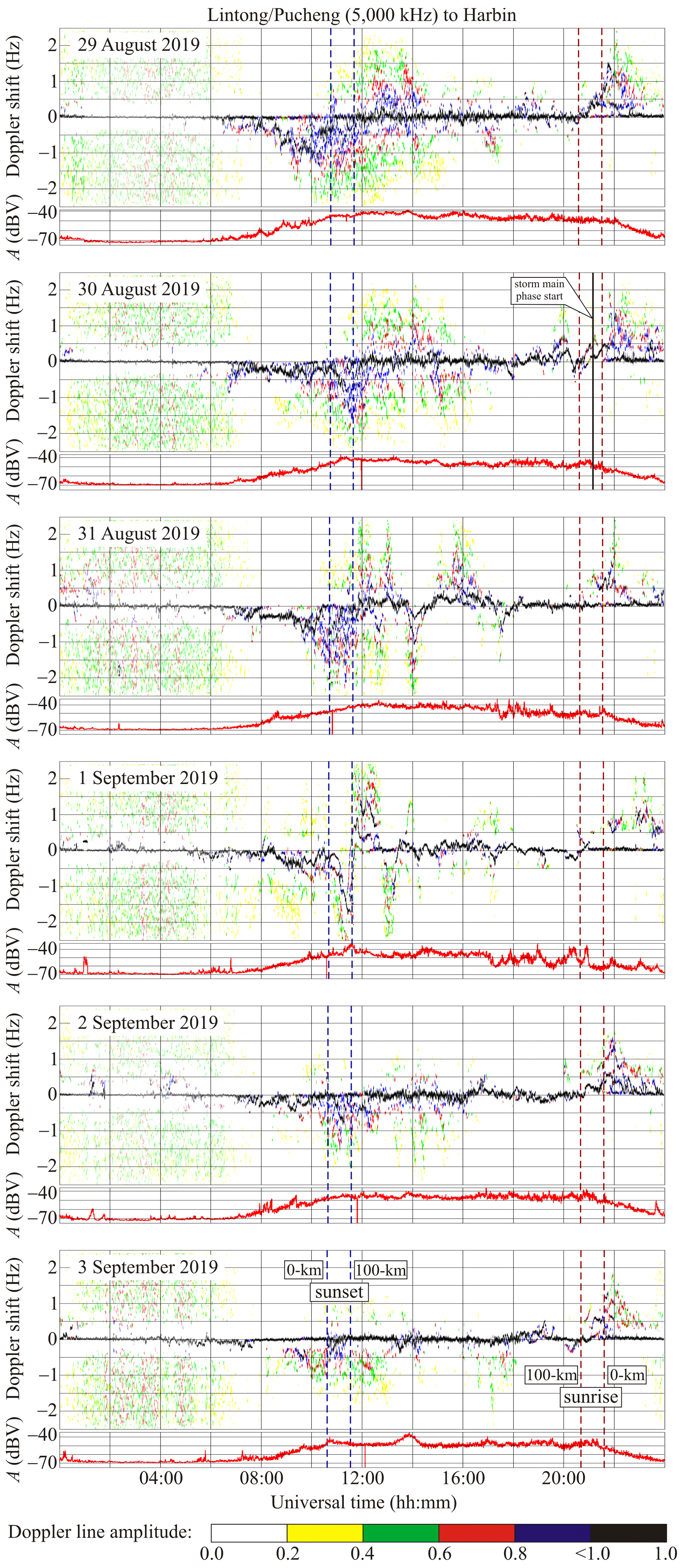
Figure 5Universal time variations in Doppler spectra and relative signal amplitude, A, along the Lintong/Pucheng to Harbin propagation path for 30 and 31 August and 1 and 2 September 2019 (panels from top to bottom). The radio wave frequency is 5000 kHz. The Doppler shift plot is comprised of 117 600 samples at every 1 h interval. The signal amplitude, A, at the receiver output in decibels, dBV, relative to 1 V is shown below the Doppler spectrum in every panel.
On 31 August 2019, the fD(t) changed from −0.3 to 0.3 Hz over the 12:00–18:00 UT period when quasi-periodic variations in the fD(t) took place in a ∼40 min period, T, and ∼0.20–0.25 Hz amplitude, fDa. From 17:00 to 22:00 UT, the amplitude A(t) exhibited considerable, up to 15–20 dBV, variations.
On 1 September 2019, the fD(t) showed a significant increase, from −1.8 to 1.4 Hz, in the course of sunset in the ionosphere. The ionospheric storm effect was observed to occur from at least 10:00 to 19:00 UT. The amplitude A(t) was observed to exhibit considerable, up to 20 dBV, variations during the 11:30–21:00 UT period. On 2 and 3 September 2019, the behavior of the Doppler spectra almost did not differ from that on the undisturbed day.
6.2 Hwaseong to Harbin radio wave propagation path
The 6015 kHz transmitter is located in the Republic of Korea at a ∼950 km distance from the receiver, and it did not operate from 00:00 to 03:40 UT.
On 29 August 2019, the Doppler shift of frequency fD(t)≈0 Hz occurred at almost all times (Fig. 6). The spectra were observed to exhibit maximum broadening near the dawn and dusk terminators. The variations in the signal amplitude represented the local time behavior.
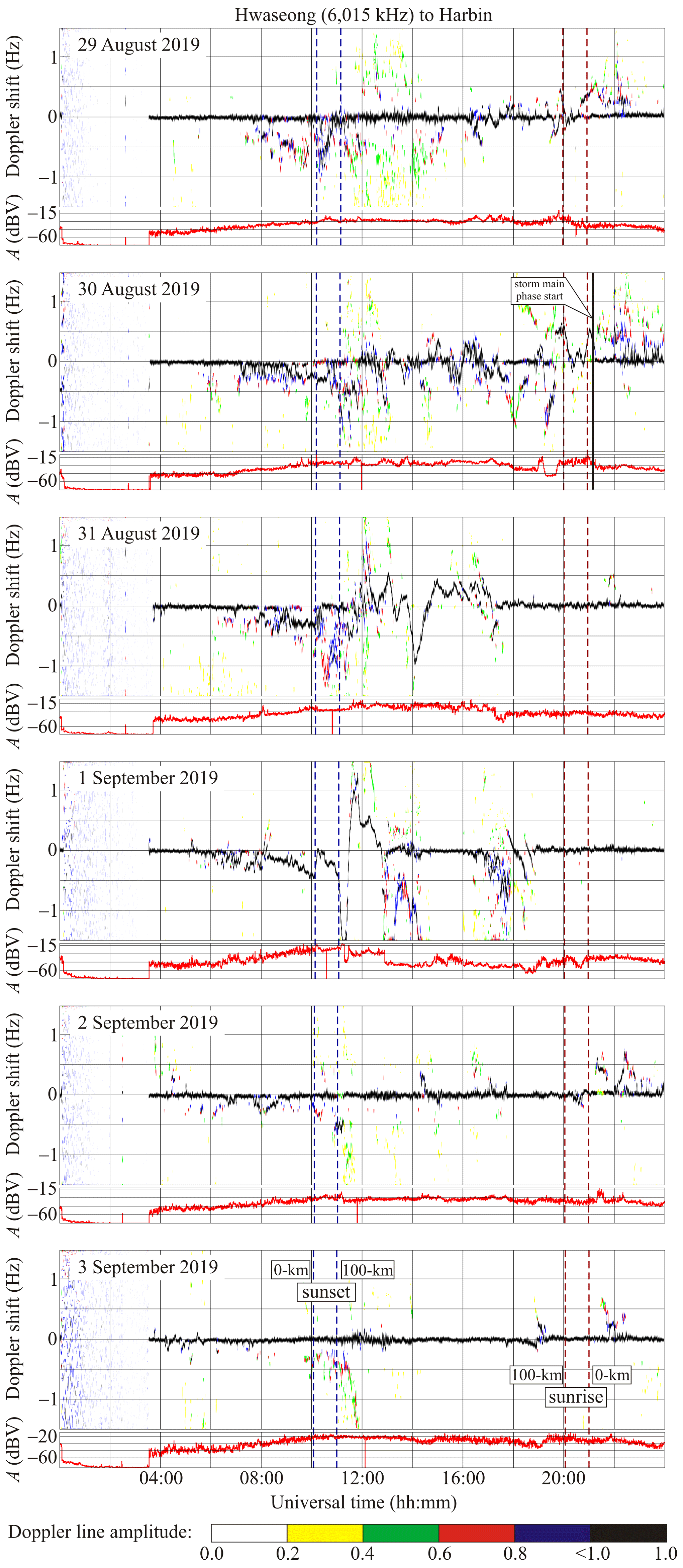
Figure 6Same as Fig. 5 but for the Hwaseong to Harbin radio wave propagation path at 6015 kHz.
On 30 August 2019, considerable (from −0.4 to 0.4 Hz) variations in the Doppler shift of frequency in the main ray were observed to occur from 13:00 to 21:00 UT with a ∼70–110 min quasi-period, T, and a ∼0.4 Hz amplitude, fDa.
On 31 August 2019, quasi-periodic changes in fD(t) were observed to occur from 12:00 to 17:00 UT with T≈40 min and fDa≈0.4–0.7 Hz.
On 1 September 2019, very significant (from −1.5 to 1.3 Hz) variations in fD(t) and the Doppler spectra took place from 10:00 to 14:00 UT and from 16:30 to 19:00 UT. From approximately 10:00 to 21:00 UT, large (up to 30 dBV) variations in signal amplitudes were evident.
On 2 and 3 September 2019, the Doppler spectra and signal amplitudes did not exhibit considerable variations.
6.3 Chiba/Nagara to Harbin radio wave propagation path
The radio station operating at 6055 kHz is located in Japan at a ∼1610 km range from the receiver. The signal transmissions were absent from 15:00 to 22:00 UT.
The Doppler spectra exhibited similar behavior on 29–31 August 2019 (Fig. 7). From 06:00 to 15:00 UT, the spectra were observed to be spread; they occupied the −1.5 to 1.5 Hz frequency range.
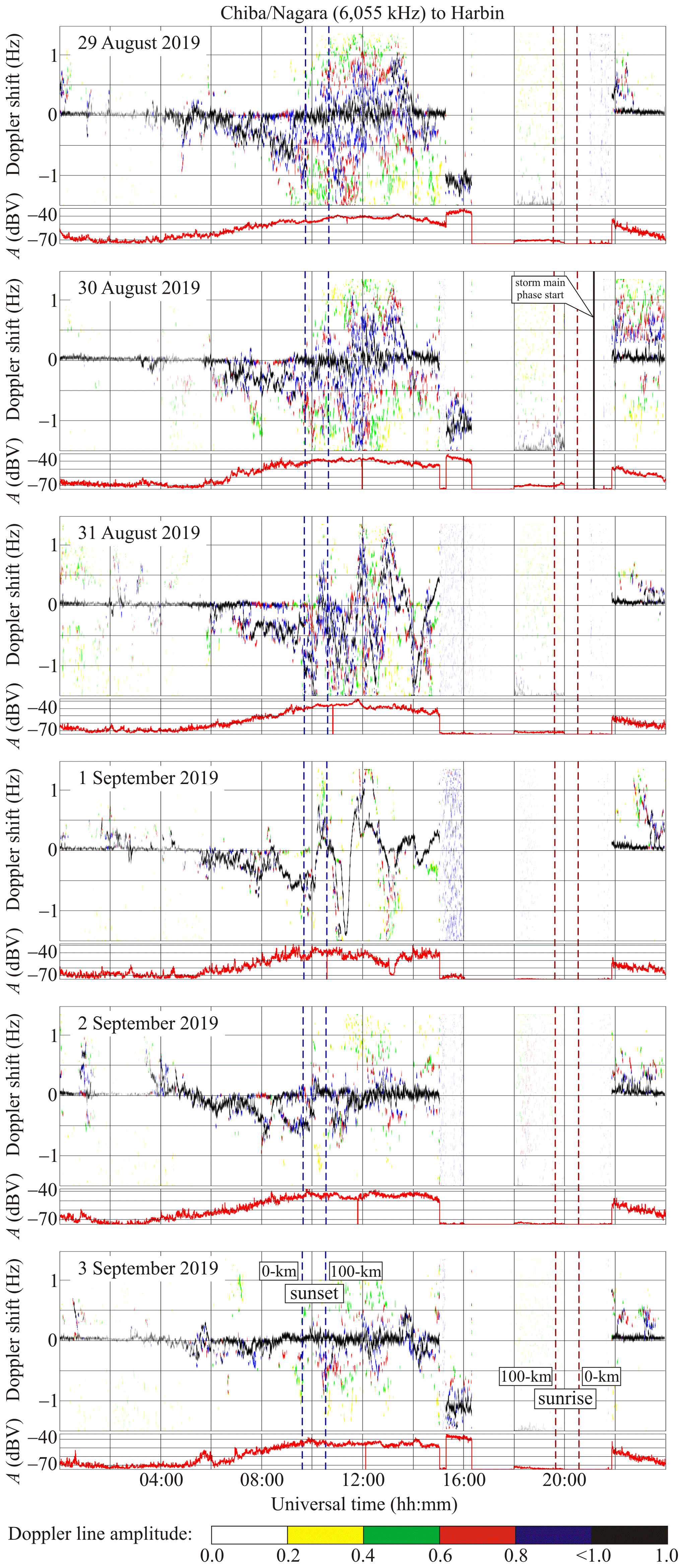
Figure 7Same as Fig. 5 but for the Chiba/Nagara to Harbin radio wave propagation path at 6055 kHz.
On 1 September 2019, the Doppler spectra exhibited behavior sharply different from that observed on the preceding day. The spread was evident weakly; from 10:00 to 15:00 UT, the Doppler shifts of frequency exhibited sharp changes from −1.5 to 1.3 Hz. The quasi-periodic process with the ∼60 min and greater period, T, and the ∼0.2 Hz and greater amplitude, fDa, became evident. On this day, the signal amplitude also exhibited considerable (up to 20 dBV) fluctuations.
On 2 September 2019, the Doppler spectra remained still disturbed over the 07:00–12:00 UT period.
On 3 September 2019, the Doppler spectrum spread was insignificant. The Doppler shift of frequency, fD(t), was observed to be close to the zero level most of the time.
6.4 Beijing to Harbin radio wave propagation path
The 6175 kHz transmitter is located in the People's Republic of China at approximately 1050 km range from the receiver. The transmitter operated only over the 09:00 to 18:00 UT and 20:20 to 24:00 UT periods.
On 29 and 30 August 2019, the Doppler spectra were characteristic of the single ray propagation; the second ray appeared only sporadically (Fig. 8). The Doppler shift of frequency, fD(t), was observed to be close to the zero level almost all the time, and the signal amplitude was dBV.

Figure 8Same as Fig. 5 but for the Beijing to Harbin radio wave propagation path at 6175 kHz.
On 31 August 2019, over the 12:00–18:00 UT period, the behavior of fD(t) sharply changed. The fD(t) dependence became quasi-periodic, with a ∼30 min period, T, and a ∼0.2 Hz amplitude. At approximately 14:00 UT, the fD dependence exhibited a sharp decrease from 0.2 to −0.7 Hz.
The fD was observed to exhibit considerable, from −1.2 to 1.1 Hz, variations over the 10:00–12:00 and 16:00–18:00 UT periods on 1 September 2019, while the signal amplitude showed a decrease of 30 dBV from 16:00 to 18:00 UT.
On 2 and 3 September 2019, the Doppler spectra exhibited the behavior characteristic of the quiet ionosphere.
6.5 Goyang to Harbin radio wave propagation path
The radio station operating at 6600 kHz is located in the Republic of Korea at a range, R, of ∼910 km from the receiver. From 05:00 to 08:50 UT, the Doppler measurements were neither possible over the entire measurement interval nor on 3 September 2019 during the 10:00–11:30 UT period.
On 29 August 2019, the Doppler spectra represented the undisturbed state of the ionosphere. For the main ray, the Doppler shift of frequency was fD(t)≈0 Hz (Fig. 9).
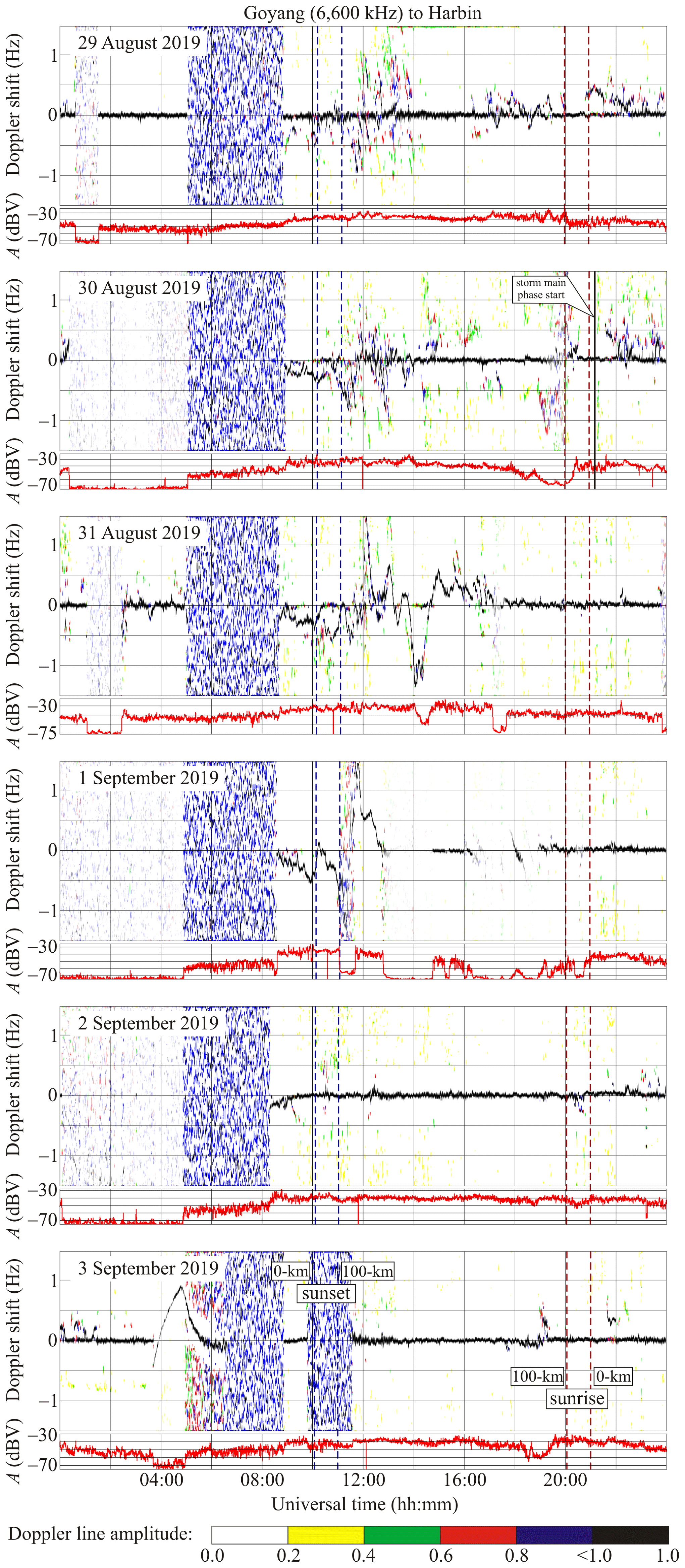
Figure 9Same as Fig. 5 but for the Goyang to Harbin radio wave propagation path at 6600 kHz.
On 30 August 2019, from 09:00 to 14:00 UT, the Doppler spectra showed a noticeable broadening. Over the same time period, the signal amplitude experienced an enhancement in fluctuations, attaining 15–20 dBV.
On 31 August 2019, from 09:00 to 17:00 UT, considerable, from −1.3 to 0.7 Hz, variations took place in the Doppler shift of frequency, fD(t). The variations in fD(t) were observed to be quasi-periodic, with ∼40 min periods, T, and ∼0.2–0.5 Hz amplitudes, fDa. From 17:30 to 19:00 UT, T≈15 min, and fDa≈0.1 Hz, the signal amplitude exhibited sporadic changes of up to 30 dBV.
On 1 September 2019, over the 08:30–13:00 UT period, the fD(t) also showed significant variations, from −1.5 to 0.7 Hz. The signal amplitude, A(t), fluctuated wildly, up to 30 dBV.
On 2 and 3 September 2019, the fD(t) and A(t) showed virtually no change. The state of the ionosphere along the propagation path was quiet.
6.6 Ulaanbaatar to Harbin radio wave propagation path
The radio station operating at 7260 kHz is located in Mongolia at a ∼1496 km range from the receiver. It was switched off from 05:00 to 07:00 UT and from 18:00 to 20:30 UT.
On 29 August 2019, the Doppler spectra showed that the propagation was more likely to occur along a single ray, and the fD(t) varied virtually monotonically (Fig. 10).
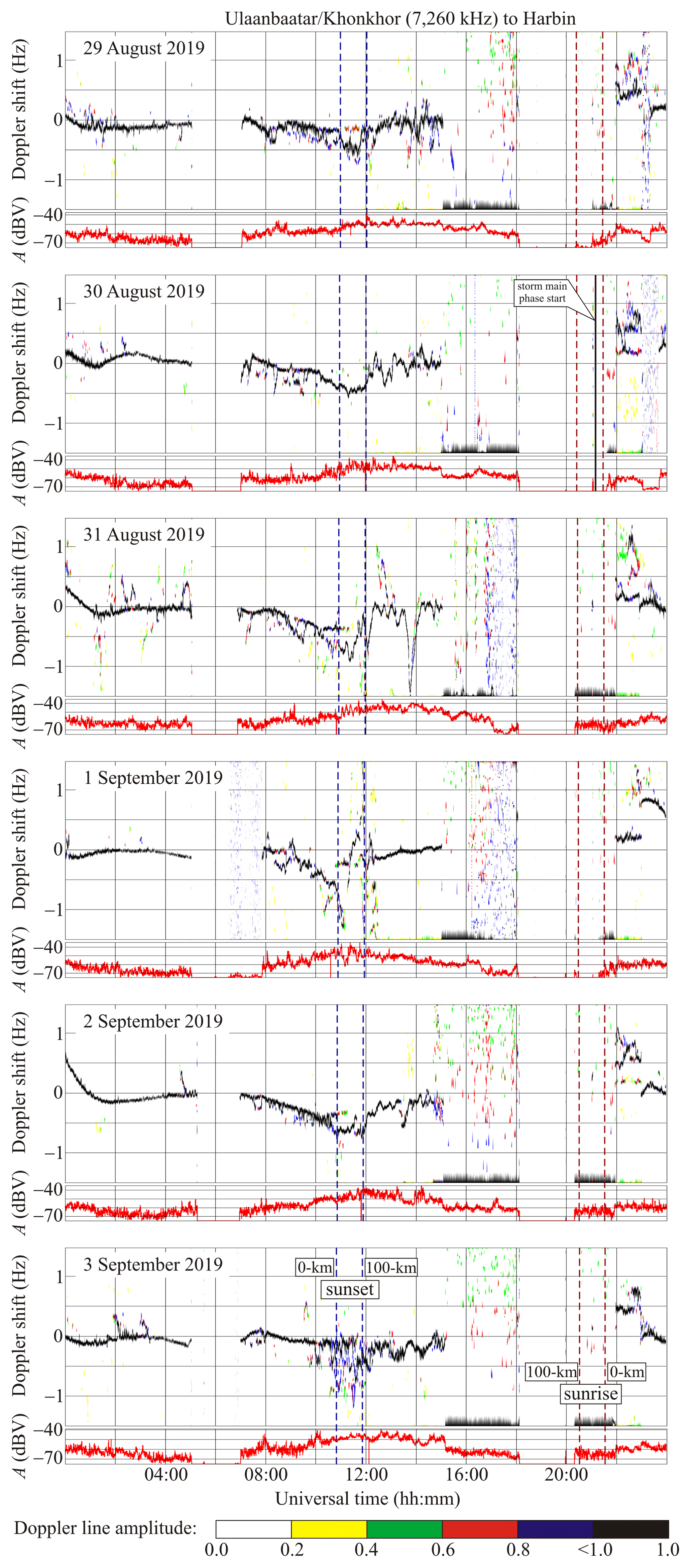
Figure 10Same as Fig. 5 but for the Ulaanbaatar/Khonkhor to Harbin radio wave propagation path at 7260 kHz.
On 30 August 2019, from 12:00 to 15:00 UT, the fD(t) exhibited quasi-periodic variations with 20 and 40 min periods, T, and with a ∼0.1 Hz amplitude, fDa, for T≈20 min and with fDa≈0.3 Hz for T≈40 min.
On 31 August 2019, the fD(t) fluctuated wildly and varied quasi-periodically with a ∼20 min period, T, and a ∼0.1 Hz amplitude, fDa, almost all the time. From 13:30 to 14:00 UT, it exhibited a sharp decrease from 0 to −1.5 Hz, which was followed by a subsequent increase from −1.5 to 0 Hz.
On 1 September 2019, during the 09:00–12:30 UT period, sharp changes in fD(t) became evident from 0 to −1.5 Hz and conversely.
On 2 September 2019, from 11:00 to 15:00 UT, the fD(t) exhibited quasi-periodic variations with a ∼20–25 min period, T, and a ∼0.1 Hz amplitude, fDa.
On 3 September 2019, from 13:00 to 15:00 UT, quasi-periodic variations in fD(t), with a ∼60 min period, T, and a ∼0.15 Hz amplitude, fDa, were also observed to occur.
From 30 August 2019 through 2 September 2019, an increase in the frequency and level of fluctuations in signal amplitude was noted.
6.7 Yakutsk to Harbin radio wave propagation path
The 7350 kHz transmitter is located in the Russian Federation at a range, R, of ∼1845 km from the receiver. Unfortunately, the transmitter operated only over the 11:00–18:00 and 20:15–24:00 UT periods.
On 29 and 30 August 2019, the Doppler spectra and signal amplitude exhibited relatively small variations (Fig. 11).
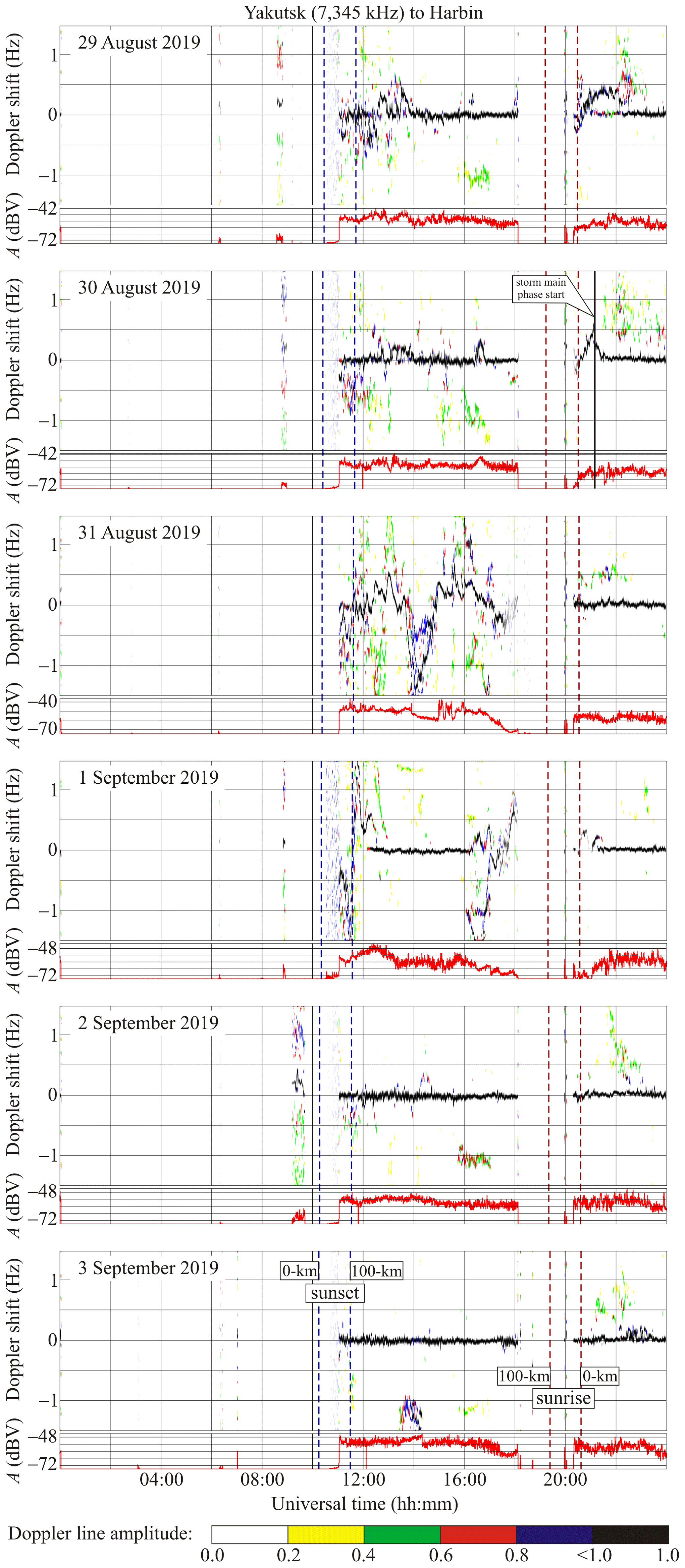
Figure 11Same as Fig. 5 but for the Yakutsk to Harbin radio wave propagation path at 7345 kHz.
On 31 August 2019, the Doppler spectra occupied the −1.5 to 1.5 Hz range. The fD(t) varied quasi-periodically with a ∼24 min period, T, and ∼0.2 Hz amplitude, fDa. From 13:40 to 14:50 UT, the fD(t) exhibited a decrease in fD(t) from 0 to −1.5 Hz, which was followed by an increase from −1.5 to 0 Hz, while the amplitude showed a decrease by 10 dBV. From 15:00 to 16:00 UT, the excursion of fluctuations in A(t) attained 20 dBV.
On 1 September 2019, the Doppler spectra and the signal amplitudes exhibited considerable variations during the 11:00–13:00 and 16:00–18:00 UT periods. From 16:00 to 18:00 UT, the spectra varied quasi-periodically, with 30–40 min periods, T, and 0.15 Hz amplitudes, fDa.
On 2 and 3 September 2019, the behavior of fD(t) and A(t) represented the behavior of the quiet ionosphere.
6.8 Shijiazhuang to Harbin radio wave propagation path
The radio station operating at 9500 kHz is located in the People's Republic of China at a ∼1310 km range, R, from the receiver.
On 29 and 30 August 2019, the behaviors of the Doppler spectra and signal amplitudes were similar. The ionosphere did not experience appreciable disturbances (Fig. 12).
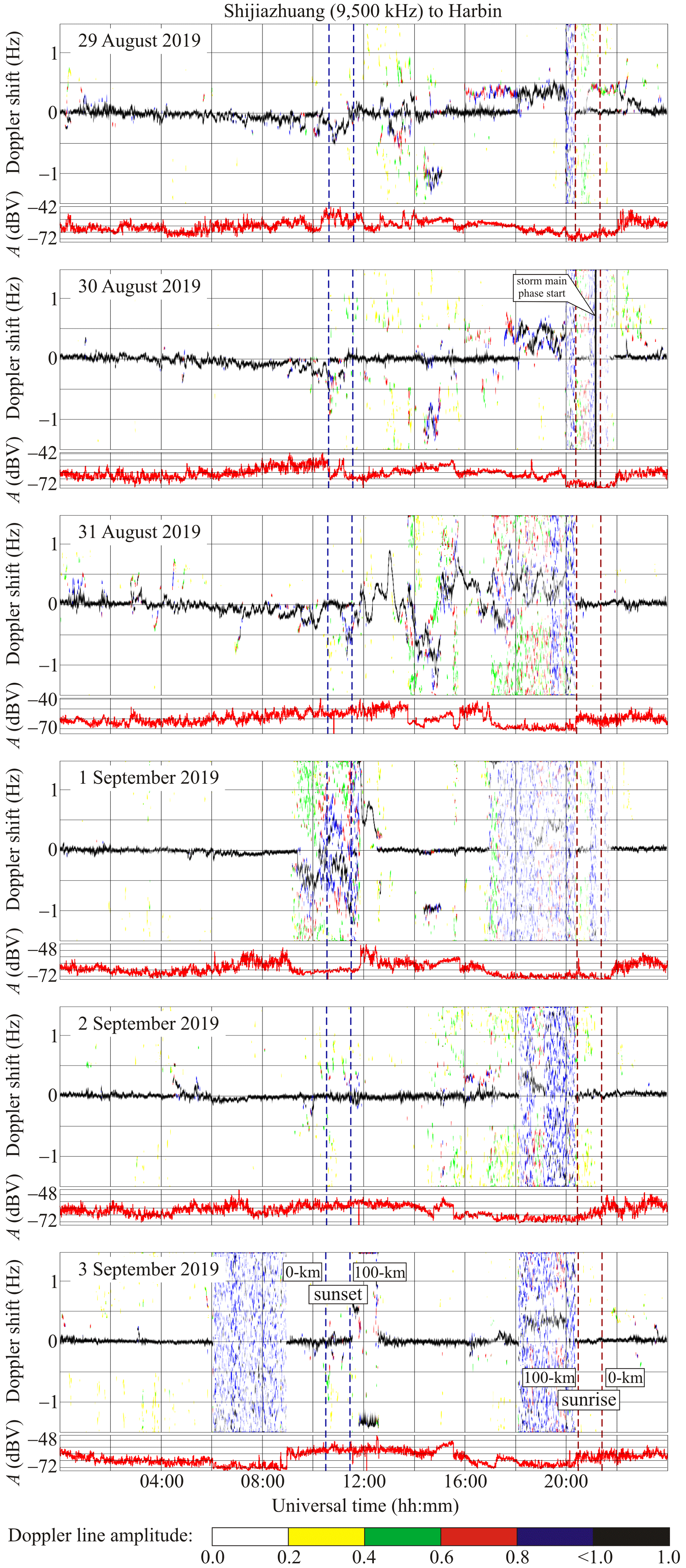
Figure 12Same as Fig. 5 but for the Shijiazhuang to Harbin radio wave propagation path at 9500 kHz.
On 31 August 2019, the Doppler spectra showed that the propagation is more likely to occur along a single ray. The fD(t) exhibited significant variations from −1 to 0.8 Hz. Quasi-periodic variations in fD(t), with a ∼30 min period, T, and a ∼0.3–0.5 Hz amplitude, fDa, became evident. From 17:00 to 20:25 UT, dBV, the signal amplitude was observed to be at the noise level. On 1 September 2019, the signal amplitude was also observed to be at the noise level during the 09:10–11:50 and 17:00–21:40 UT periods; during the rest of the time, fD(t)≈0 Hz.
The behavior of the Doppler spectra and the signal amplitudes on 2 and 3 September 2019 was characteristic of the undisturbed state of the ionosphere. Since fD(t)≈0 Hz all the time, the radio wave was apparently reflected from the Es-layer screening the ionospheric F region.
6.9 Hohhot to Harbin radio wave propagation path
The 9520 kHz transmitter is located in the People's Republic of China at a ∼1340 km range from the receiver. The radio station usually does not broadcast from 16:00 to 21:40 UT.
On 29 August 2019, considerable variations in the Doppler spectra, fD(t), and the signal amplitude, A(t), were observed to occur near the dusk and dawn terminators in the ionosphere (Fig. 13).
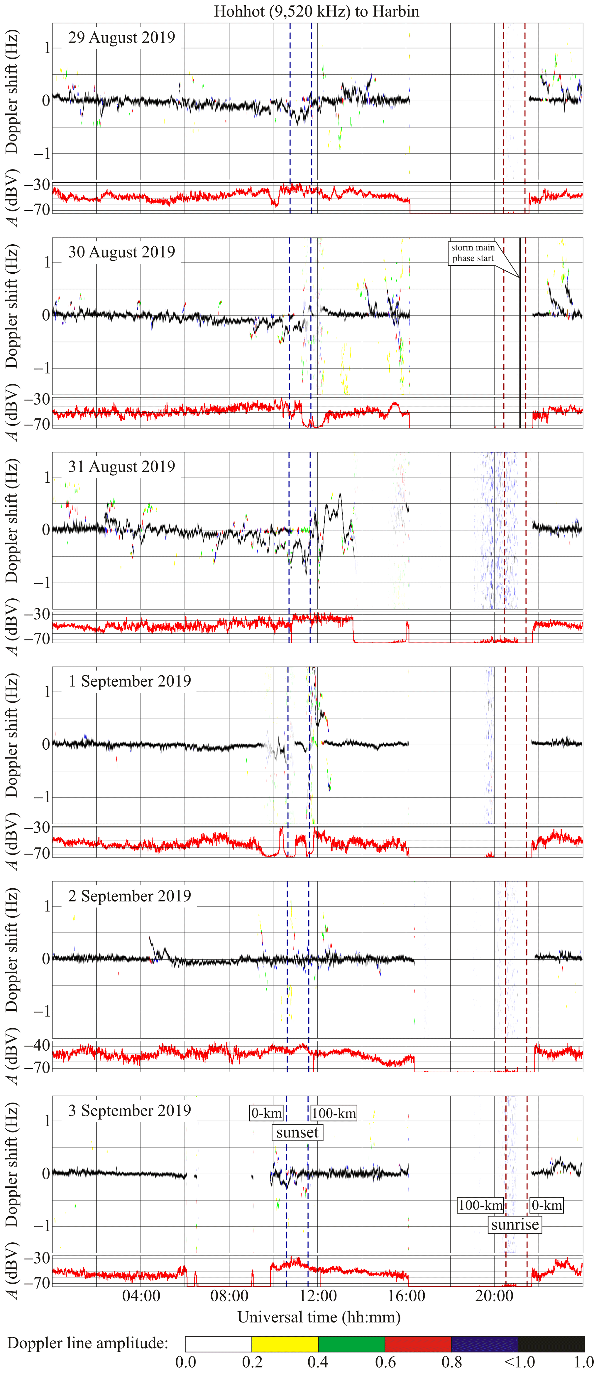
Figure 13Same as Fig. 5 but for the Hohhot to Harbin radio wave propagation path at 9520 kHz.
On 30 August 2019, significant variations in the Doppler spectra became evident from 14:00 to 16:00 UT.
On 31 August 2019, considerable, from −0.7 to 0.7 Hz, variations in fD(t) took place over the 11:00–13:30 UT period. The period, T, is observed to be ∼24 min, and the amplitude, fDa, is ∼0.1–0.5 Hz.
On 1 September 2019, fD(t)≈0 Hz almost all the time. Significant, 20–40 dBV, variations in A(t) were observed to occur from 08:00 to 16:00 UT.
On 2 and 3 September 2019, the ionosphere did not experience considerable disturbances.
6.10 Yamata to Harbin radio wave propagation path
The 9750 kHz transmitter is located in Japan at a ∼1570 km range, R, from the receiver. The transmissions are usually absent from 16:00 to 22:00 UT.
During the local daytime on 29–31 August 2019, the Doppler shift of frequency usually fluctuated around ∼0 Hz with periods, T, of about 20–30 min and amplitudes, fDa, of about 0.1 Hz (Fig. 14). From 10:00 to 14:00 UT, the Doppler spectra exhibited a significant broadening, and the fD(t) showed chaotic behavior.
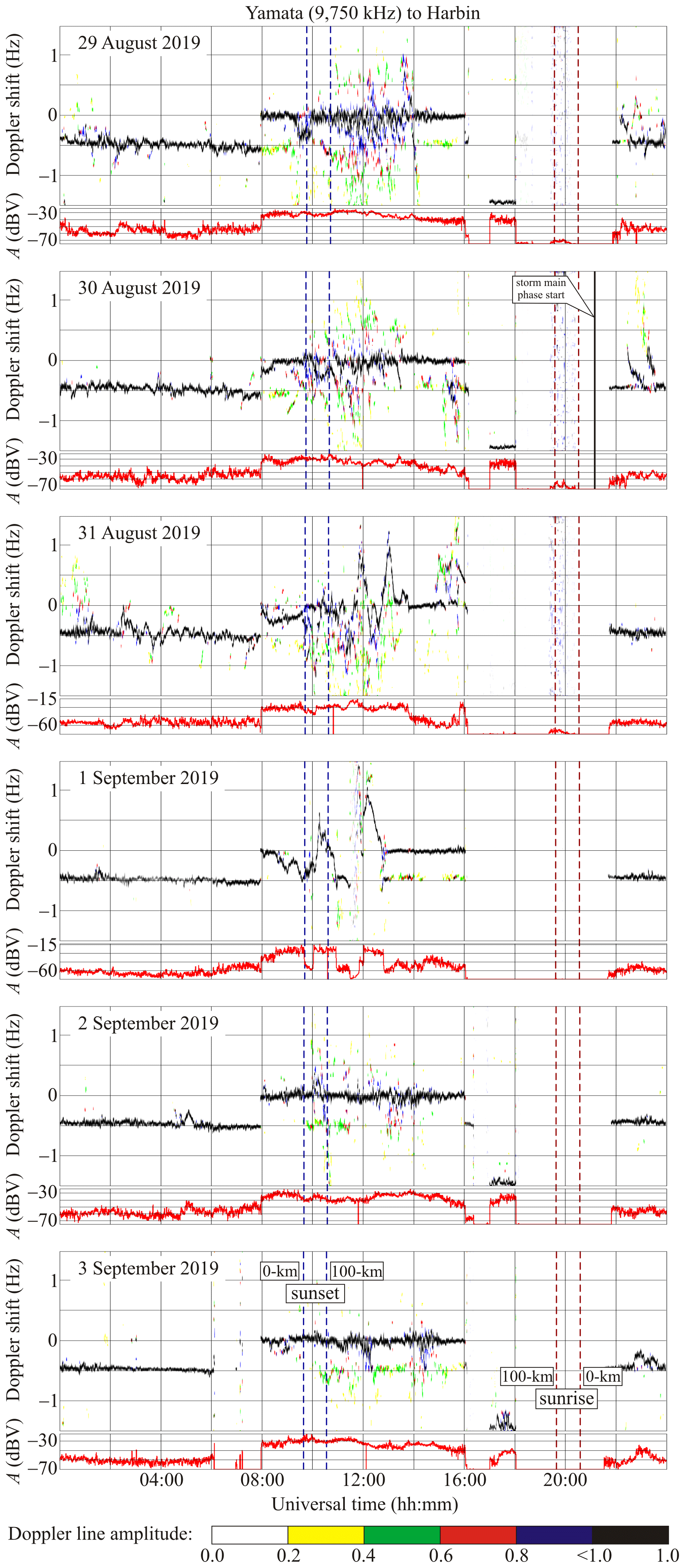
Figure 14Same as Fig. 5 but for the Yamata to Harbin radio wave propagation path at 9750 kHz.
On 30 August 2019, from 12:00 to 16:00 UT, the signal amplitude, A(t), exhibited near-quasi-periodic variations with a period, T, of about 30 min and 10–15 dBV excursions.
On 31 August 2019, a considerable, from −0.4 to 0.8 Hz, increase in variations in fD(t) was observed to occur from 12:00 to 16:00 UT, while the fluctuations in the signal amplitude, A(t), were small, in the 10–15 dBV range.
On 1 September 2019, the excursions in fD(t) varied from −0.5 to 1 Hz during the 08:00–13:00 UT period, while the signal amplitude exhibited sharp changes of 40–60 dBV.
On 2 and 3 September 2019, the fD(t) and A(t) exhibited behavior characteristic of the quiet days.
6.11 Beijing to Harbin radio wave propagation path
The radio station broadcasting at 9830 kHz over an interval shorter than half a day is located in the People's Republic of China at a ∼1050 km range, R, from the receiver.
On 29 and 30 August and on 2 and 3 September 2019, the Doppler spectra did not exhibit considerable variations (Fig. 15). Their variations were observed to occur from 11:00 to 16:00 UT on 31 August 2019 and from 10:00 to 12:30 UT on 1 September 2019.
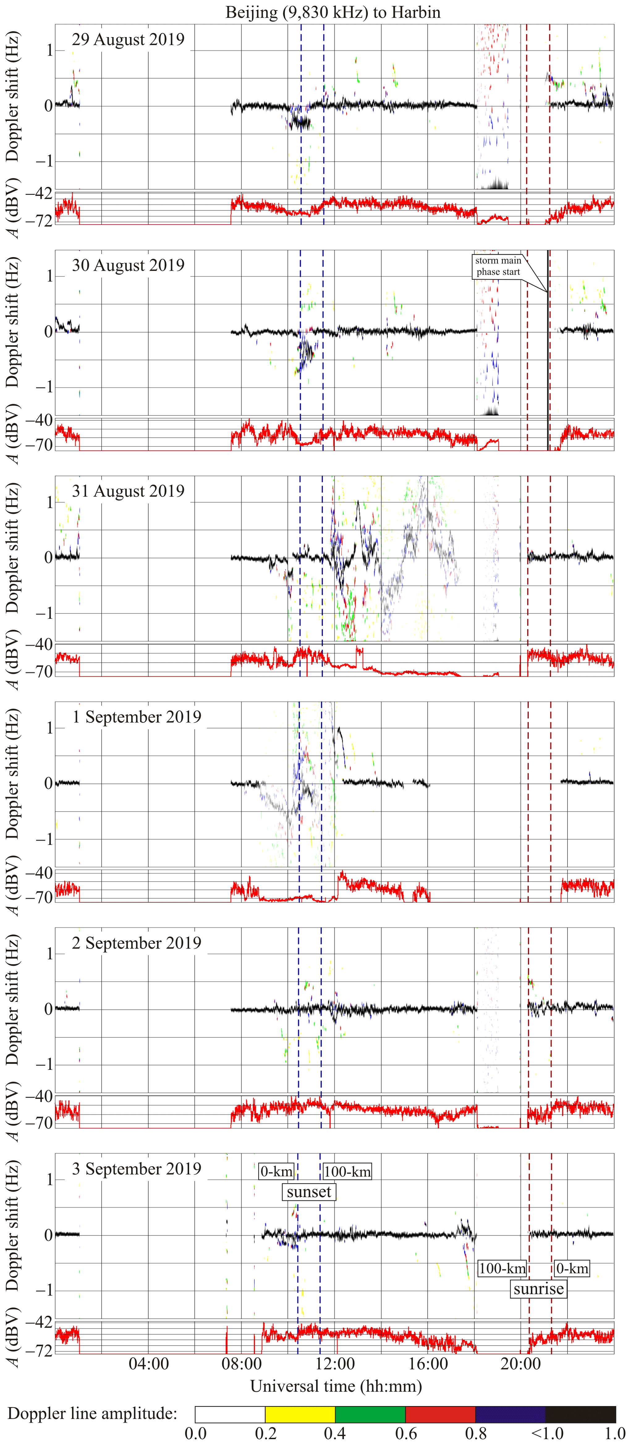
Figure 15Same as Fig. 5 but for the Beijing to Harbin radio wave propagation path at 9830 kHz.
On 30 and 31 August and on 1 September 2019, the signal amplitude exhibited considerable, up to 30 dBV, variations. The reflected signal was absent from 14:00 to 18:00 UT on 31 August 2019 and from 09:00 to 12:10 UT on 1 September 2019.
The strength of geospace storms is conveniently estimated by the energy entering the magnetosphere from the solar wind per unit of time, i.e., the Akasofu function. The index is defined as follows:
where GJ s−1 has been introduced in Chernogor and Domnin (2014) and is used to measure the storm strength. Substituting GJ s−1 for the storm under study gives Gst≈1.8. According to the classification of Chernogor and Domnin (2014), this storm is minor. Assuming the storm length to be Δt≈105 s, the energy entering the magnetosphere is found to be J. Such a storm falls under the Geospace Storm Index 1 (GSSI1) type (Chernogor and Domnin, 2014).
7.1 Geomagnetic field effects
The effects in the geomagnetic field began to appear after 12:00 UT on 30 August 2019. Considerable effects in the geomagnetic field occurred during the main phase of the magnetic storm, i.e., on 31 August and 1 September 2019. The recovery phase persisted for 2–3 d, from 00:00 UT, on 2 September 2019.
Let us estimate the magnetic storm energy Ems and the power Pms, using the following relation of Gonzalez et al. (1994):
where T is the equatorial magnetic induction, and J is the total energy in the Earth's dipole magnetic field.
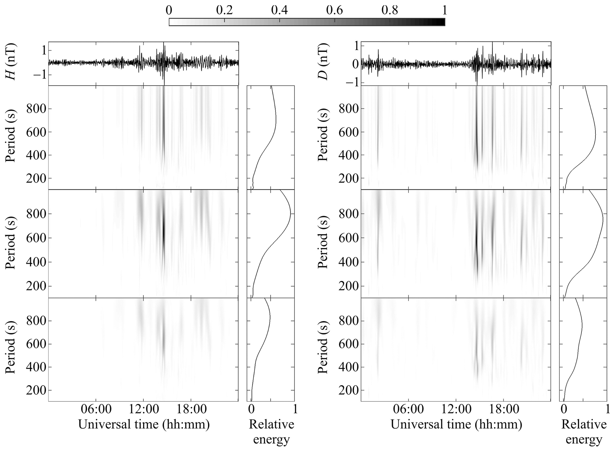
Figure 16Systems spectral analysis products for the geomagnetic variations on 29 August 2019 at the V. N. Karazin Kharkiv National University Magnetometer Observatory.
The corrected value of is given by the following:
where nT (J m, c=20 nT, , mp, and np are proton mass and number density, and Vsw is the solar wind bulk speed. Given nPa, nT, and nT, the magnetic storm energy is Ems=1.5 PJ. For the magnetic storm of 1.7×10⁵ s duration, the power is Pms≈9 GW.
In accordance with the NOAA (National Oceanic and Atmospheric Administration) Space Weather Scales (https://www.swpc.noaa.gov/noaa-scales-explanation last access: 18 June 2021), this storm is classified as moderate. In accordance with the classification system of Chernogor and Domnin (2014), magnetic storms with Kp=5.0–5.9 are classified as moderate, and their energy and power lie within the Ems≈(1–5)×1015 J and Pms≈(6–22)×1010 W limits, respectively.
7.2 Effects in geomagnetic field fluctuations
The universal time dependences of the horizontal components of the geomagnetic field in the 100–1000 s period range were subjected to the systems spectral analysis in the 100–1000 s period range.
The results of the spectral analysis for 29 August 2019, which could be considered as reference date, are presented in Fig. 16. The H- and D-component levels did not exceed 2–3 nT, while the spectra exhibited predominantly 600–900 s period oscillations.
On 31 August 2019, the day when the storm's main phase was observed, the H and D components attained 5–10 nT (Fig. 17). The spectra of the H and D components showed predominantly 300–400, 700–900 and 400–600 s, and 700–900 s period oscillations, respectively.
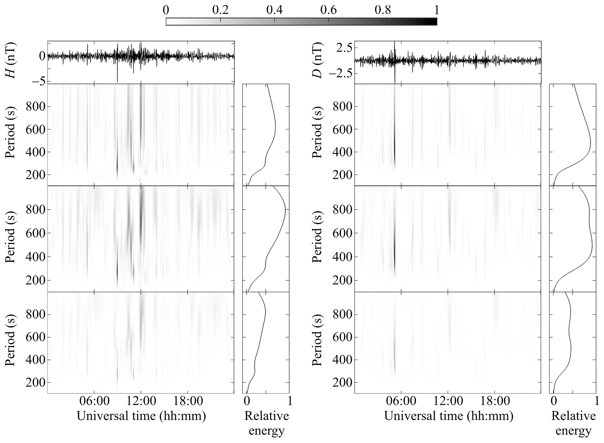
Figure 17Systems spectral analysis products for the geomagnetic variations on 31 August 2019 at the V. N. Karazin Kharkiv National University Magnetometer Observatory.
On 1 September 2019, the levels of the components remained the same as those on 31 August 2019. The 800–1000 s period oscillations were predominant in both components.
7.3 Ionospheric storm effects
7.3.1 Disturbances in ionogram parameters
Variations in ionogram parameters observed with the Japanese and Russian ionosondes exhibit similar behaviors. This suggests that the ionospheric storm under study is a large-scale phenomenon.
The list of the main effects that accompanied the ionospheric storm include the following:
-
an increase in fmin from 1.4 to 2.2–2.4 MHz between 07:30 and 08:30 UT on 31 August 2019;
-
an increase in from 3 to 6–7 MHz between 05:00 and 08:00 UT on 31 August 2019;
-
a decrease in by 0.7–1.1 MHz on 31 August 2019 compared to on 29 August 2019;
-
a decrease in by 0.2–0.6 MHz on 1 September 2019 compared to on 2 September 2019;
-
an increase in from 102 to 113 km between 10:00 and 13:00 UT on 31 August 2019;
-
an increase in from 110 to 133 km at approximately 12:30 UT on 1 September 2019;
-
an increase in from 105 to 130 km between 10:00 and 13:00 UT on 31 August 2019;
-
an increase in from 110 to 125–132 km between 08:00 and 14:00 UT on 1 September 2019;
-
brief spikes in from 250 to 400–450 km between 13:30 and 14:30 UT and between 16:00 and 16:30 UT on 31 August 2019;
-
an increase from 250–300 to 400–500 km during the 31 August–1 September 2019 night and between 16:00 and 18:00 UT on 1 September 2019.
Analysis of the ionograms indicates that the ionospheric storm occurred mainly during the 31 August and 1 September 2019 period. The storm duration virtually coincides with the duration of the magnetic storm's main phase.
Since the values on 31 August 2019 were less than those on 29 August 2019, a reference day, by 0.7–1.1 MHz, the ionospheric storm should be classified as negative. Furthermore, the values on 1 September 2019 were less than those on 2 September 2019, which is another reference day.
An estimation of a decrease in the electron density, N, during the ionospheric storm compared to the electron density, N0, on the reference day has been made using the following relation:
The dawn, daytime, and dusk ratio for 31 August 2019 were observed to be 1.8–2, 1.4, and 2.4, respectively.
The dawn and daytime ratio for 1 September 2019 was observed to be close to 1.56 and 1.16, respectively.
Given the , the negative ionospheric index (Chernogor and Domnin, 2014) can be calculated as follows:
For this storm, and INIS≈3.8 dB. In accordance with the Chernogor and Domnin's (2014) classification, the strength of such an ionospheric storm is classified as being negative ionospheric storm index 3, NIS3. Furthermore, this geospace storm manifested itself not only in the ionospheric F region but also in the ionospheric E region and in the sporadic Es layer.
As a whole, the mechanisms for negative ionospheric storms are well known. They include an enhancement in the wind speed, traveling atmospheric disturbances propagating equatorward (Prölss, 1993a, b), composition changes in the thermosphere, and an increase from ∼0.1—0.3 to 5–10 mV m−1 in an eastward zonal electric field arising during an electrical storm (see Sect. 1) that acts to decrease the electron density and increase the F2 layer virtual height.
The estimate of the ionospheric storm index and of the energy of the geospace and magnetic storms have allowed us to establish that a weak geospace storm acted to give rise to a moderate magnetic storm and to a strong ionospheric storm, which is not as trivial as may be supposed. The establishment of this fact would be impossible without the quantitative estimates.
During ionospheric storms, the phases/ionospheric response (positive and negative) are usually alternating. In most cases, the CIR storms have positive effect just after storm onset. Storms are usually accompanied by large- or medium-scale traveling ionospheric disturbances formed by gravity waves (GWs) that propagate from high latitudes toward the Equator.
7.3.2 Radio wave reflection height variations
The ionosonde data show that the virtual reflection heights , , and exhibit sharp, brief spikes at particular times. This suggests that significant changes are occurring in the N(h) profile. The variations in N(h) acted to change the Doppler shift of frequency fD(t) sharply. On 31 August 2019, at about 14:00 UT, the fD, virtually along all propagation paths, exhibited a sharp decrease from 0 to −(1–1.5) Hz, followed by an increase from the minimum value to 0 Hz. This duration of this effect was observed to be 50 to 60 min for different propagation paths. The sharp decrease in fD(t), followed by its increase to the initial value, indicates that a rise in the reflection height occurred. A rise in the altitude can be estimated by using the following simplified relation:
where c is the speed of light, ΔfDm is a fD maximum value, ΔT1 is the duration of a decrease in fD(t), ΔT is an overall duration of the variation in fD, and and are values averaged over ΔT1 and ΔT−ΔT1, respectively; θ is an angle of incidence with respect to the vertical.
Often, , i.e., . Hence, from Eq. (1), one has the following relation:
where, the following designation is used:
Then it follows, from Eqs. (1) and (2), that the altitude of reflection increases when ΔfDm<0 and vice versa.
The expression in Eq. (2), when applied to the Lintong/Pucheng–Harbin propagation path, where Hz and ΔT=60 min for nighttime conditions, gives Δzr≈110 km, i.e., the altitude exhibits an increase from ∼150 to ∼260 km. For the Hwaseong–Harbin propagation path, where Hz and ΔT≈60 min, the level of reflection shifts upward in altitude from 150 to 300–310 km. Regarding the mechanism for an increase in the height of reflection from 150 to 300 km, such a large increase was observed at one time, 14:00 UT on 31 August 2019, when a few causes merged together. First, the rearrangement of the evening ionosphere into the night ionosphere had been completed, which was accompanied by a decrease in the electron density and an increase in the height of reflection. Second, due to the processes referred to above, the negative ionospheric storm ensued. Third, a large negative half-wave of the quasi-periodic disturbance had arrived, which was observed along all radio wave propagation paths from about 12:00 to 16:00 UT. Variations in the height of reflection that occurred over other time intervals were observed to occur within the 30–50 km limits.
The altitudes of reflection along other propagation paths were estimated to be of the same order of magnitude. This effect is also a manifestation of the ionospheric storm.
7.3.3 Wavelike disturbance effects
The ionospheric storm was accompanied by the generation of quasi-periodic variations in the Doppler shift of frequency. From 12:00 to 17:00 UT on 31 August 2019, virtually all propagation paths exhibited a quasi-periodicity in fD(t) at the ∼30 min period, T, and ∼0.4–0.6 Hz amplitude, fDa. Given the fDa, the amplitude of variations in the electron density can be estimated by employing the following relation (Guo et al., 2019a, 2020; Chernogor et al., 2020):
where , , , , zr is the altitude of reflection, r0 is the Earth's radius, H is the scale height of the atmosphere, and Ln is a characteristic scale length of changes in the refractive index in the ionosphere.
The expression in Eq. (3) suggests the following:
where z0 is a reference height, e.g., 100 km.
Applying the expression in Eq. (3) to, for example, the Hwaseong–Harbin propagation path, where zr≈150 km, fDa=0.4 Hz, T=30 min, and L≈30 km, yields δNa≈42 %. Along the Goyang–Harbin propagation path over the 17:30–20:00 UT period, an oscillation with a ∼15 min period, T, and 0.1 Hz amplitude, fDa, was observed to occur. Substituting zr≈200 km and L≈80 km in Eq. (3) leads to δNa≈6 %.
Table 2Aperiodic variations in the signal amplitude, δA, and aperiodic and quasi-periodic variations in the Doppler shift of frequency, together with fD, with amplitude fDa and period T, and the amplitudes of variations in the level of reflection, Δzra, and in the speed of the level of reflection, va.
The magnitudes of periods of ∼15–60 min and of the amplitudes δNa suggest that the quasi-periodic variations in fD(t) and N(t) launched atmospheric gravity waves (AGWs). It is well known that AGWs are generated in the auroral oval in the course of geospace storms and propagate to low latitudes (see, for example, Hajkowicz, 1991; Lei et al., 2008; Lyons et al., 2019). We have tried to find a confirmation of this fact in our measurements. For example, the minimum magnitude of the Doppler shift of frequency along the Ulaanbaatar to Harbin (7260 kHz) propagation path is observed to occur at approximately 12:47 UT and along the Beijing to Harbin (6175 kHz) propagation path at 13:00 UT. Taking into account the distance of 400 km between the propagation path midpoints in the equatorward direction yields the equatorward speed of 510 m s−1. Such speeds and periods of tens of minutes are inherent in atmospheric gravity waves. Thus, the generation of AGWs responsible for traveling ionospheric disturbances is also a manifestation of geospace storms.
7.3.4 Variations in radio wave characteristics
Ray tracing has shown that radio waves at frequencies equal to ∼5–10 MHz were reflected from the ionosphere during the daytime at relatively low altitudes (z≈100–150 km), where the electron density was perturbed by the geospace storm relatively weakly, and the variations in fD usually did not exceed 0.1–0.2 Hz on both quiet and disturbed days. Under nighttime disturbed conditions, the altitude of reflection increased by 120–220 km, and the Doppler shift of frequency, fD, exhibited significant aperiodic variations from −1.5 to +1.5 Hz and somewhat smaller (see Table 2). In contrast, during quiet days, such variations usually did not exceed ± (0.1–0.3) Hz. On 31 August and 1 September 2019, the quasi-periodic variations in the Doppler shift of frequency was observed to occur during the night with amplitude, fDa, of 0.2 to 0.5 Hz and a period of 24 to 60 min (see Table 2), while the level of reflection oscillated with an amplitude of ∼10 to ∼20–30 km and traveled with a velocity of ∼10 to ∼60 m s−1. Table 2 shows that the amplitude variations on the disturbed day were considerably greater than the variations on the quiet day.
The studies presented at this paper demonstrate conclusively that the multi-frequency multipath facility involving the software-defined technology for obliquely sounding the ionosphere at the Harbin Engineering University is an effective means for investigating the influence of ionospheric storms on the characteristics of HF radio waves and the short-term variability of dynamic processes operating in the ionosphere.
-
The energy and power of the geospace storm have been estimated to be 1.5×10¹⁵ J and 1.5×10¹⁰ W, which means that this storm is classified as weak.
-
The energy and power of the magnetic storm have been estimated to be 1.5×10¹⁵ J and 9×10⁹ W, which means that this storm is classified as moderate. The storm's main feature is its main phase duration of up to 2 d. The recovery phase was also long, at no less than 2 d.
-
Over the course of 31 August and 1 September 2019, the H- and D-component disturbances attained 60–70 nT. The Z-component variations did not exceed 20 nT.
-
On 31 August and 1 September 2019, the level of fluctuations in geomagnetic field in the 1–1000 s period range exhibited an increase from 0.2–0.3 to 2–4 nT. The oscillations in the range from the 300–400 to 700–900 s period had maximum energy.
-
During the geospace storm, a moderately to strongly negative ionospheric storm was manifested by the reduction in the ionospheric F-region electron density by a factor of 1.4 to 2.4 times on 31 August and 1 September 2019 compared to the values on the reference day.
-
In the course of the geospace storm, appreciable disturbances were observed to occur in the ionospheric E region and possibly in the Es layer.
-
The atmospheric gravity waves generated within the geospace storm period modulated the ionospheric electron density. The amplitude of the disturbances in the electron density could attain ∼42 % at a ∼30 min period, while at the ∼15 min period it did not exceed 6 %.
-
In the course of the ionospheric storm, the Doppler shift of frequency could show a sharp decrease to −1.5 Hz or increase to +1.5 Hz, while the height of reflection could exhibit a sharp increase from ∼150 to ∼300–310 km and then a decrease of the same magnitude. On quiet days, the variations in the Doppler shift of frequency usually do not exceed ±(0.1–0.2) Hz.
-
The quasi-periodic disturbances in the electron density acted to periodically move the level of reflection of radio waves with ∼10–60 m s−1 speed and an oscillation amplitude attaining ∼20–30 km.
-
The variations in the signal amplitude attained 30–60 dBV during the ionospheric storm, while on quiet days they did not exceed 15–20 dBV.
-
The ionospheric storm effects manifest themselves more distinctively under nighttime conditions when the radio waves are reflected from the more disturbed ionospheric F region.
-
The ionospheric HF radio channel is substantially affected by both the moderate and strong ionospheric storms.
The raw data sets recorded by the multi-frequency multipath system at the Harbin Engineering University campus, the People's Republic of China (45.78∘ N, 126.68∘ E), and discussed in this paper can be requested online at https://doi.org/10.7910/DVN/86LHDC (Luo et al., 2020b). The doppler14.grc file (Luo et al., 2020b), which can be opened with the GNU Radio software (https://wiki.gnuradio.org/index.php/InstallingGR, last access: 17 June 2021; GNU Radio, 2021; Nieboer, 2021), contains the flow graph of the SDR 14-channel Doppler receiver. It generates raw data used for further data processing.
YL processed the data observed. LC interpreted the physics of the observations and wrote Sects. 1, 6, 7, and 8. KG developed the software, processed the data, and wrote Sect. 2.1. QG developed the software and conducted uninterrupted observations. VR wrote Sects. 3, 4.1, 4.2, and 5.2. YZ wrote Sects. 2.2 and 5.1. All co-authors took part in the discussion of the results obtained.
The authors declare that they have no conflict of interest.
The solar wind parameters have been retrieved from the Goddard Space Flight Center Space Physics Data Facility https://omniweb.gsfc.nasa.gov/form/dx1.html (last access: 18 June 2021). This publication makes use of the magnetometer data recorded at the Low Frequency Observatory, Laboratory of Electromagnetic Surrounding of the Earth, Radiophysics of Geospace Department, Institute of Radio Astronomy NASU http://geospace.com.ua/en/observatory/metmag.html (last access: 18 June 2021); the authors thank the staff for the Observatory operation. This research also draws upon data provided by the WK546 URSI code ionosonde at the city of Wakkanai (45.16∘ N, 141.75∘ E), Japan (https://wdc.nict.go.jp/IONO/HP2009/contents/Ionosonde_Map_E.html (last access: 18 June 2021). Ionosonde data from the city of Moscow (55.47∘ N, 37.3∘ E), Russian Federation, are retrieved from https://lgdc.uml.edu/common/DIDBYearListForStation?ursiCode=MO155 (last access: 18 June 2021).
This research has been supported by Qingdao University, People's Republic of China, the China Scholarship Council (CSC) program (grant no. 201908100008), the National Key R & D Program's plan for strategic international science and technology cooperation and innovation (grant no. 2018YFE0206500), the National Research Foundation of Ukraine (grant no. 2020.02/0015; “Theoretical and experimental studies of global disturbances from natural and technogenic sources in the Earth–atmosphere–ionosphere system”), and a Ukraine state research project (grant no. 0119U002538).
This paper was edited by Dalia Buresova and reviewed by two anonymous referees.
Appleton, E. and Ingram, L.: Magnetic storms and upper atmospheric ionization, Nature, 136, 548–549, https://doi.org/10.1038/136548b0, 1935.
Benestad, R. E.: Solar activity and Earth's climate, Springer-Praxis, Springer, Chichester, UK, p. 316, https://doi.org/10.1007/3-540-30621-8, 2006.
Blagoveshchensky, D. and Sergeeva, M.: Impact of geomagnetic storm of September 7–8, 2017 on ionosphere and HF propagation: A multi-instrument study, Adv. Space Res., 63, 239–256, https://doi.org/10.1016/j.asr.2018.07.016, 2019.
Blanch, E., Altadill, D., Boška, J., Burešová, D., and Hernández-Pajares, M.: November 2003 event: Effects on the Earth's ionosphere observed from ground-based ionosonde and GPS data, Ann. Geophys., 23, 3027–3034, https://doi.org/10.5194/angeo-23-3027-2005, 2005.
Borries, C., Berdermann, J., Jakowski, N., and Wilken, V.: Ionospheric storms – A challenge for empirical forecast of the total electron content, J. Geophys. Res.-Space, 120, 3175–3186, https://doi.org/10.1002/2015JA020988, 2015.
Bothmer, V. and Daglis, I.: Space Weather: Physics and Effects, Springer-Verlag, Berlin, Heidelberg, ISBN 3-642-06289-X. 2007.
Buonsanto, M.: Ionospheric storms – A review, Space Sci. Rev., 88, 563–601, https://doi.org/10.1023/A:1005107532631, 1999.
Carlowicz, M. J. and Lopez, R. E.: Storms from the Sun, 1st Edn., Joseph Henry Press, Washington, DC, p. 256, ISBN 0-309-07642-0, 2002.
Chernogor, L. and Rozumenko, V.: Physical effects in the geospace environment under quiet and disturbed conditions, Space Research in Ukraine, The Edition Report, Space Research Institute of NAS of Ukraine and NSA of Ukraine, Kyiv, 22–34, 2011.
Chernogor, L. and Rozumenko, V.: Features of Physical Effects in the Geospace Environment under Quiet and Disturbed Conditions, Space Research in Ukraine 2010–2012, Space Research Institute, Kyiv, 29–46, 2012.
Chernogor, L. and Rozumenko, V.: Study of Physical Effects in the Geospace Environment under Quiet and Disturbed Conditions, Space Research in Ukraine 2012–2014, Space Research Institute, Kyiv, 13–20, 2014.
Chernogor, L. and Rozumenko, V.: Results of the investigation of physical effects in the geospace environment under quiet and disturbed conditions, National Academy of Science of Ukraine, State Space Agency of Ukraine, Kyiv, Akademperiodyka, 23–30, 2016.
Chernogor, L. and Rozumenko, V.: Results of the Investigation of Physical Effects in the Geospace Environment under Quiet and Disturbed Conditions, Space Research in Ukraine 2016–2018, COSPAR, Kyiv, 41–51, 2018.
Chernogor, L. F.: Advanced Methods of Spectral Analysis of Quasiperiodic Wave-Like Processes in the Ionosphere: Specific Features and Experimental Results, Geomag. Aeron., 48, 652–673, https://doi.org/10.1134/S0016793208050101, 2008.
Chernogor, L. F.: The Earth-atmosphere-geospace system: main properties and processes, Int. J. Remote Sens., 32, 3199–3218, https://doi.org/10.1080/01431161.2010.541510, 2011.
Chernogor, L. F.: Geomagnetic field effects of the Chelyabinsk meteoroid, Geomag. Aeron., 54, 613–624, https://doi.org/10.1134/S001679321405003X, 2014.
Chernogor, L. F. and Domnin, I. F.: Physics of geospace storms, V. N. Karazin Kharkiv National University, Kharkiv, p. 408, 2014.
Chernogor, L. F. and Rozumenko, V. T.: Earth–Atmosphere–Geospace as an Open Nonlinear Dynamical System, Radio Phys. Radio Astron., 13, 120–137, 2008.
Chernogor, L. F., Garmash, K. P., Guo, Q., Rozumenko, V. T., and Zheng, Y.: Physical Effects of the Severe Ionospheric Storm of 26 August 2018, in: Fifth UK–Ukraine–Spain Meeting on Solar Physics and Space Science, 26–30 August 2019, Kyiv, Ukraine, p. 33, 2019a.
Chernogor, L. F., Garmash, K. P., Guo, Q., Rozumenko, V. T., and Zheng, Y.: Physical Processes Operating in the Ionosphere after the Earthquake of Richter Magnitude 5.9 in Japan on July 7, 2018, in: Book of Abstracts, Astronomy and Space Physics in the Kyiv University, International Conference, 28–31 May 2019, Kyiv, 87–88, 2019b.
Chernogor, L. F., Garmash, K. P., Guo, Q., Rozumenko, V. T., and Zheng, Y.: Effects of the Severe Ionospheric Storm of 26 August 2018, in: Book of Abstracts, Astronomy and Space Physics in the Kyiv University, International Conference, 28–31 May 2019, Kyiv, 88–90, 2019c.
Chernogor, L. F., Garmash, K. P., Guo, Q., Luo Y., Rozumenko, V. T., and Zheng, Y.: Ionospheric storm effects over the People's Republic of China on 14 May 2019: Results from multipath multi-frequency oblique radio sounding, Adv. Space Res., 66, 226–242, https://doi.org/10.1016/j.asr.2020.03.037, 2020.
Danilov, A. D.: Reaction of F region to geomagnetic disturbances, Heliogeophysical Research, 1–33, available at: https://www.elibrary.ru/item.asp?id=21273665 (last access: 17 June 2021), 2013.
Danilov, A. D. and Lastovička, J.: Effects of geomagnetic storms on the ionosphere and atmosphere, Int. J. Geomag. Aeron., 2, 209–224, 2001.
Danilov, A. D. and Morozova, L. D.: Ionospheric storms in the F2 region. Morphology and physics (review), Geomag. Aeron., 25, 705–721, 1985.
GNU Radio: https://wiki.gnuradio.org/index.php/InstallingGR, last access: 17 June 2021.
Feldstein, Y. I., Dremukhina, L. A., Levitin, A. E., Mall, U., Alexeev, I. I., and Kalegaev, V. V.: Energetics of the magnetosphere during the magnetic storm, J. Atmos. Terr. Phys., 65, 429–446, https://doi.org/10.1016/S1364-6826(02)00339-5, 2003.
Freeman, J. W.: Storms in Space, 1st Edn., Cambridge University Press, London, New York, p 162, 2001.
Fuller-Rowell, T. J., Codrescu, M. V., Roble, R. G., and Richmond, A. D.: How does the thermosphere and ionosphere react to a geomagnetic storm? Magnetic Storms, American Geophysical Union, Washington, 203–226, https://doi.org/10.1029/GM098p0203, 1997.
Gonzalez, W. D., Jozelyn, J. A., Kamide, Y., and Kroehl, H. W.: What is a geomagnetic storm?, J. Geophys. Res., 99, 5771–5792, https://doi.org/10.1029/93JA02867, 1994.
Goodman, J. M.: Space Weather and Telecommunications, Springer-Verlag, USA, p. 382, https://doi.org/10.1007/b102193, 2005.
Guo, Q., Chernogor, L. F., Garmash, K. P., Rozumenko, V. T., and Zheng, Y.: Dynamical processes in the ionosphere following the moderate earthquake in Japan on 7 July 2018, J. Atmos. Sol.-Terr. Phy., 186, 88–103, https://doi.org/10.1016/j.jastp.2019.02.003, 2019a.
Guo, Q., Zheng, Y., Chernogor, L. F., Garmash, K. P., and Rozumenko, V. T.: Passive HF Doppler Radar for Oblique-Incidence Ionospheric Sounding, in: 2019 IEEE 2nd Ukraine Conference on Electrical and Computer Engineering, 2–6 July 2019, Lviv, Ukraine, 88–93, https://doi.org/10.1109/UKRCON.2019.8879807, 2019b.
Guo, Q., Zheng, Y., Chernogor, L. F., Garmash, K. P., and Rozumenko, V. T.: Ionospheric processes observed with the passive oblique-incidence HF Doppler radar, series “Radio Physics and Electronics”, Visnyk of V. N. Karazin Kharkiv National University, 30, 3–15, https://doi.org/10.26565/2311-0872-2019-30-01, 2019c.
Guo, Q., Chernogor, L. F., Garmash, K. P., Rozumenko, V. T., and Zheng, Y.: Radio Monitoring of Dynamic Processes in the Ionosphere over China during the Partial Solar Eclipse of 11 August 2018, Radio Science, 55, e2019RS006866, https://doi.org/10.1029/2019RS006866, 2020.
Habarulema, J. B., Katamzi-Joseph, Z. T., Burešová, D., Nndanganeni, R., Matamba, T., Tshisaphungo, M., Buchert, S., Kosch, M., Lotz, S., Cilliers, P., and Mahrous, A.: Ionospheric response at conjugate locations during the 7–8 September 2017 geomagnetic storm over the Europe-African longitude sector, J. Geophys. Res.-Space, 125, e2020JA028307, https://doi.org/10.1029/2020JA028307, 2020.
Hafstad, L. and Tuve, M.: Further studies of the Kennelly-Heaviside layer by the echo-method, Proc. Inst. Radio Eng., 17, 1513–1521, https://doi.org/10.1109/JRPROC.1929.221853, 1929.
Hajkowicz, L.: Auroral electrojet effect on the global occurrence pattern of large scale travelling ionospheric disturbances, Planet. Space Sci., 39, 1189–1196, https://doi.org/10.1016/0032-0633(91)90170-F, 1991.
Kamide, Y. and Maltsev, Y. P.: Geomagnetic Storms, in: Handbook of the Solar–Terrestrial Environment, edited by: Kamide, Y. and Chian, A., Springer-Verlag, Berlin, Heidelberg, 355–374, https://doi.org/10.1007/978-3-540-46315-3_14, 2007.
Knipp, D. J. and Emery, B. A.: A report on the community study of the early November 1993 geomagnetic storm, Adv. Space Res., 22, 41–54, https://doi.org/10.1016/S0273-1177(97)01098-3, 1998.
Koskinen, H. E. J.: Physics of space storms. From Solar Surface to the Earth, Springer in association with Praxis Publishing, Springer, https://doi.org/10.1007/978-3-642-00319-6, 2011.
Laštovička, J.: Effects of geomagnetic storms in the lower ionosphere, middle atmosphere and troposphere, J. Atmos. Terr. Phys., 58, 831–843, https://doi.org/10.1016/0021-9169(95)00106-9, 1996.
Lathuillère, C., Menvielle, M., Lilensten, J., Amari, T., and Radicella, S. M.: From the Sun's atmosphere to the Earth's atmosphere: an overview of scientific models available for space weather developments, Ann. Geophys., 20, 1081–1104, https://doi.org/10.5194/angeo-20-1081-2002, 2002.
Lei, J., Burns, A. G., Tsugawa, T., Wang, W., Solomon, S. C., and Wiltberger, M.: Observations and simulations of quasiperiodic ionospheric oscillations and large-scale traveling ionospheric disturbances during the December 2006 geomagnetic storm, J. Geophys. Res., 113, A06310, https://doi.org/10.1029/2008JA013090, 2008.
Lilensten, J. and Bornarel, J.: Space Weather – Environment and Societies, Springer, Dordrecht, the Netherlands, p. 242, ISBN 978-1-4020-4331-4, https://doi.org/10.1007/1-4020-4332-5, 2006.
Liu, J., Wang, W., Burns, A., Yue, X., Zhang, S., Zhang, Y., and Huang, C.: Profiles of ionospheric storm-enhanced density during the 17 March 2015 great storm, J. Geophys. Res., 121, 727–744, https://doi.org/10.1002/2015JA021832, 2016.
Luo, Y., Chernogor, L. F., Garmash, K. P., Guo, Q., Rozumenko, V. T., Shulga, S. N., and Zheng, Y.: Ionospheric effects of the Kamchatka meteoroid: Results from multipath oblique sounding, J. Atmos. Sol.-Terr. Phy., 207, 105336, https://doi.org/10.1016/j.jastp.2020.105336, 2020a.
Luo, Y., Chernogor, L., Garmash, K., Guo, Q., Rozumenko, V., Zheng, Y.: RAW Data on Parameters of Ionospheric HF Radio Waves Propagated Over China During the 30 August–September 2, 2019 Geospace Storm, https://doi.org/10.7910/DVN/86LHDC, 2020b.
Lyons, L. R., Nishimura, Y., Zhang, S.-R., Coster, A. J., Bhatt, A., Kendall, E., and Deng, Y.: Identification of auroral zone activity driving largescale traveling ionospheric disturbances, J. Geophys. Res.-Space, 124, 700–714, https://doi.org/10.1029/2018JA025980, 2019.
Matsushita, S.: A study of the morphology of ionospheric storms, J. Geophys. Res., 64, 305–321, https://doi.org/10.1029/JZ064i003p00305, 1959.
Mendillo, M.: Storms in the ionosphere: patterns and processes for total electron content, Rev. Geophys., 44, RG4001, https://doi.org/10.1029/2005RG000193, 2006.
Mosna, Z., Kouba, D., Knizova, P. K., Burešová, D., Chum, J., Sindelarova, T., Urbar, J., Boska, J., and Saxonbergova-Jankovicova, D.: Ionospheric storm of September 2017 observed at ionospheric station Pruhonice, the Czech Republic, Adv. Space Res., 65, 115–128, https://doi.org/10.1016/j.asr.2019.09.024, 2020.
Nieboer, G.: GNURadio Win64 Binaries, available at: http://www.gcndevelopment.com/gnuradio/index.htm, last access 17 June 2021.
Pirog, O. M., Polekh, N. M., Zherebtsov, G. A., Smirnov, V. F., Shi, J., and Wang, X.: Seasonal variations of the ionospheric effects of geomagnetic storms at different latitudes of East Asia, Adv. Space Res., 37, 1075–1080, https://doi.org/10.1016/j.asr.2006.02.007, 2006.
Polekh, N., Zolotukhina, N., Kurkin, V., Zherebtsov, G., Shi, J., Wang, G., and Wang, Z.: Dynamics of ionospheric disturbances during the 17–19 March 2015 geomagnetic storm over East Asia, Adv. Space Res., 60, 2464–2476, https://doi.org/10.1016/j.asr.2017.09.030, 2017.
Prölss, G. W.: Common Origin of Positive Ionospheric Storms at Middle Latitudes and the Geomagnetic Activity Effect at Low Latitudes, J. Geophys. Res., 98, 5981–5991, https://doi.org/10.1029/92JA02777, 1993a.
Prölss, G. W.: On explaining the local time variation of ionospheric storm effects, Ann. Geophys., 11, 1–9, 1993b.
Prölss, G. W.: Ionospheric F-region storms. Handbook of atmospheric electrodynamics 2, 1st Edn., edited by: Volland, H., CRC Press, Boca Raton, 195–248, https://doi.org/10.1201/9780203713297, 1995.
Prölss, G. W.: Magnetic storm associated perturbations of the upper atmosphere, in: Magnetic storms, Geoph. Monog. Series. Vol. 98, edited by: Tsurutani, B. T., Gonzalez, W. D., Kamide, Y., and Arballo, J. K., AGU, Washington, DC, 249–290, https://doi.org/10.1029/GM098p0227, 1997.
Prölss, G. W.: Ionospheric F-region storms: Unsolved problems in Characterizing the Ionosphere, in: Paper 10, Meeting Proc. RTO-MP-IST-056, RTO, Neuilly-sur-Seine, France, 10-1–10-20, 2006.
Shpynev, B. G., Zolotukhina, N. A., Polekh, N. M., Ratovsky, K. G., Chernigovskaya, M. A., Belinskaya, A. Y., Stepanov, A. E., Bychkov, V. V., Grigorieva, S. A., Panchenko, V. A., Korenkova, N. A., and Mielich, J.: The ionosphere response to severe geomagnetic storm in March 2015 on the base of the data from Eurasian high-middle latitudes ionosonde chain, J. Atmos. Sol.-Terr. Phy., 180, 93–105, https://doi.org/10.1016/j.jastp.2017.10.014, 2018.
Space Weather: Geophysical Monograph, edited by: Song, P., Singer, H., and Siscoe, G., Union, Washington, DC, ISBN 0-87590-984-1, https://doi.org/10.1002/9781118668351, 2001.
Vijaya Lekshmi, D., Balan, N., Tulasi Ram, S., and Liu, J. Y.: Statistics of geomagnetic storms and ionospheric storms at low and mid latitudes in two solar cycles, J. Geophys. Res., 116, A11328, https://doi.org/10.1029/2011JA017042, 2011.
Yakovchouk, O. S., Mursula, K., Holappa, L., Veselovsky, I. S., and Karinen, A.: Average properties of geomagnetic storms in 1932–2009, J. Geophys. Res., 117, A03201, https://doi.org/10.1029/2011JA017093, 2012.
Yamauchi, M., Sergienko, T., Enell, C.-F., Schillings, A., Slapak, R., Johnsen, M. G., Tjulin, A., and Nilsson, H.: Ionospheric response observed by EISCAT during the 6–8 September 2017 space weather event: Overview, Space Weather, 16, 1437–1450, https://doi.org/10.1029/2018SW001937 2018.
Zalyubovsky, I., Chernogor, L., and Rozumenko V.: The Earth–Atmosphere–Geospace System: Main Properties, Processes and Phenomena, Space Research in Ukraine, 2006–2008, Space Research Institute of NASU-NSAU, Kyiv, 19–29, 2008.
Zolotukhina, N. A., Kurkin, V. I., and Polekh N. M.: Ionospheric disturbances over East Asia during intense December magnetic storms of 2006 and 2015: similarities and differences, Solar-Terr. Phys., 4, 28–42, https://doi.org/10.12737/stp-43201805, 2018.
- Abstract
- Introduction
- Instrumentation and measurement techniques
- Analysis of the space weather state
- Analysis of the magnetic storm
- Analysis of ionospheric state
- Ionosphere: oblique incidence sounding
- Discussion
- Conclusions
- Data availability
- Author contributions
- Competing interests
- Acknowledgements
- Financial support
- Review statement
- References