Characteristics of fragmented aurora-like emissions (FAEs) observed on Svalbard

This study analyses the observations of a new type of small-scale aurora-like feature, which is further referred to as fragmented aurora-like emission(s) (FAEs). An all-sky camera captured these FAEs on three separate occasions in 2015 and 2017 at the Kjell Henriksen Observatory near the arctic town of Longyearbyen, Svalbard, Norway. A total of 305 FAE candidates were identified. They seem to appear in two categories – randomly occurring individual FAEs and wave-like structures with regular spacing between FAEs alongside auroral arcs. FAEs show horizontal sizes typically below 20 km, a lack of field-aligned emission extent, and short lifetimes of less than a minute. Emissions were observed at the 557.7 nm line of atomic oxygen and at 673.0 nm (N₂; first positive band system) but not at the 427.8 nm emission of ${\mathrm{N}}_{\mathrm{2}}^{+}$ or the 777.4 nm line of atomic oxygen. This suggests an upper limit to the energy that can be produced by the generating mechanism. Their lack of field-aligned extent indicates a different generation mechanism than for aurorae, which are caused by particle precipitation. Instead, these FAEs could be the result of excitation by thermal ionospheric electrons. FAE observations are seemingly accompanied by elevated electron temperatures between 110–120 km and increased ion temperatures at F-region altitudes. One possible explanation for this is Farley–Buneman instabilities of strong local currents. In the present study, we provide an overview of the observations and discuss their characteristics and potential generation mechanisms.

1 Introduction

Aurorae, as a phenomenon, have been studied extensively over the past century, and mesoscale auroral forms like arcs are generally rather well understood. Some open questions remain, though, such as the intricacies of sudden changes in morphology and the drivers behind dynamic auroral processes (Karlsson et al., 2020). Small-scale features, on the other hand, are much less well known and new features are still being found, for example, transient phenomena such as Lumikot (McKay et al., 2019).

Auroral emissions are dependent on the atmospheric composition, which varies with altitude. The same wavelengths that are typically observed with aurorae can also be emitted without the presence of particle precipitation. One such example is airglow, which can produce the same 557.7 nm and 630.0 nm emission lines of atomic oxygen as typical aurorae, but in this case it is due to dissociative electron recombination (e.g. Peverall et al., 2000). Interaction between aurorae and the dynamics of the neutral atmosphere is a complex subject, with features such as the recently discovered dunes potentially being caused by atmospheric wave modulation on diffuse aurorae (Palmroth et al., 2019). Thus, not all emissions similar to aurorae are caused by particle precipitation; Strong Thermal Emission Velocity Enhancement (STEVE) is already a well-known example of aurora-like skyglow which is likely caused by local acceleration processes instead of precipitation (Gallardo-Lacourt et al., 2018). It is sometimes accompanied by green rays known as the picket fence below the purple arc of STEVE (MacDonald et al., 2018). This picket fence is ostensibly related to particle precipitation (Nishimura et al., 2019; Gillies et al., 2019), although some studies have questioned this connection based on spectral analysis (Mende and Turner, 2019; Mende et al., 2019). STEVE itself has been associated with subauroral ion drifts and local electron heating (MacDonald et al., 2018).

In this study, we suggest fragmented aurora-like emissions (FAEs) as being another phenomenon in the same category of aurora-like phenomena for which particle precipitation is unlikely to be the direct cause. The small fragments of excited plasma discussed in the present study seem to differ from other auroral structures in various ways. They exhibit small horizontal scales of only a few kilometres, short lifetimes of generally less than a minute, and a lack of field-aligned emission extent. Generally, the FAEs occur close to auroral features. This is especially true for FAEs of the second type, occurring in wave-like structures, which were observed with an offset to auroral arcs on the same scale as the FAE size. The next section of the present study aims to provide an overview of the observations and instrumentation used to gather data, followed by a more in-depth description of FAE characteristics. Finally, we suggest some potential generation mechanisms and relations to other recently discovered aurora-like phenomena and summarise our conclusions.

2 Instrumentation and observations

All of the analysed FAEs were observed on all-sky camera (ASC) images captured at the Kjell Henriksen Observatory (KHO), which is located on the Breinosa mountain east of Longyearbyen, Svalbard at ∼ 78.15^∘ N, 16.04^∘ E. The first observation was made on 7 November 2015 between 20:15:58 and 20:17:27 UTC, with four identified FAE candidates over four images (further referred to as event 1). FAEs were next seen again on 7 December 2015 between 18:18:14 and 18:27:36 UTC (20 images; event 2); this time there were a total of 39 candidates. The final observation that is analysed in the present study was made over a much longer period on 18 December 2017 between 07:36:35 and 08:26:48 UTC, consisting of 79 images (event 3) in which 262 candidates were marked. Figure 1 shows all these marked candidates for event 3 overlain on the first image of the series taken at 07:36:35 UTC. This is done to visualise the distribution across the sky and the general characteristics of the marked candidates; almost all occurred at a later time during event 3. All FAE events were accompanied by aurorae. It should be noted that FAEs have also been sighted at the KHO on at least three other dates, which were more recent and, thus, not included in the present study.

Due to the availability of varied instrumentation on Svalbard, an effort was made to incorporate many different data sources to obtain FAE characteristics. These include the Sony α7S all-sky camera (ASC) the and meridian-scanning photometer (MSP) at the KHO, as well as data from the European Incoherent Scatter Scientific Association (EISCAT) Svalbard Radar (ESR) (Wannberg et al., 1997) and high frame rate optical observations with the Auroral Structure and Kinetics (ASK) instrument (Dahlgren et al., 2008) located at the ESR. The ASC images used in the present study have a size of 2832 × 2832 pixels. The images were taken using an exposure time of 4 s and an ISO of 16 000 at a cadence of 11 to 12 s, with a mean interval length of 11.8 s. This variance is due to variations of the read-out time to the attached computer. The read-out delay between the camera and software is responsible for the slower cadence, compared to the camera exposure time. A simple astrometry calibration was used to find the centre of the ASC images and estimate the pixel size, resulting in a scale of 16.59 pixel per degree close to centre. This is further used to determine the offset of FAEs from zenith, which can then be used to calculate the pixel sizes in kilometres for varying elevation angles, using an equidistant projection and an assumed FAE altitude of 110 km. This assumption was based on FAE signatures in the ESR data.

Spectral information is provided by the MSP, which scans the auroral emissions at 427.8 (${\mathrm{N}}_{\mathrm{2}}^{+}$), 557.7 and 630.0 nm (both atomic oxygen) with a 1^∘ field of view (FOV) from north to south along the local geomagnetic meridian (31^∘ west of geodetic north) using a rotating mirror. Measurements have a time resolution of 8 s (16 s for events 1 and 2), consisting of 4 s (8 s) for a full 360^∘ scan plus another 4 s (8 s) for a background scan. Thus, scanning across the sky takes 2 s (4 s). The background measurement is achieved by tilting a narrow bandpass (∼ 0.5 nm) interference filter for each channel (Chen et al., 2015).

High temporal resolution optical observations from ASK are used to further study the movement and emission properties of the FAEs. The ASK instrument consists of three channels with individual bandpass filters for selected auroral wavelengths and lenses to adjust FOV (Ashrafi, 2007). This allows for simultaneous observations of different auroral emissions in a narrow FOV, which can be used to study the energy and flux of the precipitating electrons that produce the aurora (Lanchester et al., 2009). The temporal resolution is 20–32 Hz, and for resolutions above 5 Hz, the available 512 pixels for each camera are binned into a 256×256 pixel image (Goodbody, 2014). ASK points towards the magnetic zenith and shares part of its observation region with the ESR and the MSP, which leads to a finding of a FAE signature in the ESR data after observing its passing across the FOV of ASK. The ASK FOV is 6.2^∘, and in this study, we use observations of N₂ (673.0 nm, first positive band system) and atomic oxygen (777.4 nm) emissions.

Solar wind data from the Advanced Composition Explorer (ACE) and Deep Space Climate Observatory (DSCOVR) satellites at the L1 Lagrangian point can provide insight into the background conditions during the observed events. For the periods preceding the two larger events (2 and 3), the ACE and DSCOVR data show average speeds of 620–640 km s⁻¹, which is above the threshold value for high-speed streams (Cranmer, 2002). The B_z component of the interplanetary magnetic field (IMF) is negative, and the IMF B_y is positive for the relevant periods preceding the FAE occurrences. This indicates an efficient energy transfer into the magnetosphere–ionosphere system. The ACE data for event 1 show average solar wind speeds of ∼540 km s⁻¹, negative IMF B_z, both of which resemble the other two events to some degree, but negative IMF B_y. The K_p indices for the time periods of events 1–3 are 3+, 4−, and 4+, indicating moderate geomagnetic activity. Visually inspected convection maps from Super Dual Auroral Radar Network (SuperDARN) radars suggest an ionospheric plasma flow primarily in the northwestern or southwestern direction. For all our event times, Svalbard was located in the evening cell of the convection and close to the flow reversal.

2.1 Methods

The FAE candidates appearing on the ASC images were visually identified and manually marked using the freehand selection tool of the Fiji distribution of the freely available ImageJ software (Rueden et al., 2017; Schindelin et al., 2012). After inspecting the entire image set, the criteria to mark the candidates were identified as outline clarity and strength of the emission intensity enhancement, size, apparent vertical extent, and movement across successive pictures. Generally, FAE candidates are clearly offset from the adjacent aurora as emission intensity enhancements confined in a small region, with little to no apparent vertical extent visible in the ASC images. Their limited lifetime results in each individual candidate typically only being visible in 1–4 successive images, with longer-lasting candidates showing discernible movement between images. Their short-lived nature often makes identification of newly appearing FAEs relatively obvious when comparing two successive images. Due to the mean cadence of 11.8 s, it is not easy to track FAEs between each image. The term “candidate”, in this context, refers to a suspected FAE on each individual image, with some of the more stable candidates almost certainly being the same FAE on successive images. While visual identification will certainly introduce some human observer bias, it is nonetheless a standard approach in auroral studies, since there is no robust automatic identification tool available. It is possible that only the most intense features were identified, but given the large amount of FAE candidates, they should be sufficient to derive the main characteristics of FAEs.

This identification process resulted in a compiled database with all candidates containing their outlines, pixel coordinates, and sizes. A total of 305 candidates were marked for further analysis and categorised into four confidence groups depending on their intensity, size, and outline characteristics. Group 1 is composed of the most well-defined candidates, with clear borders and strong intensity enhancements, whereas candidates in groups 2–4 are of decreasingly lower quality, meaning they are more likely to contain features that are, for example, part of an auroral arc. The 21 FAEs of the highest quality form group 1, whereas group 2 contains 55 candidates. These 76 candidates are considered as being the core set of observations. Group 3 contains 78 candidates, and group 4 encompasses 151 candidates. FAEs in groups 3 and 4 are analysed in the same manner, but they only contribute to the final conclusions if they agree with the core set findings, which would indicate that these are indeed observations of the same phenomenon.

3 FAE characteristics

FAEs can be categorised into two distinct categories, with the first being individually occurring FAEs. These occur seemingly randomly across the sky, sometimes with a significant offset to the closest auroral arc. The second type are periodic structures with regular spacing between FAEs, which appear close to and generally northwards of auroral arcs. The category 2 FAE group shown in Fig. 3 is a typical example.

3.1 Distribution, sizes, and movement

For the three observed events, most FAEs (73.1 %) occurred west of zenith. This is the case for both high- and low-quality candidates, with the dashed kernel density estimation (KDE) in Fig. 1 for FAEs of groups 1 and 2 agreeing with the overall distribution KDE. Due to the observational bias caused by the vast majority (262) of FAEs occurring during event 3, this asymmetry in the FAE location on the sky might simply be explained by the underlying space weather and ionospheric convection conditions being biased towards westward convection during this period. The low number of FAEs close to zenith (see Fig. 1) is possibly explained by observational bias, since FAEs near zenith are harder to identify. Their lack of field-aligned emission extent is not visible when viewed from directly underneath. In addition, most FAEs occurred close to auroral arcs, which rarely appeared close to zenith during the analysed events. The location of category 1 FAEs appears to be fairly random and not necessarily close to auroral arcs, whereas category 2 FAE groups generally appear within the vicinity northwards of an arc, typically with an offset on the scale of the fragment size, corresponding to a few kilometres.

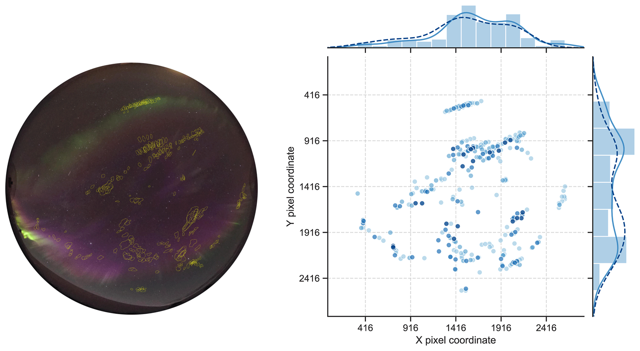
Figure 1 All 262 identified FAE candidates for event 3 on 18 December 2017 (left panel), overlain on the first image of the series taken at 07:36:35 UTC. The FAE candidates occurred over a time period of ∼ 50 min. Geomagnetic east corresponds to the left-hand side of the image and geomagnetic north to the top. All 305 FAE locations (right panel) are then plotted in horizontal and vertical pixel coordinates, with the corresponding histogram distribution and kernel density estimation (KDE). FAEs are shaded according to confidence groups, with darker shades being FAEs of a higher quality. The dashed KDE line is only calculated for FAEs of groups 1 and 2. Credit: all-sky camera (ASC) image provided by the KHO.

Visual inspection of all events shows that FAEs appear mostly elliptical; thus, fitting an ellipse to follow the marked outline of each FAE provides a more robust estimate of its size. As shown in Fig. 2, the fitted ellipses of most FAEs have a major axis of 20 km or less, with a few larger outliers that might simply be diffuse auroral patches, especially on the larger end of the marked size range. The average major axis length is ∼ 6–8 km, with an average minor axis of ∼ 3–4 km. Their aspect ratio (AR $=\left[\text{Major axis}\right]/\left[\text{Minor axis}\right]$) has a mean value of 2.04. Most FAEs seem to have fairly regular, rounded shapes with few indents, with a mean circularity value of c=0.705 (c=1 being perfectly circular), which is determined using the formula $c=\mathrm{4}\mathit{\pi }\cdot \left[\text{Area}\right]/[\text{Perimeter}{]}^{\mathrm{2}}$. This determination is, of course, affected by their size, with deviations from rounded shapes being harder to identify in smaller FAEs, with an added general operator bias to outline regular shapes compared to complex indents. It should be noted that, due to the 4 s integration time of the ASC, any fast-moving object will appear somewhat elliptical. Nevertheless, this is not true for the high-frame-rate data from ASK, which also show FAEs to be elliptical. The described trends are observable in both high- and low-quality candidates, as KDEs for high-quality FAEs are in good agreement with the entire data set in Fig. 2. This suggests that most of the marked candidates of groups 3 and 4 are indeed FAEs.

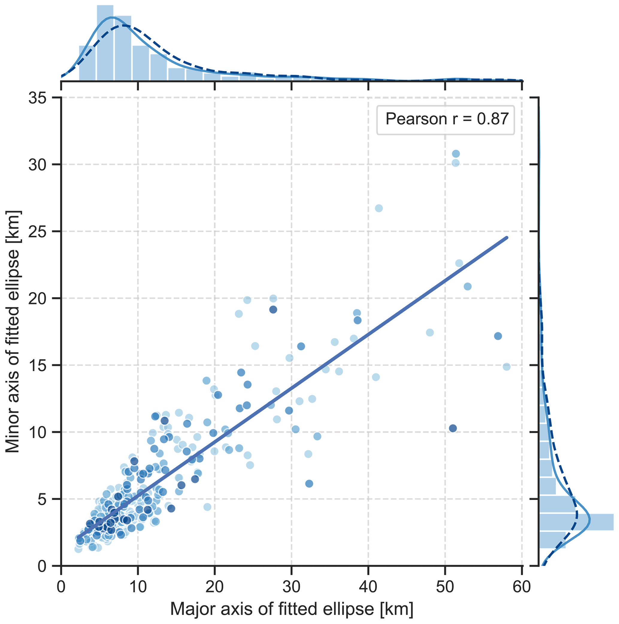
Figure 2 Length of major and minor axes (in kilometres) of fitted ellipses for each FAE, assuming an altitude of 110 km. FAEs are shaded according to confidence groups, with darker shades being FAEs of higher quality. A histogram of the variables is plotted on the outer axes, together with a KDE. The dashed KDE line is only calculated for FAEs of groups 1 and 2. The legend shows the calculated statistical Pearson correlation coefficient for a linear regression, with a p value ≪ 0.01, which rejects the null hypothesis.

Category 2 FAEs can be seen moving along the auroral arc in Fig. 3. The distance between these FAEs does not vary significantly as they move eastward over a period of 35 s. A spatial intensity variation is visible in the grouped structure, where FAEs appear dim towards the edges of the group and become more intense the closer they move towards the centre. Some of the variation in intensity seems to be caused by fragments appearing and disappearing at the ends of the group. Using an average distance of 45 pixels between the FAEs and their approximate elevation angle of ∼ 65^∘, we can roughly estimate the spacing between FAEs for this group to be around ∼ 6 km.

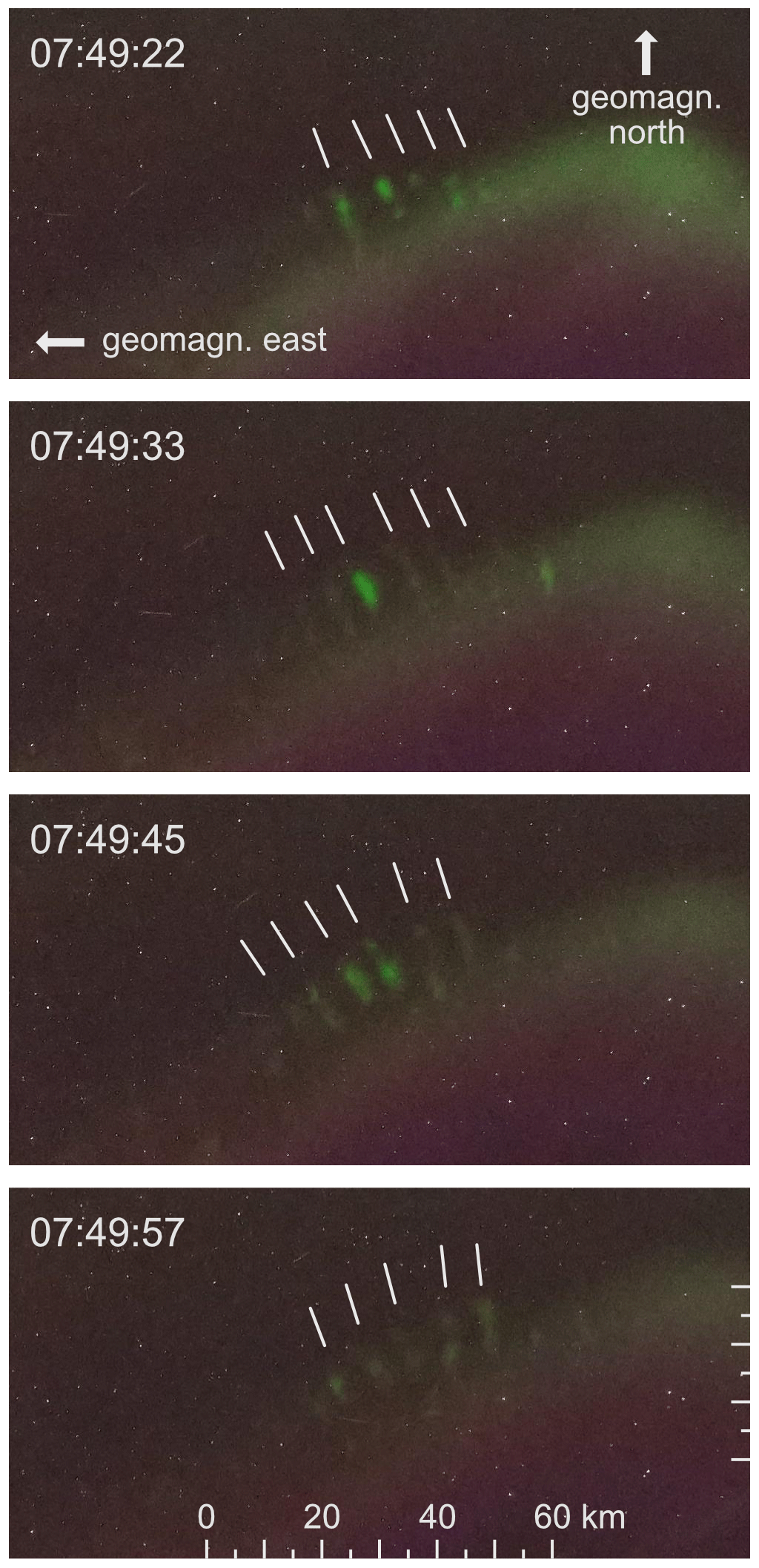
Figure 3 Movement of a category 2 FAE group northwards of the main auroral arc (northwest of zenith) over four successive images taken on 18 December 2017 around 07:49:40 UTC. The images are cropped to 1000 × 500 pixels to make the FAEs easily identifiable. White lines indicate the apparent alignment of the FAEs and were used to determine approximate distances between them. A scale (in kilometres) is added for reference, using a pixel to kilometre ratio of 0.129 (at 65^∘ elevation angle). Credit: ASC images provided by the KHO.

Visual inspection of the ASC images shows a general westward movement of the FAEs for the observed events, which might originate from the underlying convection pattern. No obvious eastward motion was observed. A few FAEs were observed in the ASK high-frame-rate images (see Fig. 5), with some remaining stable for multiple seconds while they drift, whereas others appeared and vanished within a second. The ASK FOV corresponds to 10 × 10 km² at an altitude of 100 km, which FAEs passed within ∼ 10–14 s. This results in an estimated drift speed of the order of ∼ 1 km s⁻¹.

3.2 Observed emissions

For FAE positioned along the MSP scanning line, the MSP data were checked to search for corresponding signatures. Three FAE signatures were found, of which one is presented in Fig. 4. Distinct FAE emissions were observed at the 557.7 nm (green MSP channel) line of atomic oxygen but not at the 630.0 nm (red channel) line of atomic oxygen nor at the 427.8 nm (blue channel) emission of ${\mathrm{N}}_{\mathrm{2}}^{+}$. Due to the long lifetime of the 630.0 nm emission state (∼ 110 s) and the short-lived and fast-moving nature of FAEs, the respective MSP red channel measurements are unlikely to show any distinct FAE signatures, with any potential emissions being smeared over the temporal axis.

Figure 4 Comparison of consecutive cropped ASC images and MSP line scans for a FAE moving through the MSP scan line on 18 December 2017 between 07:48:23–47 UTC. The FAE signatures are marked with vertical lines in the green channel (557.7 nm). The MSP scan line (1^∘ width) is drawn on the ASC images in grey. A grey square marks the geographic zenith in the centre of the ASC images. Credit: ASC images provided by the KHO.

Figure 4 shows a clear peak at the FAE elevation of ∼ 100^∘ in the 557.7 nm measurements while it passed the MSP scan line (marked by vertical lines), with a clear drop-off as the FAE moved out of the scan and faded. No distinct signature can be seen at this elevation in the 427.8 nm measurements. A broad general increase is visible over a large area in the 630.0 nm emissions, likely caused by the background aurora at higher altitudes, as this emission was elevated before and after the FAE occurrence. Also, at the suggested FAE altitude of ∼ 110 km, the atomic oxygen state which emits at 630.0 nm is heavily collisionally quenched, and thus, any FAE emissions at this wavelength at low altitudes are expected to be extremely weak. It should, nonetheless, be noted that the broad increase may potentially hide a FAE signature in the 630.0 nm data. The other MSP passings show comparable results.

One FAE was observed passing through the ASK FOV during event 2 on 7 December 2015 (for the corresponding video file, see Whiter, 2020). The ASK instrument provides temporal and spatial high-resolution observations. N₂ emission signatures at 673.0 nm (first positive band system) in the ASK channel 1 data can be seen in Fig. 5b and c. At the same time, no emission is visible in Fig. 5d, which shows the ASK channel 3 measurement at 777.4 nm (atomic oxygen). The ratio between $\mathrm{777.4}/\mathrm{673.0}$ nm emissions is commonly used to determine the energy of precipitating particles, and typically, the lack of 777.4 nm emissions resulting in very small ratios would mean high energy precipitation (e.g. Lanchester et al., 2009; Dahlgren et al., 2016). But, even with very high energies, there should be some 777.4 and 427.8 nm emissions. The apparent lack of these emissions suggests a different generation mechanism to precipitation. As the FAEs show emissions at 557.7 and 673.0 nm, but seemingly not at 427.8 or 777.4 nm, looking at the excitation thresholds of these emissions can give a clue regarding the upper energy limits of the generation mechanism. Excitation thresholds for the 427.8 and 777.4 nm emissions lie above 10 eV (e.g. Lanchester et al., 2009; Holma et al., 2006), with the lowest possible excitation energy being ∼ 11 eV for the direct excitation of atomic oxygen at 777.4 nm. For the observed 557.7 and 673.0 nm emissions, the excitation energies are 2 and ∼ 8 eV, respectively (e.g. Holma et al., 2006; Ashrafi et al., 2009). Combined, this suggests an upper limit for the energy of the generation mechanism between ∼ 8–11 eV.

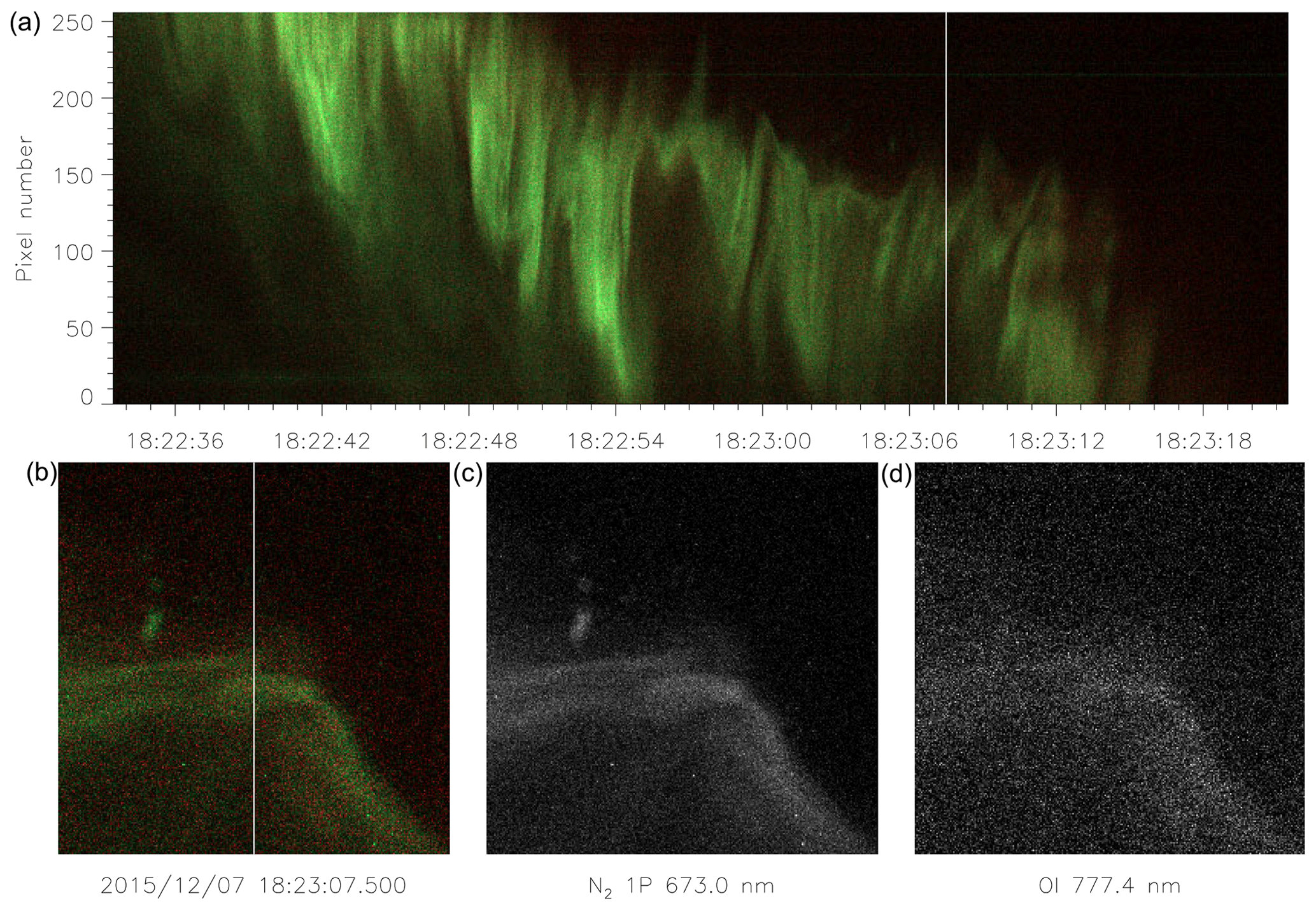
Figure 5 ASK keogram for the event of 7 December 2015 around 18:23:07 UTC in panel (a). ASK1 measuring the 673.0 nm emission of the first positive band system of N₂ is visible in (c), (d) shows the ASK3 measurement of 777.4 nm emissions of atomic oxygen, and (b) shows ASK1 in the green/blue channel and ASK3 in the red channel.

3.3 Plasma characteristics measured with the ESR

To further understand the underlying plasma properties of FAEs, an attempt was made to find signatures within incoherent scatter data of the ESR. The auroral arc visible south of the FAE in Fig. 5 extended across the entire FOV of ASK (partially shared with the ESR) shortly before the FAE occurrence at 18:23 UTC and is visible in Fig. 6 as a general increase in electron density across the entire altitude range. The density decreases across most altitudes as the arc moves out of the FOV towards 18:23 UTC. It remains high at 113 km at the time of the FAE occurrence. No associated increase in electron temperatures is visible in Fig. 6 for the period and altitudes of the arc signature in the electron density panel.

The FAE visible in Fig. 6 shows as a local increase in electron temperature to ∼ 2300 K at 113 km around 18:23 UTC. This increase seems to be confined to a narrow altitude range, which is further established by the time series at four successive altitudes shown in Fig. 7. The increase at the time of the FAE passing is limited to altitudes below 119 km and is strongest at 113 km. For the period directly after the FAE occurrence, multiple increases in electron temperature are visible at low altitudes, which indicates an unstable lower ionosphere. Simultaneous increases in ion temperatures are visible at higher altitudes, with significant increases around 190 km, up to ∼ 4500 K.

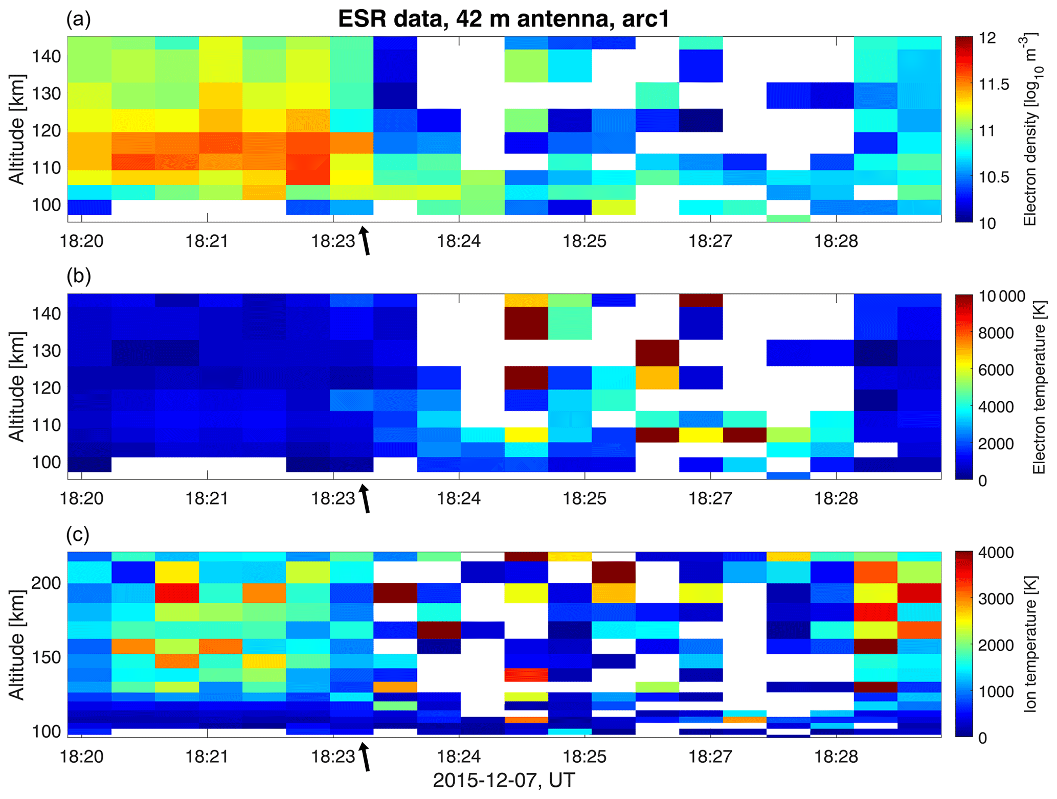
Figure 6 Incoherent scatter data from the ESR (analysed with GUISDAP (Grand Unified Incoherent Scatter Design and Analysis Package) software) for 18:20–18:30 UTC on 7 December 2015, with electron densities in (a), electron temperatures in (b), and ion temperatures in (c). Data points with errors > 50 % of the values were removed. Further limiting to > 30 % would only remove a few extra data points. Errors for the relevant time periods up to the FAE passing are < 20 % of the values. The arrows mark the time of the FAE passing.

Figure 7 Time series of electron temperatures at four successive altitudes between 105–119 km from incoherent scatter data from the ESR (analysed with GUISDAP) for 18:20–18:26 UTC on 7 December 2015. Data points with errors > 50 % of the values were removed. The arrow marks the time of the FAE passing and denotes the distinct increase in electron temperature specifically at 113 km.

The background conditions during these analysed events might be able to further provide some insight into the underlying generation mechanism. For the entire duration of event 3, significant intermittent increases in electron temperatures were observed at altitudes in the E region and elevated ion temperatures (mostly) in the F region. This indicates a connection between FAEs and elevated electron temperatures at low altitudes, which we will discuss below.

4 Discussion

Fragmented aurora-like emissions (FAEs) have been analysed and classified in the present study, with results suggesting that they are a new type of aurora-like feature. Comparing FAEs with ostensibly similar auroral phenomena shows some key differences. For example, the term enhanced aurora (EA; see Hallinan et al., 1985) describes an enhanced emission in a thin layer, typically along a rayed auroral structure. Although it also designates a localised emission intensity enhancement occurring alongside aurorae, EA differs in various characteristics. EA occurs as layers with limited vertical extent but has longitudinal and latitudinal extents of at least 250 and 300 km, respectively (Hallinan et al., 1985). FAEs are much smaller, with minor and major axes sizes of < 10 km. While EA manifests as intensity enhancements along the rays of a bigger auroral feature, FAEs were clearly dislocated from the field lines of the adjacent rayed structures. FAEs also lack the blue emission enhancement visible in EA. Furthermore, EA has been observed as quasi-stable structures lasting for minutes, while most analysed FAEs had lifetimes of less than a minute. Overall, this suggests that these are two different phenomena.

When comparing FAEs with pulsating patches, two major distinctions between the two phenomena are size and lifetime of the individual features. Pulsating patches occur within diffuse aurorae, whereas the analysed FAEs are seen alongside discrete arcs. FAEs are much smaller than pulsating patches, which are also typically very stable, while showing quasi-periodic fluctuations in their emission intensity (e.g. Humberset et al., 2018; Nishimura et al., 2020). In contrast, FAEs are short-lived and do not show any emission intensity fluctuations, apart from appearing and fading away. The available ASK video observations of FAEs show their much higher dynamic motion and smaller size, compared to pulsating patches. Together, these differences lead us to conclude that FAEs are a distinctly different phenomenon.

As the FAEs were found by a manual inspection of images, there is some bias in terms of which features were selected and how they were classified. The data set could contain other auroral small-scale forms or diffuse patches, which is the reason for the classification into four confidence groups. As the general properties of candidates between high- and low-confidence groups agree well, we are confident that most selected features are indeed FAEs. Generally, FAEs can be distinguished from other auroral forms by their lack of field-aligned emission extent, as suggested by the off-zenith parts of the ASC images and field-aligned ionisation measured by the ESR, small sizes and short lifetimes. A FAE signature is visible in the ESR data as locally enhanced electron temperatures around 113 km. Determining a definite FAE altitude requires triangulation, which was not possible for the analysed ASC images or other means of consistently identifying FAE signatures in measurements over an altitude range, such as multiple signatures in EISCAT data.

Semeter et al. (2020) recently described green streaks below STEVE, which show various similarities to FAEs. Their triangulation positions the streaks at an altitude of 100–110 km, which is also the region within which we suggest FAEs occur. They propose superthermal electrons resulting from the extreme electric fields during STEVE as a local generation mechanism, similar to our hypothesis. It will be interesting to see if these two phenomena are indeed related on a fundamental level or just bear superficial resemblance. Gallardo-Lacourt et al. (2018) suggest STEVE as another locally generated skyglow without any associated particle precipitation. The phenomenon is far from well understood and occurs on much larger scales than FAEs but indicates that ionospheric processes can indeed cause emission without particle precipitation being present. We propose that FAEs fall within the same category, even though many of their properties, such as size and lifetime, differ majorly. The underlying processes heating the plasma are unlikely to be the same, but on a fundamental level, both emissions seem to be related to thermal ionospheric processes rather than particle precipitation.

The present study aims to present the basic characteristics of FAEs and categorise them based on the three analysed events. Nonetheless, the available data enable us to hypothesise about their underlying generation mechanism. The analysed events show above-average solar wind speeds (except for event 1), negative IMF B_z, and positive B_y, with a westward convection of FAEs. They are not limited to a certain time sector, with occurrences both between 10:30–11:30 and 21:15–23:15 magnetic local time (MLT). The elevated electron temperature at E-region altitudes and simultaneous increases in ion temperatures at higher altitudes can provide some clues about the origin of FAEs. One possible group of generation mechanisms for the required energy to excite FAEs are Farley–Buneman instabilities, which are streaming instabilities typically occurring at altitudes of 90–120 km (Oppenheim et al., 1996). The proposed FAE altitude falls within this region. They become significant when the difference between electron and ion drift speeds exceeds the ion acoustic speed (Liu et al., 2016), which is generally the case in geomagnetically disturbed conditions, typically also resulting in aurorae. This would explain why FAEs are observed alongside aurorae. Particularly at high latitudes, these instabilities can result in significant local electron heating. This is consistent with the low-altitude elevated electron temperatures observed during the FAE events, for which Farley–Buneman instabilities are the most likely explanation.

The observed large ion temperatures in the F region around 190 km height are caused by Joule heating from strong electric fields or ion-neutral friction. The measurements are used to estimate the electric field strength below, assuming that $E_{\parallel }=\mathrm{0}$, i.e. the magnetic field lines, are equipotentials. We neglect the effect of the slightly different magnetic field strengths between 190 km height and the lower E region, and also any differences in the neutral wind between these altitudes. The ion energy balance, neglecting also thermal energy transfer to/from electrons (whose temperatures are generally not enhanced above the E region, especially preceding the FAE occurrence at 18:23 UTC) is (Alcayde et al., 1983, Eq. 4):

$$\begin{array}{}\text{(1)}& Q_{\mathrm{in}}={\mathit{\nu }}_{\mathrm{in}}{N}_{\mathrm{n}}{N}_{\mathrm{e}}\left({\displaystyle \frac{\mathrm{3}}{\mathrm{2}}}{k}_{\mathrm{B}}\left(T_{\mathrm{n}}-T_{\mathrm{i}}\right)+{\displaystyle \frac{\mathrm{1}}{\mathrm{2}}}{m}_{\mathrm{i}}{\left({\mathit{V}}_{\mathrm{i}}-{\mathit{V}}_{\mathrm{n}}\right)}^{\mathrm{2}}\right)\end{array}$$

Here, T_i and T_n are the ion and neutral temperatures, and V_i and V_n are the ion and neutral drifts, respectively. m_i is the mean ion mass, k_B is the Boltzmann constant, ν_in is the ion-neutral collision frequency, and N_n and N_e are the neutral and electron densities. In the steady-state Q_in=0, and for the F region, we insert $\left({\mathit{V}}_{\mathrm{i}}-{\mathit{V}}_{\mathrm{n}}\right)={\mathit{E}}_{⟂}\times \mathit{B}/B^{\mathrm{2}}$ with E_⟂ the electric field in the frame of the neutral gas and B the geomagnetic field. We are only interested in the magnitude of E_⟂, which can be estimated as follows:

$$\begin{array}{}\text{(2)}& E_{⟂}/B=\sqrt{\mathrm{3}{k}_{\mathrm{B}}\left(T_{\mathrm{i}}-T_{\mathrm{n}}\right)/m_{\mathrm{i}}}.\end{array}$$

Filtering out elevated ion temperatures above 1500 K, we use the ESR data to estimate a mean background ion temperature in the quiet state of ∼ 950 K for the altitude range of 150–300 km, which should then approximately correspond to the neutral temperature. For m_i, we conservatively use 30 amu, corresponding to a mixture between ${\mathrm{N}}_{\mathrm{2}}^{+}$ and ${\mathrm{O}}_{\mathrm{2}}^{+}$, neglecting a contribution by O⁺. The motivation is that high T_i and large drift difference |V_i−V_n| probably enhance the relative molecular concentration compared to model values, as the International Reference Ionosphere (IRI) would give it. Using average elevated T_i≈ 3300 K for the altitude range of 150–300 km from the ESR measurement, the estimated lower limit is $E_{⟂}\approx$ 70 mV m⁻¹. This value is far above the threshold for Farley–Buneman instabilities, which is typically around 30 mV m⁻¹ (Williams et al., 1992). If molecular ions were assumed to be dominant, it would only further increase the lower limit. It should be noted that this is an approximation, and the filtering for average values is based on somewhat arbitrary choices, but the derived E_⟂ is not all that dependent on the inserted T_i and T_n and would exceed the typical limit for Farley–Buneman instabilities by a significant margin regardless of the exact filtering values. The threshold may already be exceeded in the arc, before 18:23 UTC, but T_e was perhaps not high enough to excite optical emissions. Buchert et al. (2008) showed an example with the ESR, where T_e reaches temperatures above 3000 K at 100–109 km, which is enough to produce 630.0 nm optical emissions, according to Gustavsson et al. (2001). An open question is whether these instabilities can produce large enough T_e increases to excite all observed FAE emissions. Buchert et al. (2008) showed that T_i increased already above ∼ 125 km, up to about 4000 km. These temperature enhancements are stronger than those observed at auroral oval latitudes over mainland Norway by Williams et al. (1992). This could be because, at the edge of the auroral oval over Svalbard, E fields may be larger than in the auroral zone, or because the ESR is more sensitive than the EISCAT mainland radar was in 1992. If E fields (and associated T_e enhancements) are typically larger at Svalbard, this might perhaps explain why FAEs have not been noticed earlier in the auroral zone or along the Scandinavian mainland. Another possible contributing factor could be that auroral all-sky cameras used for scientific purposes are often more limited in pixel resolution compared to the Sony α7S used in the present study, which could reduce the likelihood of unexpectedly identifying small-scale and short-lived features like FAEs.

Whereas specific characteristics for the individually occurring FAEs are hard to identify, category 2 FAE groups with regular spacing clearly suggest a link to wave activity. We tentatively suggest that waves modulate the electric field strength and correspondingly the intensity of Farley–Buneman-induced plasma turbulence and electron heating near the arcs to produce the observed category 2 FAE groups. As these groups show regular and fairly stable distances between the individual FAEs, some kind of monochromatic wave seems to be responsible. Suzuki et al. (2009) describe the modulation of airglow by gravity waves, which is similar to the modulation of category 2 FAE groups, albeit at larger scales. The short distances between FAEs suggests waves with small wavelengths. The estimated FAE drift speed of ∼ 1 km s⁻¹ is much faster than the average ionospheric convection speed of a few hundred metres per second. If category 2 FAEs are indeed modulated by waves, they could propagate with their phase velocity and thus exceed typical convection speeds. Alternatively, the E-field modulation could originate from the magnetosphere. A candidate mechanism is that the shear between the strong flow in the high E field adjacent to the arc and the slower flow in the arc itself leads to a Kelvin–Helmholz instability, whose phase speed would be between the slow and fast flows (see, e.g., Keskinen et al., 1988). For $E_{⟂}\approx$ 70 mV m⁻¹ corresponding to 1400 m s⁻¹, the phase speed of Kelvin–Helmholtz waves would be several hundred metres per second, which is roughly the observed value. It is, however, unclear why the auroral arc shows no signature of the modulation and what determines the wavelength of the quasi-periodic FAEs of ∼ 6 km.

To determine a link between FAEs and other aurora-like features like STEVE or the green streaks, and to further analyse FAE characteristics, more events will need to be studied, ideally from multiple locations and with ionospheric plasma measurements. The limited sample size, not necessarily of FAEs, but rather observation nights and ESR data for the present study, limits the conclusions that can be drawn for the underlying generation mechanism. Until these conditions are determined, FAE occurrences will be seemingly random, further complicating a targeted follow-up study.

5 Conclusions

The focus of the present study is to characterise a new type of aurora-like phenomenon, which we name fragmented aurora-like emissions (FAEs). In summary, the observed FAEs can be grouped into two categories, namely individually occurring FAEs and groups close to auroral arcs with a wave-like structure. All FAEs show a lack of field-aligned extent and seem to generally occur in the shape of an elongated ellipse. The majority of the observed FAEs have a major axis smaller than 20 km (assuming an altitude of ∼ 110 km), with a mean aspect ratio of ∼ 2. Photometer data show distinctly enhanced intensities at the 557.7 nm emission of atomic oxygen for FAEs passing the FOV but no clear FAE signatures at the 427.8 and 630.0 nm wavelengths, of which the latter is not surprising as it would be heavily collisionally quenched at the proposed altitude. A FAE signature is also clearly visible in the ASK1 673.0 nm emission channel of the first positive band system of N₂ but not at the 777.4 nm emission of atomic oxygen measured by ASK3, which together sets a range of states with different energies that are excitable by the generation mechanism. The apparent lack of 427.8 and 777.4 nm emissions indicates an upper energy limit between ∼ 8–11 eV which the generation mechanism can produce. The ESR data suggest that FAEs are associated with significantly elevated electron temperatures around 110–120 km, for which Farley–Buneman instabilities are the only known cause at these low altitudes. Simultaneously, increased ion temperatures are visible at altitudes in the F region, which enables us to estimate the strength of the E field. The derived estimate of $E_{⟂}\approx$ 70 mV m⁻¹ exceeds the typical Farley–Buneman threshold of 30 mV m⁻¹. Category 2 FAE groups show a fairly regular and stable spacing and appear to be modulated by some kind of wave.

Open questions are the exact nature of the generation mechanism, such as whether FAEs of categories 1 and 2 are caused by the same mechanism, if category 2 FAEs are indeed modulated by wave activity, and, if so, by what kind of wave, whether they are exclusively a high-latitude phenomenon, and what threshold values of ionospheric parameters are necessary for FAE occurrences.