Semi-annual variation of excited hydroxyl emission at mid-latitudes

Ground-based observations show a phase shift in semi-annual variation of excited hydroxyl (OH^∗) emissions at mid-latitudes (43^∘ N) compared to those at low latitudes. This differs from the annual cycle at high latitudes. We examine this behaviour by utilising an OH^∗ airglow model which was incorporated into a 3D chemistry–transport model (CTM). Through this modelling, we study the morphology of the excited hydroxyl emission layer at mid-latitudes (30–50^∘ N), and we assess the impact of the main drivers of its semi-annual variation: temperature, atomic oxygen, and air density. We found that this shift in the semi-annual cycle is determined mainly by the superposition of annual variations of temperature and atomic oxygen concentration. Hence, the winter peak for emission is determined exclusively by atomic oxygen concentration, whereas the summer peak is the superposition of all impacts, with temperature taking a leading role.

1 Introduction

Since the second half of the 20th century, emissions of excited hydroxyl have been used for three main purposes: (1) to infer information about temperature and its long-term change; (2) to obtain distributions of minor chemical constituents (O₃, H, and O) at the altitudes of the mesopause; and (3) to investigate dynamic processes such as tides, gravity, and planetary waves (GWs and PWs, respectively); sudden stratospheric warmings (SSWs); and the quasi-biennial oscillation (QBO).

Hence, a number of authors have studied temperatures in the mesopause region using airglow emission ground-based observations focusing on long-term trends (e.g. Bittner et al., 2002; Holmen et al., 2014; Dalin et al., 2020, and references therein) with attention to seasonal variations (e.g. Reid et al., 2017, and references therein) and the solar-cycle effect (e.g. Kalicinsky et al., 2016, and references therein).

Minor chemical constituents as well as chemical heat have also been retrieved by OH^∗ emission observations. Ever since atomic oxygen concentration was determined by the rocket-borne detection of OH^∗ airglow (Good, 1976), this method has come into wide use for obtaining information about distributions of minor chemical constituents in the mesopause region, namely, atomic oxygen concentration (e.g. Russell et al., 2005; Mlynczak et al., 2013a, and references therein), ozone concentration (e.g. Smith et al., 2009, and references therein), atomic hydrogen concentration (e.g. Mlynczak et al., 2014, and references therein), and exothermic chemical heat (e.g. Mlynczak et al., 2013b, and references therein). In future, excited hydroxyl airglow could be used for measurements of hydroperoxy radicals and water vapour concentrations (Kulikov et al., 2009, 2018b; Belikovich et al., 2018b).

Numerous studies using airglow observations, have been devoted to dynamic processes, e.g. to study mesopause variabilities in time of SSWs (Damiani et al., 2010; Shepherd et al., 2010). Gao et al. (2011) studied the temporal evolution of nightglow brightness and height during SSW events. A year earlier, they found a QBO signal in the excited hydroxyl emission (Gao et al., 2010). The climatology of PWs was investigated in studies by Takahashi et al. (1999), Buriti et al. (2005), and Reisin et al. (2014). Tides were studied by Xu et al. (2010) and Lopez-Gonzalez et al. (2005). GW parameters based on the airglow technique were investigated, e.g. by Taylor et al. (1991) and Wachter et al. (2015). A more complete description of studies in which hydroxyl emissions were used to study dynamic processes can be found in a review by Shepherd et al. (2012).

The morphology of the OH^∗ layer is an essential component in the interpretation of observations and in understanding the processes involved in layer variability. Annual variations in the OH^∗ layer have been identified at all latitudes (Marsh et al., 2006). Equatorial and low-latitude semi-annual variations have been observed by satellites (e.g. Abreu and Yee, 1989; Liu et al., 2008, and references therein), as well as by ground-based instruments (Takahashi et al., 1995), and they have been modelled by several research teams (Le Texier et al., 1987; Marsh et al., 2006, and references therein). The maxima of emissions were found to occur near equinoxes. In spite of the large number of studies on this subject, there are still knowledge gaps. Recently, unexpected behaviour in the semi-annual cycle of excited hydroxyl emission has been found by ground-based observations, with a shift of the peaks from equinoxes to summer and winter at middle latitudes (Popov et al., 2018, 2020); this was also found by modelling (Grygalashvyly et al., 2014; Fig. 3). Similar variations in OH^∗ emissions with peaks near equinoxes have been observed at middle latitudes (34.6^∘ N) in the Southern Hemisphere (Reid et al., 2014). These results were provided without explanations; in our short paper, we offer a preliminary explanation.

The second section of our article describes the observational technique and model that were applied; in the third section, we present results and an analysis of observations and modelling; conclusions are provided in the fourth section.

2 Observational technique and model

2.1 Observational technique

The spectral airglow temperature imager (SATI), which measures nightglow intensity for vibrational transitions of ${\mathrm{OH}}_{\mathit{\text{v}}=\mathrm{6}}^{\ast }$ → ${\mathrm{OH}}_{\mathit{\text{v}}=\mathrm{2}}^{\ast }$ and temperature using vibrational-rotational transitions, was assembled at the Institute of Ionosphere (43^∘ N, 77^∘ E) in Almaty, Kazakhstan. It represents a Fabry–Perot spectrometer with a CCD (charge-coupled device) camera as a detector and a narrowband interference filter as the etalon. Following Lopez-Gonzalez et al. (2007), we use an interference filter with the centre at 836.813 nm and a bandwidth of 0.182 nm. This corresponds to the spectral region of the ${\mathrm{OH}}_{\mathit{\text{v}}=\mathrm{6}}^{\ast }$ → ${\mathrm{OH}}_{\mathit{\text{v}}=\mathrm{2}}^{\ast }$ band. In order to infer the temperature, the calculated spectra for different vibro-rotational transitions are compared with those from observations. The SATI operates at a 60 s exposure that provides corresponding time resolution. The method of temperature retrieval is well-described by Lopez-Gonzalez et al. (2004). The observations of temperature were validated using satellite SABER measurements (Lopez-Gonzalez et al., 2007; Pertsev et al., 2013). Additional details about this instrument are presented in many papers (Wies et al., 1997; Aushev et al., 2000; Lopez-Gonzalez et al., 2004, 2005, 2007, 2009). The analysis presented in this paper uses data averaged over the years 2010–2017.

2.2 Model and numerical experiment

The model of excited hydroxyl (MEH) calculates the OH^∗ number densities at each vibrational level v as the production divided by losses (excited hydroxyl is assumed in the photochemical equilibrium), which include the chemical sources as well as collisional and emissive removal:

$$\begin{array}{}\text{(1)}& \left[{\mathrm{OH}}_v\right]={\displaystyle \frac{\left(\begin{array}{l}{\mathit{\varsigma }}_v{a}_{\mathrm{1}}\left[{\mathrm{O}}_{\mathrm{3}}\right]\left[\mathrm{H}\right]\\ +{\mathit{\psi }}_v{a}_{\mathrm{2}}\left[\mathrm{O}\right]\left[{\mathrm{HO}}_{\mathrm{2}}\right]\\ +{\sum }_{v^{\prime }=v+\mathrm{1}}^{\mathrm{9}}{B}_{v^{\prime }v}\left[{\mathrm{O}}_{\mathrm{2}}\right]\left[{\mathrm{OH}}_{v^{\prime }}\right]\\ +C_{v+\mathrm{1}}\left[{\mathrm{N}}_{\mathrm{2}}\right]\left[{\mathrm{OH}}_{v+\mathrm{1}}\right]\\ +{\sum }_{v^{\prime }=v+\mathrm{1}}^{\mathrm{9}}{D}_{v^{\prime }v}\left[\mathrm{O}\right]\left[{\mathrm{OH}}_{v^{\prime }}\right]\\ +{\sum }_{v^{\prime }=v+\mathrm{1}}^{\mathrm{9}}{E}_{v^{\prime }v}\left[{\mathrm{OH}}_{v^{\prime }}\right]\end{array}\right)}{\left(\begin{array}{l}{a}_{\mathrm{3}}\left(v\right)\left[\mathrm{O}\right]+{\sum }_{v^{\prime \prime }=\mathrm{0}}^{v-\mathrm{1}}{D}_{v{v}^{\prime \prime }}\left[\mathrm{O}\right]\\ +C_v\left[{\mathrm{N}}_{\mathrm{2}}\right]\\ +{\sum }_{v^{\prime \prime }=\mathrm{0}}^{v-\mathrm{1}}{B}_{v{v}^{\prime \prime }}\left[{\mathrm{O}}_{\mathrm{2}}\right]\\ +{\sum }_{v^{\prime \prime }=\mathrm{0}}^{v-\mathrm{1}}{E}_{v{v}^{\prime \prime }}\end{array}\right)}},\left(\begin{array}{c}v<v^{\prime }\\ v^{\prime \prime }<v\end{array}\right).\end{array}$$

Table 1 List of reactions with corresponding reaction rates (for three-body reactions [${\mathrm{cm}}^{\mathrm{6}}{\mathrm{molecule}}^{-\mathrm{2}}{\mathrm{s}}^{-\mathrm{1}}$] and for two-body reactions [${\mathrm{cm}}^{\mathrm{3}}{\mathrm{molecule}}^{-\mathrm{1}}{\mathrm{s}}^{-\mathrm{1}}$]), branching ratios, quenching coefficients, and spontaneous emission coefficients (s⁻¹) used in the paper.

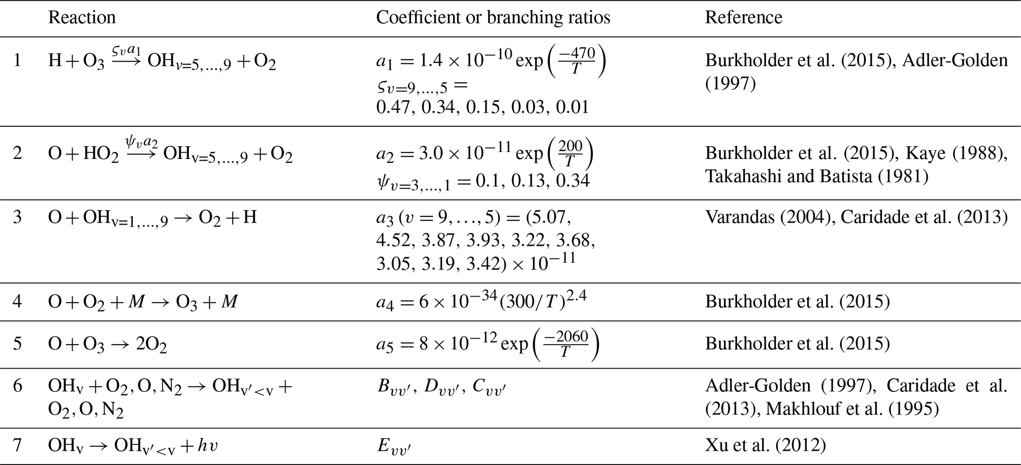
The first term in the numerator of Eq. (1) is the reaction ${\mathrm{O}}_{\mathrm{3}}+\mathrm{H}\to {\mathrm{OH}}_{\mathit{\text{v}}}+\mathrm{O}$, where a₁ is the reaction rate, and ς_v represents the branching ratios (Adler-Golden, 1997). The second term is the $\mathrm{O}+{\mathrm{HO}}_{\mathrm{2}}\to {\mathrm{OH}}_{\mathit{\text{v}}}+{\mathrm{O}}_{\mathrm{2}}$ reaction, where a₂ and ψ_v are the reaction rate and nascent distribution, respectively (Kaye, 1988, after Takahashi and Batista, 1981). The other three summands represent the populations resulting from collisional relaxation from higher v levels, where B, C, and D are the collisional deactivation coefficients for O₂ (Adler-Golden, 1997), N₂ (Makhlouf et al., 1995), and O (Caridade et al., 2013), respectively. The last summand is the multi-quantum population by spontaneous emissions, where $E_{v^{\prime }v}$ is the spontaneous emission coefficient (Xu et al., 2012). The losses occur, additionally, through the chemical removal of the excited hydroxyl by atomic oxygen, where a₃(v) is the vibrationally dependent reaction rate (Varandas, 2004). The calculations in Eq. (1) are incorporated into the chemistry–transport model (CTM). We calculate volume emission for transition ${\mathrm{OH}}_{\mathit{\text{v}}=\mathrm{6}}^{\ast }$ → ${\mathrm{OH}}_{\mathit{\text{v}}=\mathrm{2}}^{\ast }$ as the product of the Einstein coefficient for given transition by concentration of excited hydroxyl at corresponding vibrational number, i.e. $V_{\mathrm{62}}=E_{\mathrm{62}}\left[{\mathrm{OH}}_{\mathrm{6}}^{\ast }\right]$. All reactions used in Eq. (1) and in the appendix – together with corresponding reaction rates, branching ratios, quenching rates, and spontaneous emission coefficients, besides those for multi-quantum processes – are collected in Table 1.

Here, we enumerate only the main features of the CTM as one can find extended descriptions in many studies (Sonnemann and Grygalashvyly, 2020; Grygalashvyly et al., 2014; and references therein). The CTM consists of four blocks: chemical, transport, radiative, and diffusive. The chemical block accounts for 19 constituents and 63 photodissociations and chemical reactions (Burkholder et al., 2015). The chemical code utilises a family approach with the odd oxygen (O(¹D), O, O₃), odd hydrogen (H, OH, HO₂, H₂O₂), and odd nitrogen (N(²D), N(⁴S), NO, NO₂) families (Shimazaki, 1985). In the radiative part, the dissociation rates are taken from a precalculated table depending on zenith angle and altitude (Kremp et al., 1999). The transport block calculates advection in three directions following Walcek (2000). The diffusive part accounts for only vertical molecular plus turbulent diffusion (Morton and Mayers, 1994). This model has been validated against observations of ozone, which plays a role in the formation of OH^∗ (e.g. Hartogh et al., 2011; Sonnemann et al., 2007; and references therein) and water vapour, which is the principal source of odd hydrogens and, particularly, of atomic hydrogen (e.g. Hartogh et al., 2010; Sonnemann et al., 2008; and references therein). Our current analysis used the run for year 2009 (the choice of this year does not affect our conclusions, because calculations for other years show similar semi-annual variations), which was published and described in a number of studies (Grygalashvyly et al., 2014, Sect. 4; Sonnemann et al., 2015). This run is based on the dynamics and temperature of the LIMA (Leibniz Institute Middle Atmosphere) model for the so-called “realistic case”, in which carbon dioxide, ozone, and Lyman-α flux are taken from observations, and the horizontal winds and temperature of ECMWF (European Centre for Medium-Range Weather Forecasts) are assimilated below ∼ 35 km (Berger, 2008; Lübken et al., 2009, 2013).

Here we assume that the structures in the longitudinal direction are equivalent to local time (LT) behaviour, with 24:00 LT related to midnight at 0^∘ longitude. The local times of successive longitudes are used to analyse our calculations. Hence, in the following figures related to the model results, longitude is used as the so-called “pseudo time”. The night-time averaged values account for the period from 21:45 to 02:15 LT. For the purposes of our discussion, we use “pressure-altitude” (or in other words “pseudo-altitude”) $Z^{\ast }=-H\ln (P/P_{\mathrm{0}})$, where P represents pressure, P₀ = 1013 mbar is the surface pressure, and H = 7 km is the scale height.

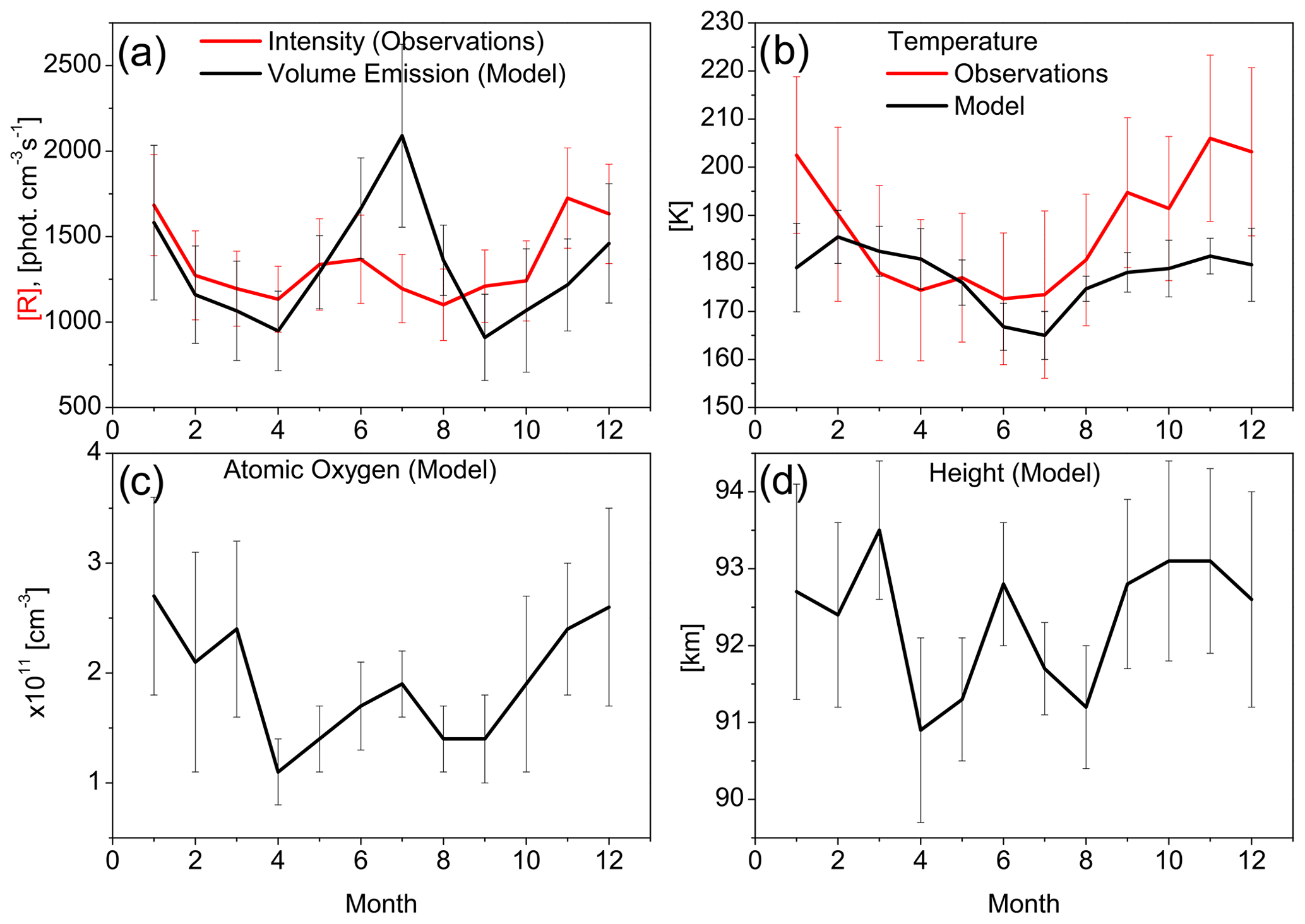
Figure 1 Observed at 43^∘ N (red line) and modelled at 43.75^∘ N (black line), annual variability of intensity and volume emission (a), temperature (b), atomic oxygen concentration (c), and height at the peak of the ${\mathrm{OH}}_{\mathit{\text{v}}=\mathrm{6}}^{\ast }$ layer.

3 Results and discussion

Figure 1a illustrates the nightly mean monthly averaged values of the observed annual variability of intensity at 43^∘ N (red line) and the modelled annual variability of volume emission at the peak of the OH^∗ layer at 43.75^∘ N (black line), both for transition ${\mathrm{OH}}_{\mathit{\text{v}}=\mathrm{6}}^{\ast }$ → ${\mathrm{OH}}_{\mathit{\text{v}}=\mathrm{2}}^{\ast }$. The error bar shows monthly SD, because we display monthly mean values, and SDs commonly exceed the errors of measurements. By the observations as well as by modelling, we can clearly see semi-annual variations of emissions with peaks in winter and summer. Note that the observed intensity is directly proportional to the vertical integral of the volume emissions; hence, they reveal similar variations and dependencies on surrounding conditions near the peak of the excited hydroxyl layer.

Grygalashvyly et al. (2014), Sonnemann et al. (2015), and Grygalashvyly (2015) have derived and confirmed through modelling that the concentration of excited hydroxyl (hence, volume emission and intensity) at peak is directly proportional to the product of the surrounding pressure (hence, it depends on altitude), atomic oxygen number density, and the negative power of temperature (Eq. A2 in the appendix). Thus, in order to infer the reasons for this semi-annual variation, one should consider three drivers of OH^∗ variability: temperature, atomic oxygen concentration, and height of the layer.

Figure 1b shows the monthly mean nightly averaged values of the observed annual variability of temperature at 43^∘ N (red line) and the modelled annual variability of temperature at the ${\mathrm{OH}}_{\mathit{\text{v}}=\mathrm{6}}^{\ast }$ peak at 43.75^∘ N (black line). Both the observations and the modelling show minima in summer and maxima in winter. Hence, the temperature decline can be one of the reasons for the summer intensity (and volume emission) peak.

Figure 1c and d depicts modelled monthly mean nightly averaged values of atomic oxygen at ${\mathrm{OH}}_{\mathit{\text{v}}=\mathrm{6}}^{\ast }$ peak and the height of the excited hydroxyl peak, respectively, at 43.75^∘ N. The modelling shows the peaks of atomic oxygen concentration in July and December–January, with the largest values in winter. The variation of height through the year occurs from ∼ 90 to 94 km. This is an essential variability and provides input to the variability of the concentration of the surrounding air.

In order to study the morphology of this semi-annual variation and assess the impacts of temperature, atomic oxygen concentration, and height (concentration of air) variability, we calculate 1-month sliding averaged values based on the model results. Figure 2 illustrates the modelled annual variability at the ${\mathrm{OH}}_{\mathit{\text{v}}=\mathrm{6}}^{\ast }$ peak: (a) volume emission (${\mathrm{OH}}_{\mathit{\text{v}}=\mathrm{6}}^{\ast }$ → ${\mathrm{OH}}_{\mathit{\text{v}}=\mathrm{2}}^{\ast }$), (b) temperature, (c) atomic oxygen concentration, and (d) height of the peak.

Figure 2 Nightly mean 1-month sliding average volume emission (a), temperature (b), atomic oxygen at peak of ${\mathrm{OH}}_{\mathit{\text{v}}=\mathrm{6}}^{\ast }$ (c), and height of peak of ${\mathrm{OH}}_{\mathit{\text{v}}=\mathrm{6}}^{\ast }$.

The summer maximum of volume emission (Fig. 2a) shows the strongest values in July and is extended from ∼ 30 to ∼ 50^∘ N. The summer maximum is stronger than that in winter. The winter maximum has its strongest values in January and a positive gradient into the winter pole direction; at latitudes 30–50^∘ N, it represents the part of the annual variation at high latitudes that occurs because of the annual variation in general mean circulation and fluxes of atomic oxygen which correspond to this variability (Liu et al., 2008; Marsh et al., 2006). Similar behaviour of the emissions for transition ${\mathrm{OH}}_{\mathrm{v}=\mathrm{8}}^{\ast }$ → ${\mathrm{OH}}_{\mathrm{v}=\mathrm{3}}^{\ast }$ was captured by WINDII (Wind Imaging Interferometer) and modelled by the Thermosphere-Ionosphere-Mesosphere Electrodynamics general circulation model at 84–88 km (Liu et al., 2008; Figs. 5 and 6).

The temperature (Fig. 2b) shows a clear annual variation from the middle to the high latitudes, with a minimum ∼ 150 K at middle latitudes in July. The summer minimum at the middle latitudes is the echo of the one at high latitudes. The atomic oxygen concentrations (Fig. 2c) reveal the annual cycle. The concentrations have a maximum in winter and a minimum in summer at high and middle latitudes, as has already been observed (Smith et al., 2010). However, in the region from ∼ 30 to ∼ 50^∘ N in summer, atomic oxygen concentrations show one additional peak in June–July. Formation of this summer peak can be explained by the transformed Eulerian mean (TEM) circulation (Limpasuvan et al., 2012; Fig. 7; Limpasuvan et al., 2016; Fig. 5), which brings into the summer hemisphere the air reached by atomic oxygen from the region of its production at high latitudes above 100 to ∼ 90 km at ∼ 30–50^∘ N. The peak altitude of the ${\mathrm{OH}}_{\mathit{\text{v}}=\mathrm{6}}^{\ast }$ peak (Fig. 2d) shows complex annual variability. There is a secondary maximum OH^∗ peak at ∼ 30–50^∘ N in summer.

In order to assess the input into annual variability from different sources, we calculate relative to annually averaged variations of volume emissions due to atomic oxygen, temperature, and air density:

$$\begin{array}{}\text{(2)}& \begin{array}{rl}& {\text{RD}}_{\mathrm{O}}^{\prime }=\mathrm{100}\mathit{\%}\cdot {\displaystyle \frac{V_{\mathrm{O}}^{\prime }}{\stackrel{\mathrm{‾}}{V}}}=\mathrm{100}\mathit{\%}\cdot {\displaystyle \frac{{\left[\mathrm{O}\right]}^{\prime }}{\stackrel{\mathrm{‾}}{\left[\mathrm{O}\right]}}},\\ & {\text{RD}}_T^{\prime }=\mathrm{100}\mathit{\%}\cdot {\displaystyle \frac{V_T^{\prime }}{\stackrel{\mathrm{‾}}{V}}}=\mathrm{100}\mathit{\%}\cdot -\mathrm{2.4}{\displaystyle \frac{T^{\prime }}{\stackrel{\mathrm{‾}}{T}}},\\ & {\text{RD}}_M^{\prime }=\mathrm{100}\mathit{\%}\cdot {\displaystyle \frac{V_M^{\prime }}{\stackrel{\mathrm{‾}}{V}}}=\mathrm{100}\mathit{\%}\cdot {\displaystyle \frac{{\left[M\right]}^{\prime }}{\stackrel{\mathrm{‾}}{\left[M\right]}}},\end{array}\end{array}$$

where overbar denotes annually averaged values, and prime denotes difference of actual (modelled or observed) values from annually averaged values (in our case this is the difference between nightly mean 1-month sliding averaged values (Fig. 2) and nightly mean annually averaged values). The derivation of these parameters is presented in the appendix. A similar approach can be useful for analysing emission variations due to GWs, PWs, and tides.

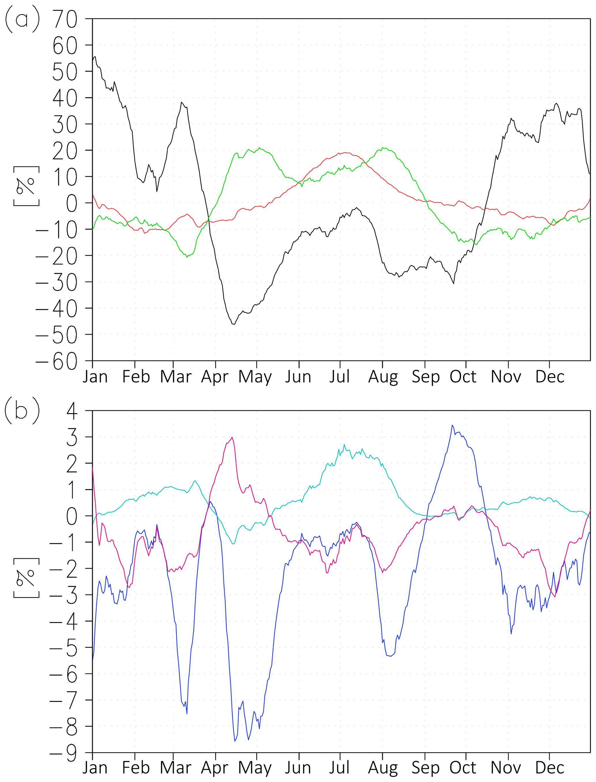
Figure 3 (a) Relative to annually averaged variations of volume emission (Eq. 2) due to atomic oxygen (black line), temperature (red line), and height (green line) at 43.75^∘ N. (b) Relative variations of volume emissions due to second momentum $\frac{{\left[\mathrm{O}\right]}^{\prime }{M}^{\prime }}{\stackrel{\mathrm{‾}}{\left[\mathrm{O}\right]}\stackrel{\mathrm{‾}}{M}}$ (blue line), $\frac{T^{\prime }{M}^{\prime }}{\stackrel{\mathrm{‾}}{T}\stackrel{\mathrm{‾}}{M}}$ (cyan line), and $\frac{{\left[\mathrm{O}\right]}^{\prime }{T}^{\prime }}{\stackrel{\mathrm{‾}}{\left[\mathrm{O}\right]}\stackrel{\mathrm{‾}}{T}}$ (magenta line) at 43.75^∘ N.

Figure 3a shows relative variations of emissions due to impacts of atomic oxygen (black line), temperature (red line), and air density (green line) at 43.75^∘ N. The strongest emission variation occurs because of changes in atomic oxygen concentration: the amplitude of its relative deviation amounts to ∼ 50 %. The amplitudes of relative deviations of emissions due to temperature and air density amount to ∼ 15 % and ∼ 20 %, respectively. The atomic oxygen variation gives the most essential input into the winter maximum of emission (black line). Because of the downward transport of atomic oxygen in winter, the volume emission rises by ∼ 50 % of annual average. The summer maximum is determined by the superposition of all three factors. After the spring reduction of emissions due to the decline of atomic oxygen concentration (∼ −40 % of annually averaged values), the emissions rise again to approximately the annual average values in June–July. This is synchronised with the growth of volume emissions by ∼ 20 % over the annual average values due to summer temperature declines (red line) and with the growth of volume emissions by ∼ 15 % over the annual average due to the decline of peak altitude in April–September and the corresponding rise of air density (green line).

Figure 3b illustrates relative variations of emissions due to second momenta (Eq. A7 in the appendix). The second momenta do not provide essential input to annual variation. The strongest among them, $\frac{{\left[\mathrm{O}\right]}^{\prime }{M}^{\prime }}{\stackrel{\mathrm{‾}}{\left[\mathrm{O}\right]}\stackrel{\mathrm{‾}}{M}}$ (blue line), gives emission variability with an amplitude of ∼ 6 % of annually averaged values.

In the context of our short paper, the ultimate question regarding the role of tides and GWs on semi-annual variations of OH^∗ emissions at middle latitudes has not been answered. Undoubtedly, the simultaneous analysis of observations of excited hydroxyl emissions from several stations is desirable to explore this question.

4 Summary and conclusions

Based on observations and numerical simulation, we confirmed the existence of a semi-annual cycle of excited hydroxyl emission at middle latitudes with maxima in summer (June–July) and winter (December–January). The annual variation in general mean circulation and atomic oxygen concentration corresponding to the excited hydroxyl emission cycle was found to be the leading cause of the winter maximum of this cycle, whereas the summer maximum represents the superposition of three different processes: atomic oxygen meridional transport due to residual circulation from the summer pole to the Equator; temperature decline, which represents the rest of the mesopause cooling at summer high latitudes; and air concentration growth at the peak of the excited hydroxyl emission layer due to hydroxyl layer descent at middle latitudes in April–September.

Appendix A

To obtain the derivation of Eq. (2), we start with a simplified equation for excited hydroxyl concentration. Taking into account that the ozone is in photochemical equilibrium in the vicinity of the [OH_v] layer and above during night-time (Kulikov et al., 2018a, 2019; Belikovich et al., 2018a); utilising the equation for ozone balance during night-time $\left(a_{\mathrm{5}}\left[{\mathrm{O}}_{\mathrm{3}}\right]\left[\mathrm{O}\right]+a_{\mathrm{1}}\left[\mathrm{H}\right]\left[{\mathrm{O}}_{\mathrm{3}}\right]=a_{\mathrm{4}}\left[\mathrm{O}\right]\left[{\mathrm{O}}_{\mathrm{2}}\right]\left[M\right]\right)$, where a₄ and a₅ are the coefficients for the corresponding reactions; omitting the reaction of atomic oxygen with ozone as relatively slow (Smith et al., 2008); substituting the reduced ozone balance equation for the excited hydroxyl balance equation (first term in the numerator of Eq. 1); assuming that the most effective production of excited hydroxyl occurs due to the reaction of ozone with atomic hydrogen and that the most effective losses are due to quenching with molecular oxygen; we obtain from Eq. (1) a simplified expression in which excited hydroxyl concentration is represented in terms of atomic oxygen concentration, temperature (in a₄), and concentration of the surrounding air:

$$\begin{array}{}\text{(A1)}& \left[{\mathrm{OH}}_v\right]\approx {\mathit{\mu }}_v{a}_{\mathrm{4}}\left[\mathrm{O}\right]\left[M\right].\end{array}$$

Here ${\mathit{\mu }}_v=\frac{{\mathit{\varsigma }}_v+{\sum }_{v^{\prime }=v+\mathrm{1}}^{v^{\prime }=\mathrm{9}}{\mathit{\mu }}_{v^{\prime }}{B}_{v^{\prime }v}}{{\sum }_{v^{\prime \prime }=\mathrm{0}}^{v^{\prime \prime }=v-\mathrm{1}}{B}_{v{v}^{\prime \prime }}},\left({\mathit{\varsigma }}_{v>\mathrm{9}}=\mathrm{0}\right)$ represents the coefficients representing the arithmetic combination of branching ratios ς_v and quenching coefficients $B_{v^{\prime }v}$. More comprehensive derivations of Eq. (A1) can be found in a number of papers (Grygalashvyly et al., 2014; Grygalashvyly, 2015; Grygalashvyly and Sonnemann, 2020). Although the accuracy of the Eq. (A1) estimate is insufficient for model calculations, it is useful for obtaining information about impacts and for assessing variabilities.

By multiplying Eq. (A1) by the Einstein coefficient $E_{v{v}^{\prime \prime }}$ for a given transition, writing the reaction rate explicitly $a_{\mathrm{4}}=\mathrm{6}\times {\mathrm{10}}^{-\mathrm{34}}(\mathrm{300}/T{)}^{\mathrm{2.4}}$ (Burkholder et al., 2015), and collecting all constants in ${\mathit{\chi }}_{v{v}^{\prime \prime }}$, we obtain an expression for volume emission in terms of atomic oxygen concentration, temperature, and air number density:

$$\begin{array}{}\text{(A2)}& V\approx {\mathit{\chi }}_{v{v}^{\prime \prime }}{T}^{-\mathrm{2.4}}\left[\mathrm{O}\right]\left[M\right],\end{array}$$

where ${\mathit{\chi }}_{v{v}^{\prime \prime }}={\mathit{\mu }}_v{E}_{v{v}^{\prime \prime }}\cdot \mathrm{6}\times {\mathrm{10}}^{-\mathrm{34}}\cdot {\mathrm{300}}^{\mathrm{2.4}}$.

Next, we apply Reynolds decomposition by averaged parts and variable parts to the temperature, atomic oxygen concentration, and concentration of air in Eq. (A2):

$$\begin{array}{}\text{(A3)}& V\approx {\mathit{\chi }}_{v{v}^{\prime \prime }}{\left(\stackrel{\mathrm{‾}}{T}+T^{\prime }\right)}^{-\mathrm{2.4}}\left(\stackrel{\mathrm{‾}}{\left[\mathrm{O}\right]}+{\left[\mathrm{O}\right]}^{\prime }\right)\left(\stackrel{\mathrm{‾}}{\left[M\right]}+{\left[M\right]}^{\prime }\right),\end{array}$$

where $\stackrel{\mathrm{‾}}{T}$, $\stackrel{\mathrm{‾}}{\left[\mathrm{O}\right]}$, and $\stackrel{\mathrm{‾}}{\left[M\right]}$ are average parts, and T^′, [O]^′, and [M]^′ are the corresponding varying parts.

After decomposing the term with temperature in the Taylor expansion and cross-multiplying all terms of Eq. (A3), we obtain

$$\begin{array}{}\text{(A4)}& \begin{array}{rl}V\approx & {\mathit{\chi }}_{v{v}^{\prime \prime }}{\stackrel{\mathrm{‾}}{T}}^{-\mathrm{2.4}}\stackrel{\mathrm{‾}}{\left[\mathrm{O}\right]}\cdot \stackrel{\mathrm{‾}}{\left[M\right]}+{\mathit{\chi }}_{v{v}^{\prime \prime }}{\stackrel{\mathrm{‾}}{T}}^{-\mathrm{2.4}}\stackrel{\mathrm{‾}}{\left[\mathrm{O}\right]}{\left[M\right]}^{\prime }\\ & +{\mathit{\chi }}_{v{v}^{\prime \prime }}{\stackrel{\mathrm{‾}}{T}}^{-\mathrm{2.4}}{\left[\mathrm{O}\right]}^{\prime }\stackrel{\mathrm{‾}}{\left[M\right]}-\mathrm{2.4}{\mathit{\chi }}_{v{v}^{\prime \prime }}{T}^{\prime }{\stackrel{\mathrm{‾}}{T}}^{-\mathrm{3.4}}\stackrel{\mathrm{‾}}{\left[\mathrm{O}\right]}\cdot \stackrel{\mathrm{‾}}{\left[M\right]}\\ & +{\mathit{\chi }}_{v{v}^{\prime \prime }}{\stackrel{\mathrm{‾}}{T}}^{-\mathrm{2.4}}{\left[\mathrm{O}\right]}^{\prime }{\left[M\right]}^{\prime }-\mathrm{2.4}{\mathit{\chi }}_{v{v}^{\prime \prime }}{T}^{\prime }{\stackrel{\mathrm{‾}}{T}}^{-\mathrm{3.4}}\stackrel{\mathrm{‾}}{\left[\mathrm{O}\right]}{\left[M\right]}^{\prime }\\ & -\mathrm{2.4}{\mathit{\chi }}_{v{v}^{\prime \prime }}{T}^{\prime }{\stackrel{\mathrm{‾}}{T}}^{-\mathrm{3.4}}{\left[\mathrm{O}\right]}^{\prime }\stackrel{\mathrm{‾}}{\left[M\right]}-\mathrm{2.4}{\mathit{\chi }}_{v{v}^{\prime \prime }}{T}^{\prime }{\stackrel{\mathrm{‾}}{T}}^{-\mathrm{3.4}}{\left[\mathrm{O}\right]}^{\prime }{\left[M\right]}^{\prime }.\end{array}\end{array}$$

The volume emission for a given transition can be represented as follows:

$$\begin{array}{}\text{(A5)}& \begin{array}{rl}V\approx & \stackrel{\mathrm{‾}}{V}+V_M^{\prime }+V_{\mathrm{O}}^{\prime }+V_T^{\prime }+V_{\mathrm{O}M}^{\prime \prime }+V_{TM}^{\prime \prime }+V_{T\mathrm{O}}^{\prime \prime }\\ & +\text{higher\hspace{0.17em} momenta},\end{array}\end{array}$$

where $\stackrel{\mathrm{‾}}{V}={\mathit{\chi }}_{v{v}^{\prime \prime }}{\stackrel{\mathrm{‾}}{T}}^{-\mathrm{2.4}}\stackrel{\mathrm{‾}}{\left[\mathrm{O}\right]}\cdot \stackrel{\mathrm{‾}}{\left[M\right]}$, $V_M^{\prime }={\mathit{\chi }}_{v{v}^{\prime \prime }}{\stackrel{\mathrm{‾}}{T}}^{-\mathrm{2.4}}\stackrel{\mathrm{‾}}{\left[\mathrm{O}\right]}{\left[M\right]}^{\prime }$, $V_{\mathrm{O}}^{\prime }={\mathit{\chi }}_{v{v}^{\prime \prime }}{\stackrel{\mathrm{‾}}{T}}^{-\mathrm{2.4}}{\left[\mathrm{O}\right]}^{\prime }\stackrel{\mathrm{‾}}{\left[M\right]}$, $V_T^{\prime }=-\mathrm{2.4}{\mathit{\chi }}_{v{v}^{\prime \prime }}{T}^{\prime }{\stackrel{\mathrm{‾}}{T}}^{-\mathrm{3.4}}\stackrel{\mathrm{‾}}{\left[\mathrm{O}\right]}\cdot \stackrel{\mathrm{‾}}{\left[M\right]}$, $V_{\mathrm{O}M}^{\prime \prime }={\mathit{\chi }}_{v{v}^{\prime \prime }}{\stackrel{\mathrm{‾}}{T}}^{-\mathrm{2.4}}{\left[\mathrm{O}\right]}^{\prime }{\left[M\right]}^{\prime }$, $V_{TM}^{\prime \prime }=-\mathrm{2.4}{\mathit{\chi }}_{v{v}^{\prime \prime }}{T}^{\prime }{\stackrel{\mathrm{‾}}{T}}^{-\mathrm{3.4}}$ $\stackrel{\mathrm{‾}}{\left[\mathrm{O}\right]}{\left[M\right]}^{\prime }$, and $V_{T\mathrm{O}}^{\prime \prime }=-\mathrm{2.4}{\mathit{\chi }}_{v{v}^{\prime \prime }}{T}^{\prime }{\stackrel{\mathrm{‾}}{T}}^{-\mathrm{3.4}}{\left[\mathrm{O}\right]}^{\prime }\stackrel{\mathrm{‾}}{\left[M\right]}$.

Hence, relative deviations (RDs) of emissions due to variations in atomic oxygen, temperature, and concentration of air are

$$\begin{array}{}\text{(A6)}& \begin{array}{rl}& {\text{RD}}_{\mathrm{O}}^{\prime }=\mathrm{100}\mathit{\%}\cdot {\displaystyle \frac{V_{\mathrm{O}}^{\prime }}{\stackrel{\mathrm{‾}}{V}}}=\mathrm{100}\mathit{\%}\cdot {\displaystyle \frac{{\left[\mathrm{O}\right]}^{\prime }}{\stackrel{\mathrm{‾}}{\left[\mathrm{O}\right]}}},\\ & {\text{RD}}_T^{\prime }=\mathrm{100}\mathit{\%}\cdot {\displaystyle \frac{V_T^{\prime }}{\stackrel{\mathrm{‾}}{V}}}=\mathrm{100}\mathit{\%}\cdot -\mathrm{2.4}{\displaystyle \frac{T^{\prime }}{\stackrel{\mathrm{‾}}{T}}},\\ & {\text{RD}}_M^{\prime }=\mathrm{100}\mathit{\%}\cdot {\displaystyle \frac{V_M^{\prime }}{\stackrel{\mathrm{‾}}{V}}}=\mathrm{100}\mathit{\%}\cdot {\displaystyle \frac{{\left[M\right]}^{\prime }}{\stackrel{\mathrm{‾}}{\left[M\right]}}}.\end{array}\end{array}$$

The relative deviations (RDs) of emissions due to second momenta are

$$\begin{array}{}\text{(A7)}& \begin{array}{rl}& {\text{RD}}_{\mathrm{O}M}^{\prime \prime }=\mathrm{100}\mathit{\%}\cdot {\displaystyle \frac{V_{\mathrm{O}M}^{\prime \prime }}{\stackrel{\mathrm{‾}}{V}}}=\mathrm{100}\mathit{\%}\cdot {\displaystyle \frac{{\left[\mathrm{O}\right]}^{\prime }{\left[M\right]}^{\prime }}{\stackrel{\mathrm{‾}}{\left[\mathrm{O}\right]}\stackrel{\mathrm{‾}}{\left[M\right]}}},\\ & {\text{RD}}_{TM}^{\prime \prime }=\mathrm{100}\mathit{\%}\cdot {\displaystyle \frac{V_{TM}^{\prime \prime }}{\stackrel{\mathrm{‾}}{V}}}=\mathrm{100}\mathit{\%}\cdot -\mathrm{2.4}{\displaystyle \frac{T^{\prime }{\left[M\right]}^{\prime }}{\stackrel{\mathrm{‾}}{T}\stackrel{\mathrm{‾}}{\left[M\right]}}},\\ & {\text{RD}}_{T\mathrm{O}}^{\prime \prime }=\mathrm{100}\mathit{\%}\cdot {\displaystyle \frac{V_{T\mathrm{O}}^{\prime \prime }}{\stackrel{\mathrm{‾}}{V}}}=\mathrm{100}\mathit{\%}\cdot -\mathrm{2.4}{\displaystyle \frac{T^{\prime }{\left[\mathrm{O}\right]}^{\prime }}{\stackrel{\mathrm{‾}}{T}\stackrel{\mathrm{‾}}{\left[\mathrm{O}\right]}}}.\end{array}\end{array}$$