the Creative Commons Attribution 4.0 License.
the Creative Commons Attribution 4.0 License.
 | 10 Sep 2020
The very low-frequency transmitter radio wave anomalies related to the 2010 Ms 7.1 Yushu earthquake observed by the DEMETER satellite and the possible mechanism
Shufan Zhao
XuHui Shen
Zeren Zhima
Chen Zhou
Earthquakes may disturb the lower ionosphere through various coupling mechanisms during the seismogenic and coseismic periods. The VLF (very low-frequency) signal radiated from ground-based transmitters will be affected when it penetrates the disturbed ionosphere above the epicenter area, and this anomaly can be recorded by low-Earth orbit satellites under certain conditions. In this paper, the temporal and spatial variation of the signal-to-noise ratio (SNR) of the VLF transmitter signal in the ionosphere over the epicenter of 2010 Yushu Ms 7.1 earthquake in China is analyzed using DEMETER (Detection of Electro-Magnetic Emission Transmitted from Earthquake Regions) satellite observation. The results show that SNR over the epicenter of the Yushu earthquake especially in the southwestern region decreased (or dropped) before the main shock, and a GPS–TEC (Global Positioning System; total electron content) anomaly accompanied, which implies that the decrease in SNR might be caused by the enhancement of TEC. A full-wave method is used to study the mechanism of the change in SNR before the earthquake. The simulated results show SNR does not always decrease before an earthquake. When the electron density in the lower ionosphere increases by 3 times, the electric field will decrease about 2 dB, indicating that the disturbed-electric-field decrease of 20 % compared with the original electric field and vice versa. It can be concluded that the variation of electron density before earthquakes may be one of the important factors influencing the variation of SNR.
- Article
(7196 KB) - Full-text XML
- BibTeX
- EndNote


The VLF (very low-frequency) radio waves radiated by the powerful ground-based VLF transmitters have been used for long-distance communication and submarine navigation because of the efficient reflection within the Earth–ionosphere waveguide. However, there is still a small fraction of the wave energy that can leak into the higher ionosphere and magnetosphere after being absorbed intensively by the lower ionosphere. The signals from transmitters observed by the LEO (low-Earth orbit) satellites can be used to study the propagation of VLF waves in the Earth–ionosphere waveguide and ionosphere, as well as wave–particle interaction in the radiation belt (Inan et al., 2007; Inan and Helliwell, 1982; Lehtinen and Inan, 2009; Parrot et al., 2007).
It is gradually confirmed that earthquake precursors not only appear near the ground but also may couple with the atmosphere and ionosphere through some mechanisms, resulting in plasma disturbances in the ionosphere and recorded by various instruments like ionosonde or GPS (Global Positioning System) receivers measuring TEC (total electron content) (Liu et al., 2009, 2001, 2006; Pulinets et al., 2000; Stangl et al., 2011; Zhao et al., 2008). Therefore, the amplitude of the VLF signals from the ground-based VLF transmitter observed on the ground and from satellites will change when encounter the disturbed area in the ionosphere (Hayakawa, 2007; Maurya et al., 2016; Molchanov et al., 2006; Píša et al., 2013). Molchanov et al. (2006) have found the signal-to-noise ratio (SNR) of the electric field from VLF transmitters recorded by the DEMETER (Detection of Electro-Magnetic Emission Transmitted from Earthquake Regions) satellite decreased near the epicenters during a series of earthquakes. The spatial size of an SNR reduction zone increases with the magnitude of the earthquake. However, it is hard to distinguish the coseismic anomaly and precursor from their results.
Two devastating earthquakes, the 2008 Ms 8.0 Wenchuan earthquake and the 2010 Ms 7.1 Yushu earthquake, occurred successively in southwestern China during the operation period (2004–2010) of the DEMETER satellite. Some research have also focused on the SNR variation of VLF transmitters using DEMETER satellite observation to extract the earthquake-related anomalies before the two strong earthquakes (He et al., 2009; Shen et al., 2017; Yao et al., 2013). The results all illustrated the decrease in SNR before the earthquakes. Since the earthquake-related ionospheric disturbance zone is not right over the epicenter, the relative position of the SNR anomaly and the epicenter should be further studied. The factors which influence SNR and the possible mechanism also needs to be comprehensively illustrated.
The Alpha VLF transmitters in Russia transmit three frequencies in each station which provide us opportunities to study the influence of the ionosphere on different wave frequencies. The devastating earthquake nearest the transmitters in China is the 2010 Ms 7.1 Yushu earthquake. In this paper we investigate the temporal and spatial SNR variation of the VLF transmitter signal in the ionosphere near the epicenter of the Yushu earthquake using DEMETER observation. The background variations of SNR in the same period of 2007–2010 have also been studied to distinguish whether the SNR reduction is caused by an earthquake or just ionospheric background changes. The mechanism of how the seismo-ionospheric disturbance affects the variation of SNR is discussed in this paper.
Regarding the mechanism of the VLF radio wave variations in the altitude of a LEO satellite (presented as SNR variation) before the earthquakes, Hayakawa (2007) and Píša et al. (2013) suggest the VLF anomalies exist because the lower ionosphere is lowered before earthquake. Molchanov et al. (2006) declared that the variation of SNR of satellite data is attributed to the ionospheric disturbance, especially the lower-ionospheric disturbance. Furthermore, it has been found that the electron density variation could exist in the lower ionosphere according to the computer ionosphere tomography (CIT) results based on GPS–TEC data before the Nepal Ms 8.1 earthquake in 2015 (Kong et al., 2018). The electric-field-penetrating model has shown that the electron density and height of the lower ionosphere can be changed by the additional current in the global electric circuit before the earthquake. On the other hand, Marshall et al. (2010) construct a 3D finite-difference time domain model to simulate that lightning could also cause the disturbance of the electron density in the lower ionosphere, which has a similar mechanism to the earthquake. Many studies also have found that the main loss of VLF wave power mainly occurs in the D–E region of the ionosphere when the wave penetrates into the ionosphere (Cohen and Inan, 2012; Liao et al., 2017; Starks et al., 2008; Tao et al., 2010; Zhao et al., 2017, 2015). In sum, the electron density variation in the lower ionosphere might be one main factor causing the SNR anomaly of VLF transmitter signal in the ionosphere. Based on these results, the full-wave calculation model was utilized to study the influence of the electron density disturbance of the lower ionosphere on the variation of VLF radio signals.
In this paper, a brief description of the DEMETER data and full-wave method used in this study are presented in Sect. 2. The temporal and spatial variations of SNR over the epicenter have been investigated before the Yushu earthquake with 4 years (2007–2010) of data; the full-wave model is used to simulate how the variation of electron density in the lower ionosphere affects the SNR of the electric field from a VLF transmitter at the altitude of a satellite in Sect. 3. The discussion and conclusions of this study are presented in Sects. 4 and 5 separately.
2.1 Earthquake, VLF transmitters, and DEMETER data
At the local time of 07:49:37.9 on 14 April 2010, a Ms 7.1 earthquake hit the city of Yushu, Qinghai province, with an epicenter at 33.2∘ N, 96.6∘ E and a 14 km depth in the northeastern Tibetan Plateau. The nearest VLF transmitter around the epicenter is in the proximity of Novosibirsk (NOV), which belongs to the Russian Alpha navigation system consisting of three transmitters. The other two transmitters named Krasnodar (KRA) and Khabarovsk (KHA) are far away from the Yushu earthquake, so only the satellite data radiated from NOV have been used for analysis in this paper. The location of the transmitters and the epicenter of the Yushu earthquake are denoted by blue squares and black stars, respectively, in Fig. 1. Each transmitter radiates three different frequency VLF radio signals (11.9, 12.6, and 14.9 kHz), with a 0.4 s duration and a 3.6 s cycle.
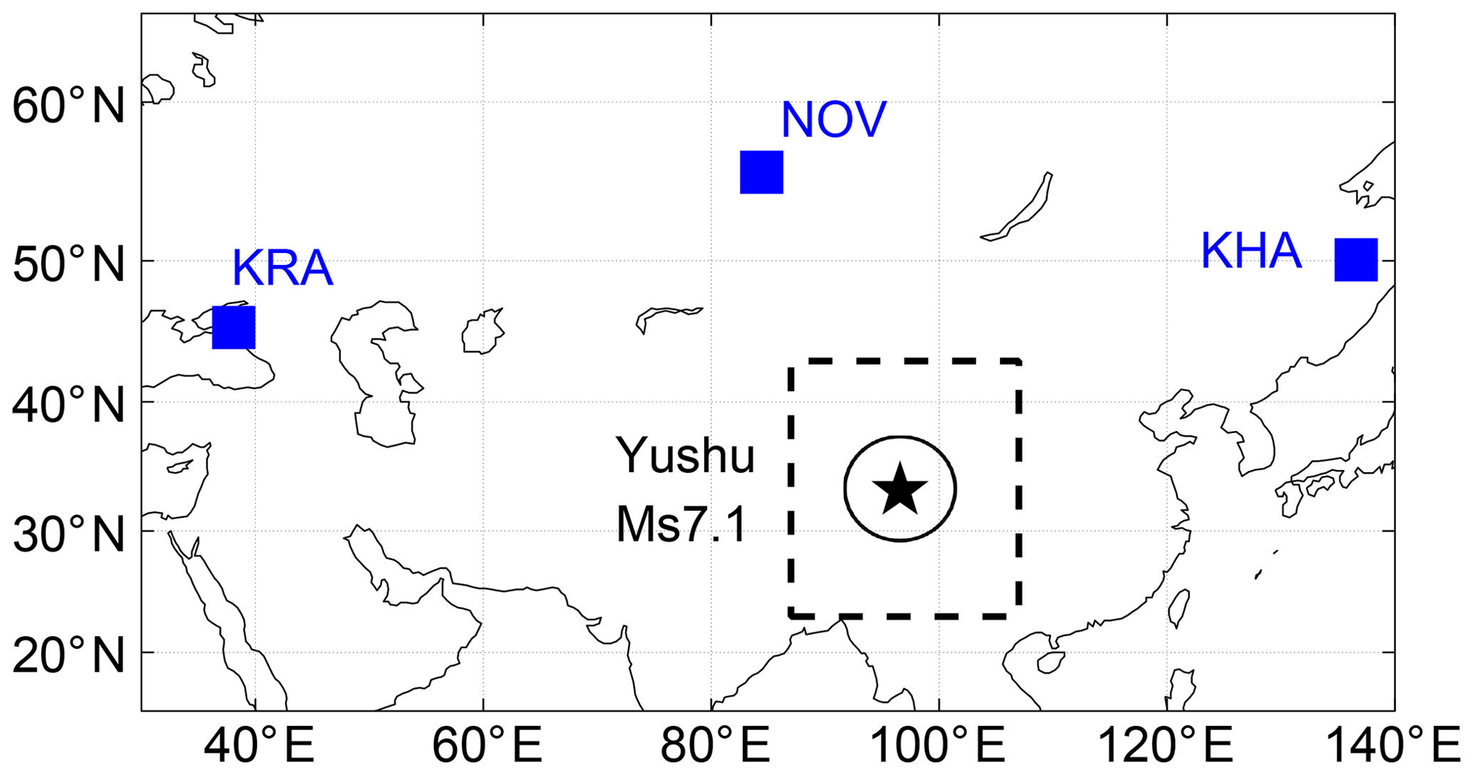
Figure 1The locations of transmitters and the Yushu earthquake. The blue squares represent the locations of the three transmitters (KRA, NOV, and KHA) in Russia. The epicenter of Yushu earthquake is denoted by the black star. The black square covers the region of the epicenter , in which the data have been studied.
The DEMETER satellite was launched on 29 June 2004 as a sun-synchronous orbit at an altitude of 710 km, which then was changed to 660 km in December 2005 (Parrot et al., 2006), and the operation was ended in December 2010. The scientific objective of DEMETER is to detect and characterize the electromagnetic signals associated with natural phenomena (such as earthquakes, volcanic eruptions, and tsunamis) or anthropogenic activities. It operated in the region from invariant latitude −65 to 65∘, with descending and ascending orbits crossing the Equator at the local time of ∼10:00 and ∼22:00, respectively. DEMETER has a revisit orbit period of about 14 d, which means the satellite returns over the same orbit trajectory after 13 d. The payloads include several electromagnetic sensors with two working mode: burst and survey. At the ELF–VLF (extremely low-frequency) band, the intensive-electromagnetic-wave data over locations of particular interest were provided in the burst mode, and in the survey mode, electric and magnetic power spectral density (PSD) data every 2 s were provided with a sampling frequency of 40 kHz and spectral resolution of 19.53 Hz.
According to the formula of Dobrovolsky et al. (1979) the preparation zone of the earthquake can reach ρ=100.43M, where M is the magnitude of the earthquake and ρ is measured in kilometers. Considering the limited extension of the Ms 7.1 Yushu earthquake, the preparation zone ρ can reach to 1130 km; we mainly focused on the region within the region of the epicenter (black square in Fig. 1). In this study, the nighttime PSD data of the electric field from the DEMETER's survey mode observations were extracted study the perturbations of the VLF signal before and after the Yushu earthquake. As the VLF radio signals at daytime are too small to cause obvious SNR variation compared with those at nighttime, we did not use the daytime data in this study.
2.2 The method to calculate SNR
According to the method of Molchanov et al. (2006), the SNR of the electric field was calculated as follows:
where A(f0) is the amplitude of the electric-field spectrum at the central frequency and A(f±) values are the spectrums at , where Δf is the chosen frequency band. For the three Russian VLF transmitters, the f0 is set as three VLF radio waves frequency radiated from NOV transmitters at 11.9, 12.6, and 14.9 kHz and the Δf=300 Hz.
2.3 Full-wave method
A full-wave method has been used to seek a solution of Maxwell equations for waves varying as ejωt in a horizontally stratified medium with fixed dielectric permittivity tensors and permeability μ in each layer. Considering the region of our interest is much smaller than the radius of the earth, the earth's curvature is neglected in this study. A Cartesian coordinate system is established with x, y in the horizontal plane and z as vertical upward. We seek a solution of the Maxwell equations in the form of a linear combination of plane waves , where kbot is the horizontal component of the wave vector k, which is conserved by Snell's law inside each layer; we have
where ω is the angular frequency, μ is the permeability of the medium (µ≡1 for nonmagnetic medium), is dielectric tensor, and is electric-susceptibility tensor (Yeh and Liu, 1972). is determined by the electron density and collision frequency in the ionosphere, as well as the geomagnetic field. In our simulation, the electron density is calculated by the International Reference Ionosphere (IRI) model (Bilitza et al., 2017), and the electron collision frequency (denoted by v) is modeled by the exponential-decay law with the height (denoted by h) increasing at . The parameters of the geomagnetic field at the location of the VLF transmitter is calculated by the International Geomagnetic Reference Field (IGRF) model (Finlay et al., 2010).
Eliminating the z components from Eq. (1), we can obtain the following elegant form of Maxwell equations.
where V=(EbotZ0Hbot), Z0 is wave impedance and is a 4×4 matrix:
The electromagnetic field in each layer can be obtained in the k (wave vector) domain by solving Eq. (2) recursively in a direction which provides stability against numerical “swamping” (Budden, 1985; Lehtinen and Inan, 2008). The difficulty is how to deal with numerical stability when the solution of evanescent waves “swamp” the waves of interest because of the large imaginary vertical-wave number. More details of the full-wave method are described in Lehtinen and Inan (2008).
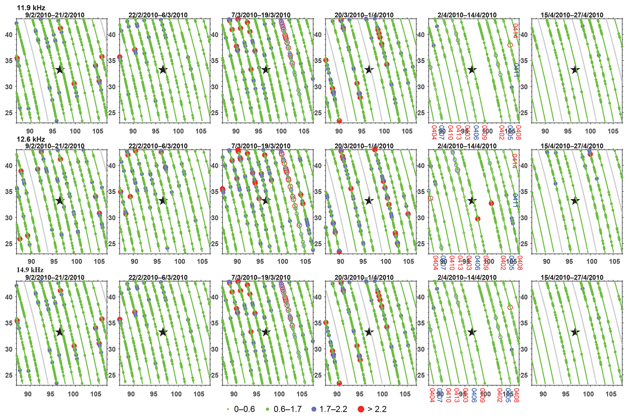
Figure 2The evolution of SNR evolution VLF radio waves frequencies 11.9 kHz (top panel), 12.6 kHz (middle panel), 14.9 kHz (bottom panel) with Δf=300 Hz at nighttime. The black star stands for the epicenter of the Yushu earthquake; the gray line represents the transmitter that turns off on that day; the days with high geomagnetic activity are marked by blue and hollow dots. Please note that the date format of the black text in this figure is day-month-year, but the date format of the red and blue text is month day.
3.1 VLF signal analysis from the DEMETER satellite
The SNR five revisit periods before and one revisit period after the earthquake in 2010 were calculated to study the evolution of SNR above the epicenter. The SNR distributions of three frequencies (11.9, 12.6, and 14.9 kHz) within the region of the epicenter are shown in Fig. 2, where the value of SNR is denoted with colored dots with different sizes and the black star represents the epicenter of the Yushu earthquake. The data during geomagnetic storms (here we defined Kp > 3 and Dst < −30 nT) were plotted with hollow dots, and very small gray dots mean that the transmitter is turned off on these days. It can be found that in the first revisit period (2–14 April) before the earthquake, the SNRs of the three frequencies all decrease dramatically compared with other periods no matter whether it is before or after the earthquake. In the first revisit period from 2 to 14 April in 2010, two magnetic storms occurred on 4–7 and 11–12 April, respectively.
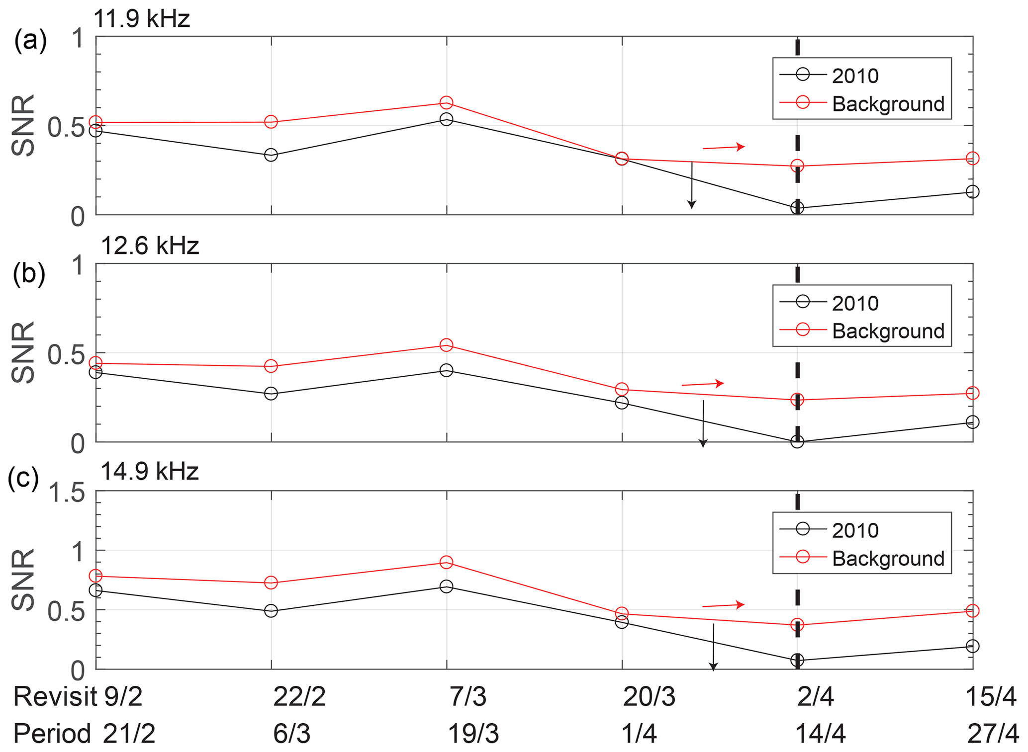
Figure 3The average SNR variation with revisit periods inside the square region with the center of the epicenter. Panels (a–c) show SNR at 11.9, 12.6, and 14.9 kHz and the numbers of the averaged data points. The green and red lines represent the SNR variations in 2010 and background time separately. The black dashed line represents the period with the end date of the main-shock date.
To minimize the impact of other factors and confirm whether the SNR anomaly is caused by the earthquake and not the variation of the ionospheric background, we focus on SNR in the black square (shown in Fig. 1) of the same period in 2007–2009 as the background, when there are no large earthquakes and the data when the transmitter was turned off or affected by geomagnetic storms are eliminated. The mean value of all the data in each period has been obtained to get the time sequence shown in Fig. 3. In Fig. 3, the black dashed line represents the occurrence date of the earthquake. The black and red solid lines represent the average values in the five periods before the earthquake and one period after the earthquake within the region of the epicenter in 2010 and background time, respectively. The change trends of SNR in the background time and 2010 are the same except in the first period before the earthquake. In the first period before the earthquake SNR decreased significantly in 2010, while it increased in background time at all transmitting frequencies. It means that the decrease in SNR in the first period in 2010 might be caused by Yushu earthquake.
The above results use the average value within the region of the epicenter in one revisit period of DEMETER to analyze the anomalies which ignore the day-to-day variability of the ionosphere. Furthermore, the daily variation of SNR in the first period before the earthquake is studied using a quartile-based process (Liu et al., 2009) to detect the anomaly of SNR. The median (M), the lower (first) quartile (denoted as LQ), and the upper (third) quartile (UQ) of every successive 11 d of SNR of the orbit data within the region of the epicenter have been calculated to find the deviation between the observed SNR of the 12th day and the computed median (M). Based on the assumption of the normal distribution of SNR with the mean (m) and standard deviation (σ), the expected value of M and LQ or UQ are equal to m and 1.34σ (Liu et al., 2009, and references therein). We set the lower boundary (LB in short) to LB = M + 2(M-LQ) and the upper boundary (UB) to UB = M + 2(UQ-M) to find the SNR anomalies with a stricter criterion. Thus, if an observed SNR on the 12th day is greater or smaller than its previous 11 d based on UB or LB, a positive or negative anomaly of SNR will be identified. Figure 4 shows the time series of SNR at 11.9, 12.6, and 14.9 kHz, and the red, gray, black curves denote the current SNR, associated median, and upper and lower boundary (UB and LB), respectively. Blue and green markers represent the positive and negative anomaly. As shown in Fig. 4, besides the negative anomalies which appeared on 13 April (1 d before the Yushu earthquake; the occurrence time of the Yushu earthquake is denoted by a vertical dashed line in Fig. 4) at all transmitting frequencies, another three anomalies occurred on 29 March, 8 April, and 10 April, respectively. Previous research indicates that earthquake anomalies usually occurred within 1 week before an earthquake, so the negative anomaly which occurred on 29 March at 12.6 and 14.9 kHz may be not related to the Yushu earthquake. The anomalies on 8 and 10 April only occurred on one single transmitting frequency, which may not be significant and is needed to be further researched.
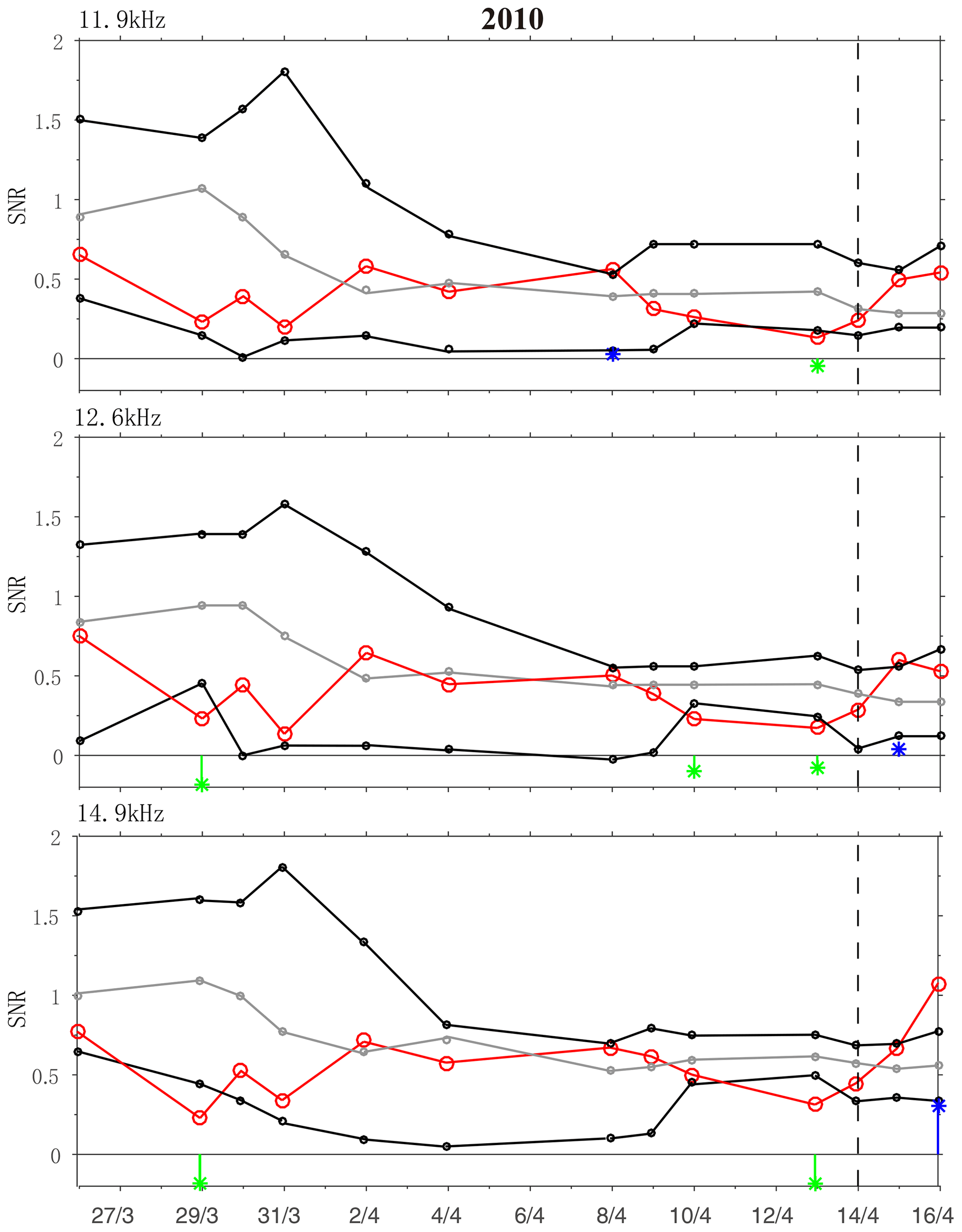
Figure 4A time series of SNR right above the Yushu epicenter. The Ms 7.1 Yushu earthquake occurred at the local time of 07:49:37.9 on 14 April 2010. The red, gray, and two black curves denote the currently observed SNR, associated median, and upper and lower bound (UB and LB), respectively. Blue and green sign represent the upper and lower anomalous days identified by the computer routine, respectively. The LB and UB are constructed by the previous 1–11 d moving median (M), lower quartile (LQ), and upper quartile (UQ), and the LB and UB are calculated by LB = M + 2(M-LQ) and UB = M + 2(UQ-M).
The result in Fig. 4 shows the anomalies of SNR during the successive 20 d before the Yushu earthquake. However, the 20 d orbital data may be carried into the ionospheric background noise of different space. To avoid this kind of ionospheric background noise, we select the three revisit orbits to analyze the anomalies of SNR before the Yushu earthquake further (the revisit orbit on 9 April overhead the epicenter, the revisit orbit on 13 April which is 550 km away from epicenter, and the revisit orbit on 10 April which is 750 km away from the epicenter are selected). The quartile-based process is also performed for every revisit's orbital data, but the 6 d sliding-mean value (including 3 d before the current day and 2 d after the current day) have been analyzed. The green and blue bar represent negative and positive anomalies in one orbit, respectively, in Fig. 5. As we can see in the top and middle panel, on 9 and 10 April, the negative and positive anomalies both occurred like other days in the same two revisit orbits. These anomalies could be induced by the daily variation. In the bottom panel, there are no obvious anomalies in other days with the same revisit orbit of 13 April, but the SNR values have obvious negative anomalies for all orbits on 13 April. These results further confirm that the anomalies of SNR occurred on 13 April.
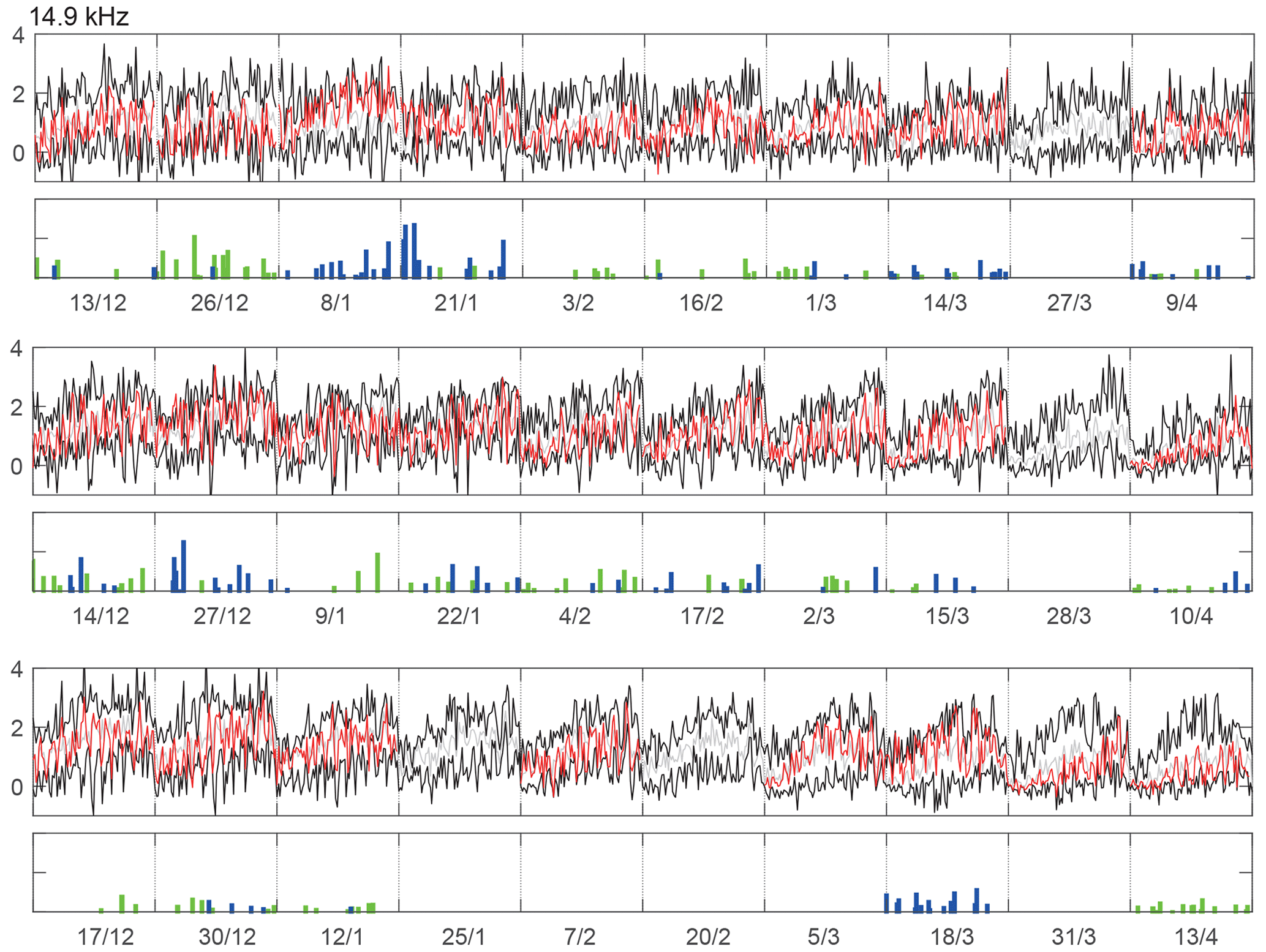
Figure 5A revisit orbital SNR of 9, 10, and 13 April 2010. The red, gray, and two black curves denote the currently observed SNR, associated median, and upper and lower bound (UB and LB), respectively. Blue and green bars represent the positive and negative anomalies in one orbit, respectively. The LB and UB are constructed by the 6 d moving median (M, including 3 d before the current day and 2 d after the current day), lower quartile (LQ), and upper quartile (UQ), and the LB and UB are calculated by LB = M + 2(M-LQ) and UB = M + 2(UQ-M).
We speculate that the anomalies of SNR may be related to the anomalies of electron density. To confirm our conjecture, we used GPS–TEC map data distributed by CODE (Center for Orbit Determination in Europe) to check out whether the total electron content (TEC) showed similar anomalies. The resolution of TEC data from CODE is . We use 11 d sliding-mean values of every grid as a background, and then we can get a spatial distribution of the background. The background stand deviation is set as the threshold (upper bound and lower bound) to determine whether there are anomalies; if the intraday value exceeds the threshold, there are anomalies. We have reviewed the TEC anomalies of every day from 2 to 14 April (which means the duration of the sliding background is from 22 March to 13 April). The TEC anomalies only occurred on 13 April. The anomalies that are the most intensive were at 06:00 UT, which means only the SNR anomaly on 13 April is a possible earthquake precursor. The other two anomalies on 8 and 10 April in Fig. 4 may be caused by other factors. Figure 6a–b shows the TEC at 06:00 UT on 13 April and the sliding mean of the background (2–12 April); Fig. 6c–d shows the abnormal region where the TEC value exceeded the threshold (background standard deviation). As we can see, TEC had an abnormal enhancement on 13 April at the southwestern region of the epicenter. In addition, we collect the Constellation Observing System for Meteorology, Ionosphere and Climate (COSMIC) data in the abnormal region of TEC (southwestern region of the Yushu epicenter) to check whether there is abnormal variation in the D–E region electron density. As shown in Fig. 7, the result shows there indeed exists a disturbance in the E region on 13 April. Similar to the abnormal region of electron density, the SNR of orbit no. 030939-1 on 13 April also decreased in the southwestern direction in Fig. 2. This phenomenon may illustrate the decrease in SNR caused by TEC enhancement. Furthermore, this TEC enhancement was probably caused by an earthquake because it shows very intensive conjugate response. However, TEC anomalies caused by geomagnetic storms do not exhibit this kind of phenomenon generally (Zhao et al., 2008).
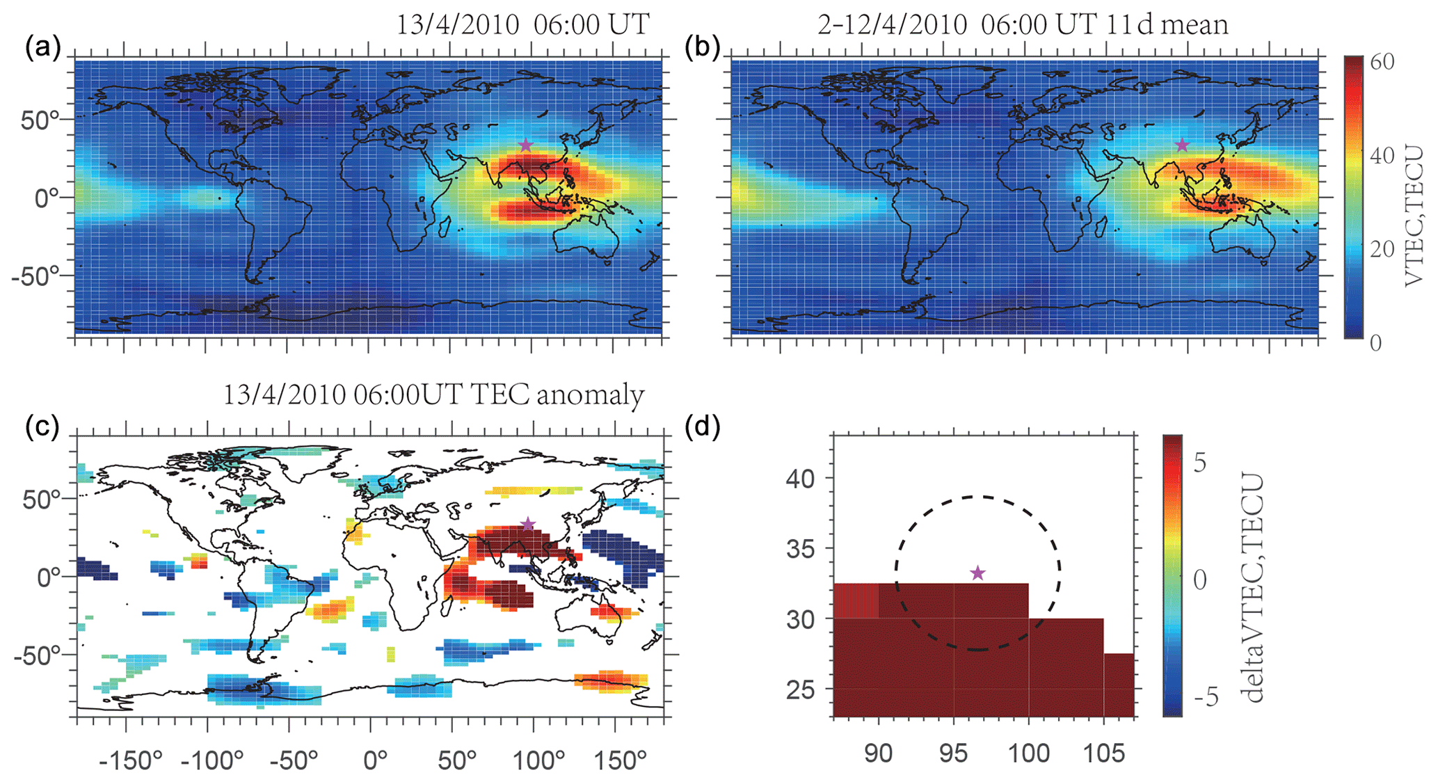
Figure 6The spatial distribution of the GPS–TEC map (a, b) and its anomalies (c, d). The GPS–TEC map on 13 April at 06:00 UT (a). The sliding mean of 11 d of background (b). The global anomalies in the GPS–TEC map (c). The regional anomalies around the epicenter of the Yushu earthquake in the GPS–TEC map (d). The purple pentagram indicates the epicenter, and the radius of the black circle is 550 km.
3.2 The possible mechanism of SNR variation revealed by full-wave simulation
In Sect. 3.1, we analyzed the spatial and temporal characteristics of SNR during the five revisit periods before and one revisit period after the Yushu earthquake. It can be found that SNR decreased significantly before the earthquake over the epicenter area of the Yushu earthquake, especially in the southwestern direction. After excluding the influence of geomagnetic storms, we further explored the possible mechanism of SNR abnormal variation in this section. As mentioned in the Sect. 1, the electron density in the lower ionosphere can be disturbed through various mechanisms before earthquakes. The electron density before the Nepal earthquake was obtained from a computer ionosphere tomography method by using GPS data (Kong et al., 2018). Their results shows that the abnormal variation of electron density occurred at a height of 150 km before the Nepal earthquake and the range of variation reached about 30 %. However the electron density hardly changed at a height of 450 km. Marshall et al. (2010) have shown that 60 horizontal discharge pulses of 7 V m−1 near the ground can cause 50 % change in electron density in the lower ionosphere, and 60 horizontal discharge pulses of 10 V m−1 near the ground can even cause a 400 % change in electron density. The variation of electron density in the ionosphere caused by lightning activity and an earthquake can both be explained by one lithosphere–atmosphere–ionosphere coupling mechanism with penetration of the direct current (DC) electric field (Zhou et al., 2017; Kuo et al., 2011). These results provide us a reference for the amplitude of the perturbation of the electron density in the D–E region. Based on these results, the full-wave model was used to simulate the changes in the electric field at satellite altitude excited by ground-based VLF transmitters caused by the enhancement of or decrease in electron density in the lower ionosphere so as to further determine the change law of SNR.
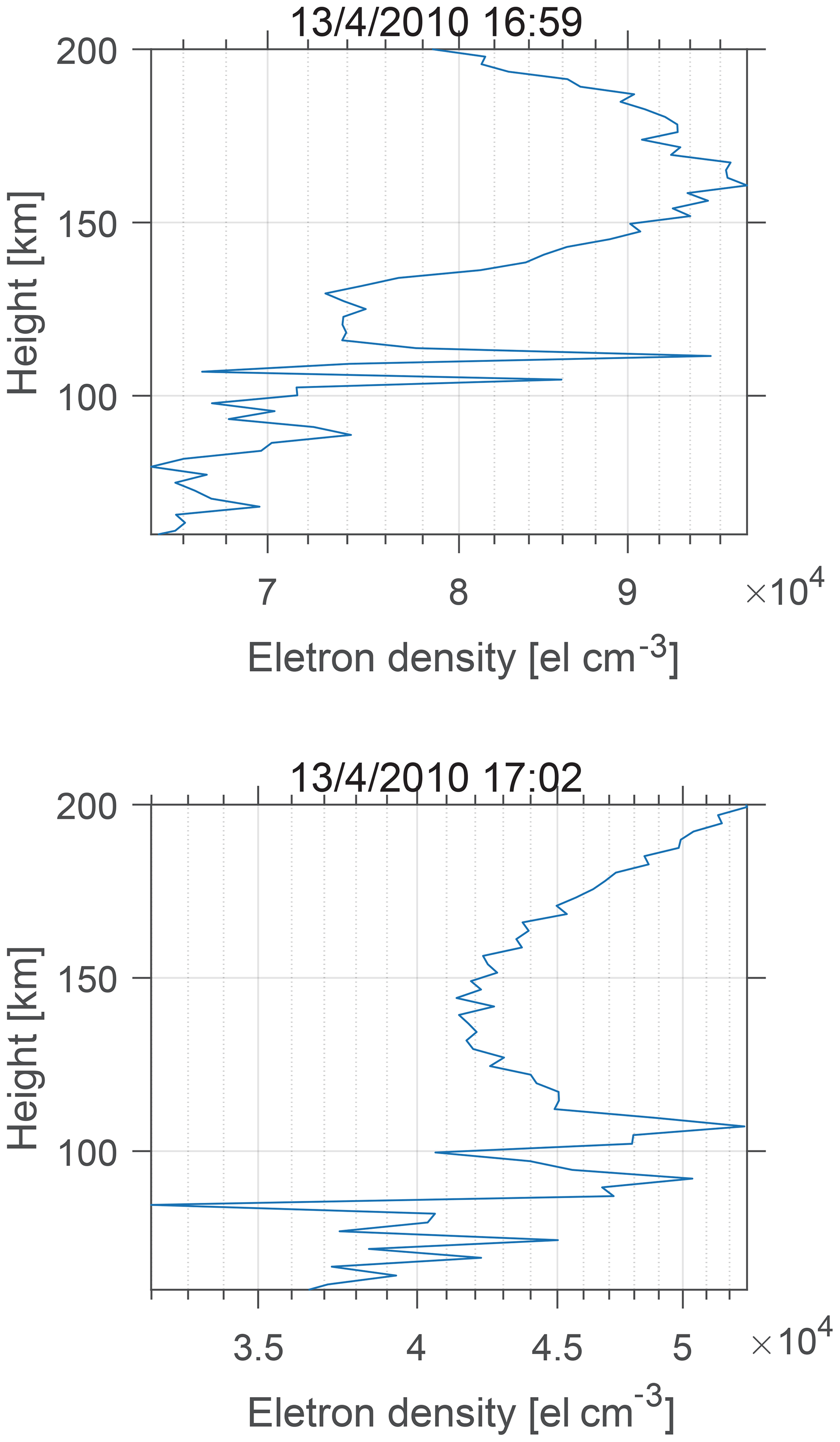
Figure 7The electron density obtained from COSMIC data on 13 April in the TEC abnormal region.
As mentioned in the introduction, the major VLF wave energy almost lost in the D–E region; after that, the radio waves penetrate the topside of the ionosphere and even magnetosphere with a minor linear reduction because of the mode conversion (Lehtinen and Inan, 2009; Shao et al., 2012). The data of COSMIC also illustrate that the anomaly of electron density not only occurred in the F region (represented by the anomaly of TEC) but also occurred in the D–E region, so the full-wave method (FWM) (Lehtinen and Inan, 2009) was utilized to simulate the electric field between altitudes of 0 and 120 km induced by the NOV transmitter, which is the closest transmitter to the epicenter of the Yushu earthquake. Considering that the study area is much smaller than the radius of the earth, the earth's curvature was neglected in this study. A Cartesian coordinate system was established with x, y in the horizontal plane and z as vertical upward.
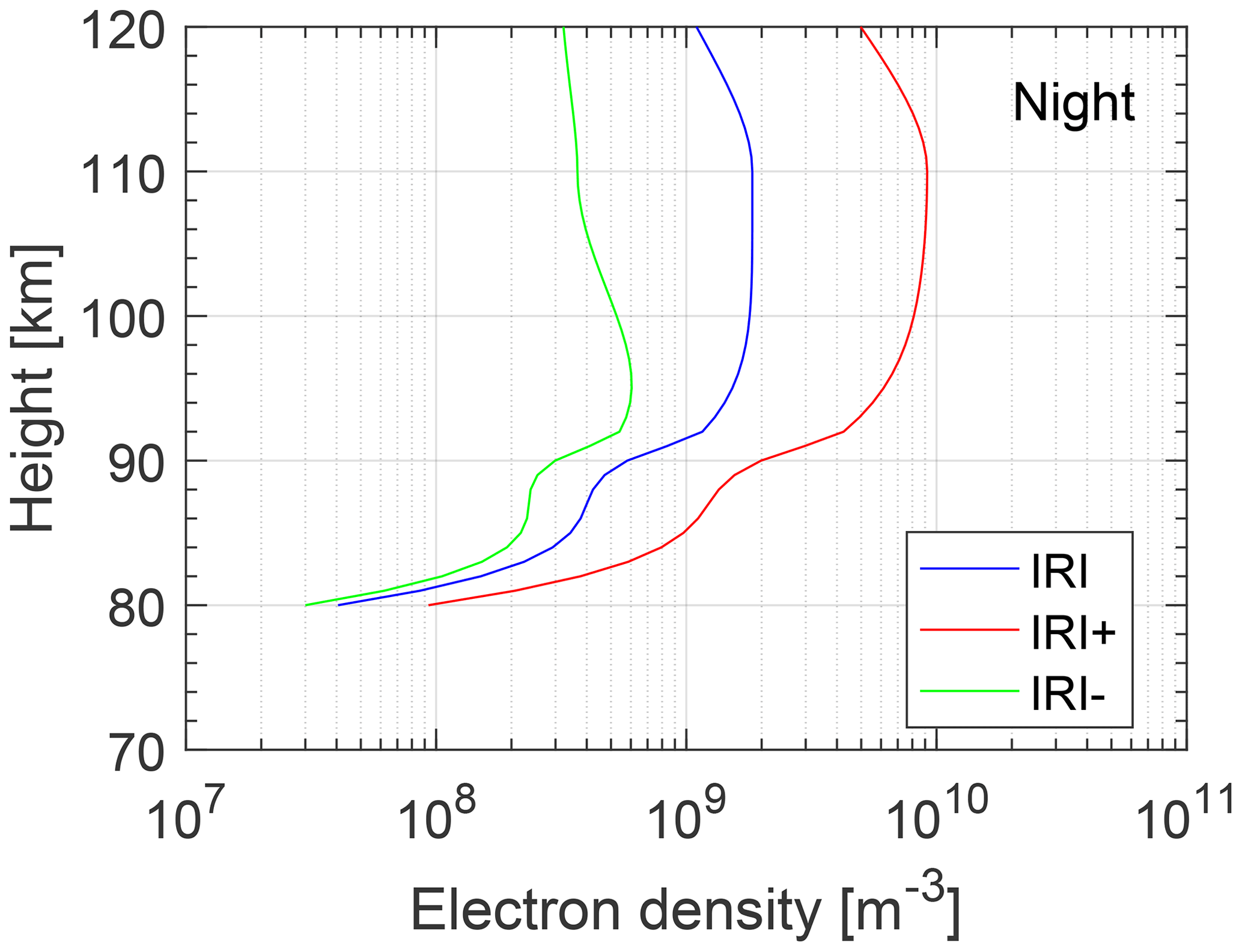
Figure 8The electron density profiles during nighttime. IRI represents the original electron density predicted by the IRI model; IRI+ represents the electron-density-added Gaussian shape perturbation; IRI- represents the electron-density-subtracted Gaussian shape perturbation.
We set a Gaussian shape perturbation at 110 with 20 km standard deviation in the ionosphere. The magnitude of the perturbation was set to a maximum of 1.3 and 4 times both the increase and decrease compared to the original electron density of nighttime (the average electron density above the NOV transmitter on 2–14 April 2010 at 22:00 LT calculated from the IRI-2016 model). The perturbation patterns are shown in Fig. 8 using 4 times the increase and decrease compared to the original electron density as an example. The electron collision frequency is modeled by the exponential-decay law described in Sect. 2.3. The geomagnetic-field intensity and inclination at the location of the NOV transmitter are calculated by the IGRF model.
The electric field only from the ground surface to 120 km has been calculated by the full-wave model because the electromagnetic wave at VLF band will propagate upward as the whistler mode. The group velocities of the upward-radiated whistler mode are almost parallel, and these waves form a narrow-collimated beam, which does not have much lateral spread. The direction of group velocities is determined by the refractive-index surface. The refractive-index surface of the upgoing whistler mode at 120 km is shown in Fig. 9. A ducted propagation is adopted at this L shell (Clilverd et al., 2008), and the VLF wave power is spread in accordance with the divergence of geomagnetic field lines with a linear reduction because of the mode conversion (Lehtinen and Inan, 2009; Shao et al., 2012). The abnormal region of TEC and SNR both that occurred in the southwestern region of the Yushu epicenter could demonstrate that the VLF radio wave propagated in a ducted mode.
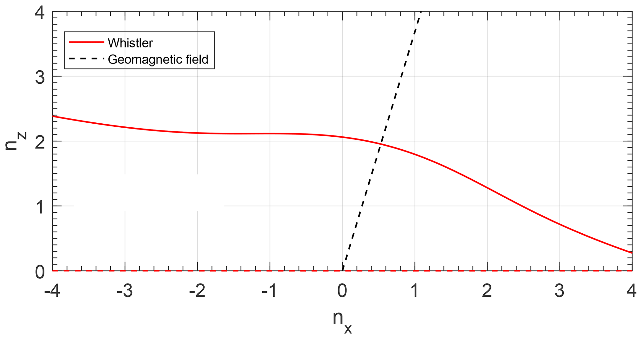
Figure 9The refractive-index surface at 120 km. Red line shows a slice of the refractive-index surface at ny=0 of the whistler mode, calculated for f=119 kHz at the altitude of h=120 km. Black dash line shows the direction of the geomagnetic field.
The simulated results of the electric field at 120 km height with a different electron density along the magnetic meridian plane within 1000 km area around the transmitter NOV with 11.9 kHz transmitting frequency are shown in Fig. 10. The simulated results are similar when the transmitting frequency is 12.6 and 14.9 kHz. It can be seen that the wave mode interference in the waveguide has been mapped into the ionosphere in the electric field (Lehtinen and Inan, 2009), and the electric field increases when the electron density decreases, and vice versa (Fig. 10a, c). Furthermore, the maximum value of the electric field varying with height is collected to study the influence of the electron disturbance. At nighttime, when i the variation of electron density is smaller, the variation of the electric field is also smaller (Fig. 10b, d). When the electron density increases by 4 times, the maximum electric field decreases about 2 dB at 120 km (see Fig. 10d). The variation is also 2 dB at DEMETER's altitude (660 km) because of the linear reductions (Lehtinen and Inan, 2009; Shao et al., 2012), which implies that the disturbed electric field decreased 20 % compared with the original electric field (Fig. 8b). In the short time interval of a few days before the earthquake, the background noise can be assumed to be stable, so the change in the electric field can reflect the change in SNR. It can be concluded that when the electron density increases by 4 times, the variation of SNR is 20 %. The simulated results illustrate that the variation of electron density in the lower ionosphere before an earthquake is one main factor of causing the abnormal variation of SNR. The more precise SNR variation needs more observation and simulation in the future.
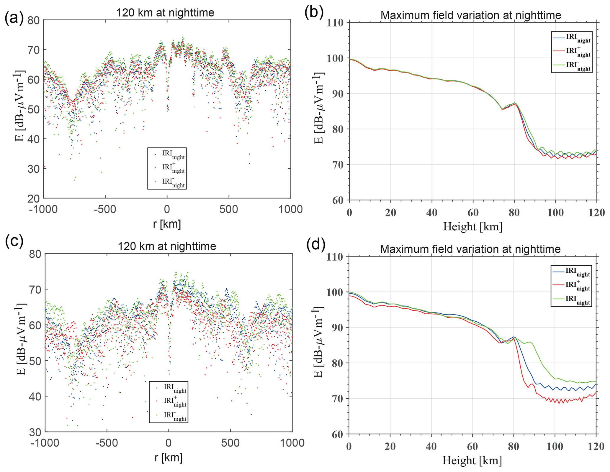
Figure 10The total electric field excited by the ground-based VLF transmitter NOV with a transmitting frequency of f=11.9 kHz and power of P=500 kW. The total electric field at the altitude of 120 km (a) and the maximum electric field varying with altitude (b) at nighttime when the Gaussian shape disturbance is set to 1.3 times compared with original electron density. The total electric field at the altitude of 120 km (c) and the maximum electric field varying with altitude (d) at nighttime when the Gaussian shape disturbance is set to 4 times compared with original electron density.
4.1 The possible mechanism on how the earthquake induces the disturbance in the lower ionosphere
Which coupling mechanism is effective to induce electron density anomalies in the D–E layer by earthquakes is still an open question. Molchanov et al. (2006) declared that the lower-ionospheric disturbance is caused by acoustic gravity waves triggered by earthquakes. At present, the coupling mechanism of the electric field proposed by Pulinets (2009) is widely accepted because it has been demonstrated by a series of models (Kuo et al., 2011; Namgaladze et al., 2013; Zhou et al., 2017) and observations (Gousheva et al., 2006, 2008; Li et al., 2017). As for the 2008 Wenchuan Ms 8.0 earthquake in China, Li et al. (2017) reported continuous observations about the anomalous electric field which lasted longer but weaker than the electric field induced by lightning during 1 month before the Wenchuan earthquake, which suggests that the abnormal electric field might be caused by the seismogenic activity of the Wenchuan earthquake. Xu et al. (2011) also found about 2 mV m−1 anomalous electric field in the F2 layer of the ionosphere before the Wenchuan earthquake. Gousheva et al. (2006, 2008) revealed a large number of anomalous electric fields before earthquakes using the INTERCOSMOS satellite. In addition, it is demonstrated that the anomalous electric field induced by an earthquake could change the electron density in the lower ionosphere by Kuo et al. (2011) and Zhou et al. (2017). Such as for the 2015 M 8.1 Nepal earthquake, the electron density variation was well explained by the ground electric-field coupling model established by Zhou et al. (2017).
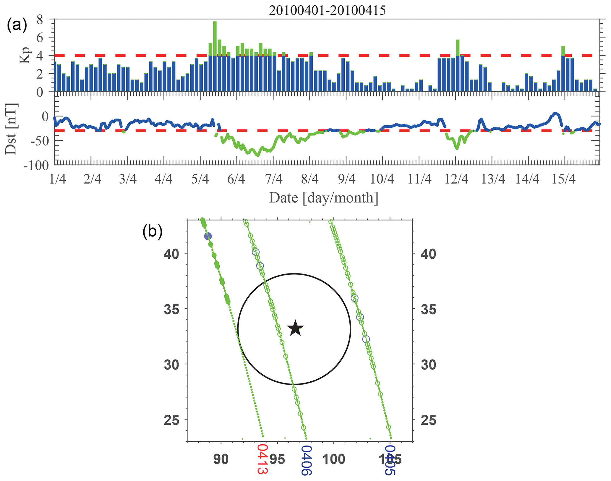
Figure 11The Kp and Dst index in April 2010 (a). The SNR distribution on 5 and 6 April with a geomagnetic storm and 13 April (1 d before the Yushu earthquake) (b). Please note that the date format of the heading is year month day, but the date format of the black text is day/month, and the date format of the red and blue text is month day.
4.2 The other factors may induce disturbance in the lower ionosphere
The lightning, geomagnetic storms, and other natural sources may induce disturbance in the lower ionosphere (Marshall et al., 2010; Maurya et al., 2016; Peter et al., 2006; Zigman et al., 2007). As known, the intensive TEC change occurs during geomagnetic storms, and the change in TEC is affected intensively during the main phase of the geomagnetic storm, gradually returning to normal accompanying the recovery phase. To avoid the effect of geomagnetic storms, the data which Kp > 3 and Dst nT were excluded in this research, and the TEC anomaly detected in Fig. 6 was seen 1 d after the recovery phase of the geomagnetic storm (Fig. 11a). Furthermore, the change pattern of TEC is totally different from the one caused by an earthquake because the TEC anomalies caused by a geomagnetic storm expand from high latitudes to mid latitudes due to thermospheric neutral winds, E × B convection, and so on (Pokhotelov et al., 2008). From Fig. 11b, we can see SNR on the whole orbit are large on 5–7 and 11 April during geomagnetic storms, especially at the higher latitudes. However, the SNR pattern on 13 April is totally different; SNRs on the orbit of 13 April only decrease in the abnormal TEC region. In sum, the TEC anomaly on 13 April should be unconcerned with the geomagnetic storm. A lightning flash is very rare in our research region (only four events from February 2010 to April 2010, which can be seen from the search result of https://lightning.nsstc.nasa.gov/nlisib/nlissearch.pl?coords=?579,18, last access: 27 August 2020), so the effect of lightning could be ignored in this study.
In this paper, the SNR of the electric field from a ground-based VLF transmitter observed by the DEMETER satellite was analyzed before and after the 2010 Ms 7.1 Yushu earthquake. The VLF signals from Russian VLF transmitters can be clearly observed at frequencies of 11.9, 12.6, and 14.9 kHz over the epicenter from the electric-field spectrum data. To determine whether the SNR variation is related to the Yushu earthquake, the data in quiet space weather conditions (Kp ≤ 3 and Dst ≥ −30 nT) have been selected during five satellite revisit periods before the earthquake and one revisit period after the earthquake. The result shows that SNR decreased during one revisit period before the Yushu earthquake in all cases. Our analysis of SNR variation also shows that SNR on 13 April is smaller than that on other days over the epicenter; the day-to-day variation of revisit orbit also demonstrates this point, and the decrease in SNR is the most intensive in the southwestern region when we divide the space over the epicenter of the earthquake into four regions. These results are consistent with the TEC anomalies in Fig. 6. In addition, we also analyzed the SNR changes over the epicenter in the same period from 2007 to 2010 as a background map and found that the SNR change trends of one revisit period before the earthquake relative to background time were contrary to those in 2010. The change trend of SNR decreased in 2010 but increased in background time in the first revisit period before the earthquake. The change trend of SNR is the same in other revisit periods both in 2010 and background time. In sum, it can be concluded that the SNR over the epicenter of the Yushu earthquake decreases abnormally in one satellite revisit period before the earthquake, especially in the southwestern region of the earthquake, which is consistent with the observed TEC anomaly before the earthquake. The decrease in SNR before the Yushu earthquake may be due to the enhancement of electron density.
The electron density in the lower ionosphere may change abnormally before an earthquake through some coupling mechanisms. The full-wave simulation result on NOV transmitter, which is the nearest transmitter next to the Yushu earthquake, indicates that the electric field at the altitude of a satellite will change when we add a disturbance of electron density in the lower ionosphere. That is to say that the SNR of the electric field will also change when the background noise is considered to be invariable a few days before the earthquake. The simulated results show SNR does not always decrease before an earthquake like some previous reports show (He et al., 2009; Molchanov et al., 2006; Yao et al., 2013), which depends on the change in electron density. The SNR of the electric field will decrease with the increase in electron density in the lower ionosphere; SNR will increase with the decrease in electron density in the lower ionosphere. It can be concluded that the variation of electron density before earthquakes may be one important factor influencing the variation of SNR.
We will continually explore the law of SNR change and verify the mechanism we proposed with more seismic events by utilizing the newly launched LEO electromagnetic satellite (China Seismo-Electromagnetic Satellite) (Shen et al., 2018; Zhao et al., 2019) in upcoming work.
The DEMETER satellite data were provided by the DEMETER scientific mission center (http://demeter.cnrs-orleans.fr, last access: 27 August 2020). The GPS–TEC data were provided by CODE (Center for Orbit Determination in Europe) and can be downloaded from ftp://cddis.gsfc.nasa.gov/pub/gps/products/ionex (last access: 27 August 2020). The COSMIC, Dst, and Kp data can be obtained from https://cdaac-www.cosmic.ucar.edu/cdaac/cgi_bin/fileFormats.cgi?type=ionPrf (last access: 27 August 2020, University Corporation for Atmospheric Research, 2020), http://wdc.kugi.kyoto-u.ac.jp/dst_final/index.html (last access: 27 August 2020, World Data Center, 2020), and ftp://ftp.gfz-potsdam.de/pub/home/obs/kp-ap/wdc/yearly/ (last access: 27 August 2020, GFZ German Research Centre for Geosciences, 2020), respectively.
SZ conceptualized the project, performed the formal analysis and investigation, supervised the project, created the visualizations, and wrote the original draft of the paper. SZ, RZ, and XS conceptualized the methodology and secured the project's resources. SZ, RZ, CZ, and XS reviewed and edited the paper.
The authors declare that they have no conflict of interest.
This article is part of the special issue “Satellite observations for space weather and geo-hazard”. It is not associated with a conference.
This paper benefited from constructive review comments by two anonymous reviewers and the editor. Thanks for their advice and help.
This research has been supported by the National Science Foundation of China (grant nos. 41704156, 41574139, and 41874174), the National Key R&D Program of China (grant no. 2018YFC1503501), the Special Fund of the Institute of Earthquake Forecasting, China Earthquake Administration (grant nos. 2015IES010103 and 2018CSES0203), and the APSCO Earthquake Research Project Phase II.
This paper was edited by Mirko Piersanti and reviewed by two anonymous referees.
Bilitza, D., Altadill, D., Truhlik, V., Shubin, V., Galkin, I., Reinisch, B., and Huang, X.: International Reference Ionosphere 2016: From ionospheric climate to real-time weather predictions, Space Weather, 15, 418–429, 2017.
Budden, K.: The Propagation Of Radio Waves: The Theory Of Radio Waves Of Low Power In The Ionosphere And Magnetosphere, Cambridge University Press, Cambridge, United Kingdom, 669 pp., 1985.
Clilverd, M. A., Rodger, C. J., Gamble, R., Meredith, N. P., Parrot, M., Berthelier, J. J., and Thomson, N. R.: Ground-based transmitter signals observed from space: Ducted or nonducted?, J. Geophys. Res.-Atmos., 113, A04211, https://doi.org/10.1029/2007JA012602, 2008.
Cohen, M. B. and Inan, U. S.: Terrestrial VLF transmitter injection into the magnetosphere, J. Geophys. Res.-Space, 117, https://doi.org/10.1029/2012JA017992, 2012.
Dobrovolsky, I. P., Zubkov, S. I., and Miachkin, V. I.: Estimation of the size of earthquake preparation zones, Pure Appl. Geophys., 117, 1025–1044, 1979.
Finlay, C. C., Maus, S., Beggan, C. D., Bondar, T. N., Chambodut, A., Chernova, T. A., Chulliat, A., Golovkov, V. P., Hamilton, B., Hamoudi, M., Holme, R., Hulot, G., Kuang, W., Langlais, B., Lesur, V., Lowes, F. J., Luhr, H., Macmillan, S., Mandea, M., McLean, S., Manoj, C., Menvielle, M., Michaelis, I., N., O., Rauberg, J., Rother, M., Sabaka, T. J., Tangborn, A., L., T.-C., Thebault, E., Thomson, A. W. P., Wardinski, I., Wei, Z., and Zvereva, T. I.: International Geomagnetic Reference Field: the eleventh generation, Geophys. J. Int., 183, 1216–1230, 2010.
GFZ German Research Centre for Geosciences: Kp index FTP, available at: ftp://ftp.gfz-potsdam.de/pub/home/obs/kp-ap/wdc/yearly/, last access: 27 August 2020.
Gousheva, M., Glavcheva, R., Danov, D., Angelov, P., Hristov, P., Kirov, B., and Georgieva, K.: Satellite monitoring of anomalous effects in the ionosphere probably related to strong earthquakes, Adv. Space Res., 37, 660–665, 2006.
Gousheva, M., Glavcheva, R., Danov, D., Hristov, P., Kirov, B. B., and Georgieva, K.: Electric field and ion density anomalies in the mid latitude ionosphere: Possible connection with earthquakes?, Adv. Space Res., 42, 206–212, 2008.
Hayakawa, M.: VLF/LF Radio Sounding of Ionospheric Perturbations Associated with Earthquakes, Sensors, 7, 1141–1158, 2007.
He, Y., Yang, D., Chen, H., Qian, J., Zhu, R., and Parrot, M.: SNR changes of VLF radio signals detected onboard the DEMETER satellite and their possible relationship to the Wenchuan earthquake, Science in China Series D-Earth Sciences, 39, 403–412, 2009,
Inan, U. S., Golkowski, M., Casey, M. K., Moore, R. C., Peter, W. B., Kulkarni, P., Kossey, P., Kennedy, E., Meth, S., and Smit, P.: Subionospheric VLF observations of transmitter-induced precipitation of inner radiation belt electrons, Geophys. Res. Lett., 34, L02106, https://doi.org/10.1029/2006GL028494, 2007.
Inan, U. S. and Helliwell, R. A.: DE-1 observations of VLF transmitter signals and wave-particle interactions in the magnetosphere, Geophys. Res. Lett., 9, 917–920, 1982.
Kong, J., Yao, Y., Zhou, C., Liu, Y., Zhai, C., Wang, Z., and Liu, L.: Tridimensional reconstruction of the Co-Seismic Ionospheric Disturbance around the time of 2015 Nepal earthquake, J. Geodesy, 92, 1255–1266, 2018.
Kuo, C. L., Huba, J. D., Joyce, G., and Lee, L. C.: Ionosphere plasma bubbles and density variations induced by pre-earthquake rock currents and associated surface charges, J. Geophys. Res.-Space, 116, https://doi.org/10.1029/2011JA016628, 2011.
Lehtinen, N. G. and Inan, U. S.: Radiation of ELF/VLF waves by harmonically varying currents into a stratified ionosphere with application to radiation by a modulated electrojet, J. Geophys. Res., 113, https://doi.org/10.1029/2007JA012911, 2008.
Lehtinen, N. G. and Inan, U. S.: Full-wave modeling of transionospheric propagation of VLF waves, Geophys. Res. Lett., 36, https://doi.org/10.1029/2008GL036535, 2009.
Li, Y., Zhang, L., Zhang, K., and Jin, X.: Research on the Atmospheric Electric Field Abnormality near the Ground Surface before 5, 12 Wenchuan Earthquake, Plateau and Mountain Meteorology Research, 37, 49–53, 2017.
Liao, L., Zhao, S., and Zhang, X.: Advances in the study of transionospheric propagation of VLF waves, Chinese Journal of Space Science, 37, 277–283, 2017.
Liu, J. Y., Chen, Y. I., Chen, C. H., Liu, C. Y., Chen, C. Y., Nishihashi, M., Li, J. Z., Xia, Y. Q., Oyama, K. I., Hattori, K., and Lin, C. H.: Seismoionospheric GPS total electron content anomalies observed before the 12 May 2008 Mw7.9 Wenchuan earthquake, J. Geophys. Res.-Space, 114, https://doi.org/10.1029/2008JA013698, 2009.
Liu, J. Y., Chen, Y. I., Chuo, Y. J., and Tsai, H. F.: Variations of ionospheric total electron content during the Chi-Chi earthquake, Geophys. Res. Lett., 28, 1383–1386, 2001.
Liu, J. Y., Tsai, Y. B., Chen, S. W., Lee, C. P., Chen, Y. C., Yen, H. Y., Chang, W. Y., and Liu, C.: Giant ionospheric disturbances excited by the M9.3 Sumatra earthquake of 26 December 2004, Geophys. Res. Lett., 33, https://doi.org/10.1029/2005GL023963, 2006.
Marshall, R. A., Inan, U. S., and Glukhov, V. S.: Elves and associated electron density changes due to cloud-to-ground and in-cloud lightning discharges, J. Geophys. Res.-Space, 115, https://doi.org/10.1029/2009JA014469, 2010.
Maurya, A. K., Venkatesham, K., Tiwari, P., Vijaykumar, K., Singh, R., Singh, A. K., and Ramesh, D. S.: The 25 April 2015 Nepal Earthquake: Investigation of precursor in VLF subionospheric signal, J. Geophys. Res.-Space 121, 10403–10416, 2016.
Molchanov, O., Rozhnoi, A., Solovieva, M., Akentieva, O., Berthelier, J. J., Parrot, M., Lefeuvre, F., Biagi, P. F., Castellana, L., and Hayakawa, M.: Global diagnostics of the ionospheric perturbations related to the seismic activity using the VLF radio signals collected on the DEMETER satellite, Nat. Hazards Earth Syst. Sci., 6, 745–753, https://doi.org/10.5194/nhess-6-745-2006, 2006.
Namgaladze, A. A., Zolotov, O. V., and Prokhorov, B. E.: Numerical Simulation of the Variations in the Total Electron Content of the Ionosphere Observed before the Haiti Earthquake of January 12, 2010, Geomagn. Aeronomy, 53, 522–528, 2013.
Parrot, M., Benoist, D., Berthelier, J. J., Błęcki, J., Chapuis, Y., Colin, F., Elie, F., Fergeau, P., Lagoutte, D., and Lefeuvre, F.: The magnetic field experiment IMSC and its data processing onboard DEMETER: Scientific objectives, description and first results, Planet. Space Sci., 54, 441–455, 2006.
Parrot, M., Sauvaud, J., Berthelier, J., and Lebreton, J.: First in-situ observations of strong ionospheric perturbations generated by a powerful VLF ground-based transmitter, Geophys. Res. Lett., 34, https://doi.org/10.1029/2007GL029368, 2007.
Peter, W. B., Chevalier, M. W., and Inan, U. S.: Perturbations of midlatitude subionospheric VLF signals associated with lower ionospheric disturbances during major geomagnetic storms, J. Geophys. Res.-Space, 111, https://doi.org/10.1029/2005JA011346, 2006.
Píša, D., Němec, F., Santolík, O., Parrot, M., and Rycroft, M.: Additional attenuation of natural VLF electromagnetic waves observed by the DEMETER spacecraft resulting from preseismic activity, J. Geophys. Res.-Space, 118, 5286–5295, 2013.
Pokhotelov, D., Mitchell, C. N., Spencer, P. S. J., Hairston, M. R., and Heelis, R. A.: Ionospheric storm time dynamics as seen by GPS tomography and in situ spacecraft observations, J. Geophys. Res.-Space, 113, https://doi.org/10.1029/2008JA013109, 2008.
Pulinets, S. A.: Physical mechanism of the vertical electric field generation over active tectonic faults, Adv. Space Res., 44, 767–773, 2009.
Pulinets, S. A., Boyarchuk, K. A., Hegai, V. V., Kim, V. P., and Lomonosov, A. M.: Quasielectrostatic model of atmosphere-thermosphere-ionosphere coupling, Adv. Space Res., 26, 1209–1218, 2000.
Shao, X., Eliasson, B., Sharma, A., Milikh, G., and Papadopoulos, K.: Attenuation of whistler waves through conversion to lower hybrid waves in the low-altitude ionosphere, J. Geophys. Res.-Space, 117, https://doi.org/10.1029/2011JA017339, 2012.
Shen, X., Zhima, Z., Zhao, S., Qian, G., Ye, Q., and Ruzhin, Y.: VLF radio wave anomalies associated with the 2010 Ms 7.1 Yushu earthquake, Adv. Space Res., 59, 2636–2644, 2017.
Shen, X. H., Zhang, X. M., Yuan, S. G., Wang, L. W., Cao, J. B., Huang, J. P., Zhu, X. H., Piergiorgio, P., and Dai, J. P.: The state-of-the-art of the China Seismo-Electromagnetic Satellite mission, Sci China Technol. Sc., 61, 634–642, 2018.
Stangl, G., Boudjada, M. Y., Biagi, P. F., Krauss, S., Maier, A., Schwingenschuh, K., Al-Haddad, E., Parrot, M., and Voller, W.: Investigation of TEC and VLF space measurements associated to L'Aquila (Italy) earthquakes, Nat. Hazards Earth Syst. Sci., 11, 1019–1024, https://doi.org/10.5194/nhess-11-1019-2011, 2011.
Starks, M. J., Quinn, R. A., Ginet, G. P., Albert, J. M., Sales, G. S., Reinisch, B. W., and Song, P.: Illumination of the plasmasphere by terrestrial very low frequency transmitters: Model validation, J. Geophys. Res.-Space, 113, https://doi.org/10.1029/2008JA013112, 2008.
Tao, X., Bortnik, J., and Friedrich, M.: Variance of transionospheric VLF wave power absorption, J. Geophys. Res.-Space, 115, https://doi.org/10.1029/2009JA015115, 2010.
University Corporation for Atmospheric Research: COSMIC Data Analysis and Archive Center Home Page, available at: https://cdaac-www.cosmic.ucar.edu/cdaac/cgi_bin/fileFormats.cgi?type=ionPrf, last access: 27 August 2020.
World Data Center: Geomagnetic Equatorial Dst index Home Page, available at: http://wdc.kugi.kyoto-u.ac.jp/dst_final/index.html, last access: 27 August 2020.
Xu, T., Hu, Y. L., Wu, J. A., Wu, Z. S., Li, C. B., Xu, Z. W., and Suo, Y. C.: Anomalous enhancement of electric field derived from ionosonde data before the great Wenchuan earthquake, Adv. Space Res., 47, 1001–1005, 2011.
Yao, L., Chen, H., and He, Y.: The signal to noise ratio disturbance of ionospheric VLF radio signal before the 2010 Yushu Ms7.1 earthquake, Acta Seismol. Sin., 35, 390–399, 2013.
Yeh, K. C. and Liu, C. H.: Theory of Ionospheric Waves, Academic Press, New York, 464 pp., 1972.
Zhao, B. Q., Wang, M., Yu, T., Wan, W. X., Lei, J. H., Liu, L. B., and Ning, B. Q.: Is an unusual large enhancement of ionospheric electron density linked with the 2008 great Wenchuan earthquake?, J. Geophys. Res.-Space, 113, https://doi.org/10.1029/2008JA013613, 2008.
Zhao, S., Liao, L., and Zhang, X.: Trans-ionospheric VLF wave power absorption of terrestrial VLF signal, Chinese Journal of Geophysics, 60, 3004–3014, 2017.
Zhao, S., Zhang, X., Zhao, Z., Shen, X., and Chen, Z.: Temporal variations of electromagnetic responses in the ionosphere excited by the NWC communication station, Chinese Journal of Geophysics-Chinese Edition, 58, 2263–2273, 2015.
Zhao, S., Zhou, C., Shen, X., and Zhima, Z.: Investigation of VLF transmitter signals in the ionosphere by ZH-1 observations and full-wave simulation, J. Geophys. Res.-Space, 124, 4697–4709, 2019.
Zhou, C., Liu, Y., Zhao, S. F., Liu, J., Zhang, X. M., Huang, J. P., Shen, X. H., Ni, B. B., and Zhao, Z. Y.: An electric field penetration model for seismo-ionospheric research, Adv. Space Res., 60, 2217–2232, 2017.
Zigman, V., Grubor, D., and Sulic, D.: D-region electron density evaluated from VLF amplitude time delay during X-ray solar flares, J. Atmos. Sol.-Terr. Phy., 69, 775–792, 2007.