the Creative Commons Attribution 4.0 License.
the Creative Commons Attribution 4.0 License.
 | 08 Jul 2020
Nighttime O(1D) distributions in the mesopause region derived from SABER data
Mikhail Yu. Kulikov
Mikhail V. Belikovich
In this study, the new source of O(1D) in the mesopause region due to the process OH) is applied to SABER data to estimate the nighttime O(1D) distributions for the years 2003–2005. It is found that O(1D) evolutions in these years are very similar to each other. Depending on the month, monthly averaged O(1D) distributions show two to four maxima with values up to 340 cm−3 which are localized in height (at ∼92–96 km) and latitude (at ∼20–40 and ∼60–80∘ S, N). Annually averaged distributions in 2003–2005 have one weak maximum at ∼93 km and ∼65∘ S with values of 150–160 cm−3 and three pronounced maxima (with values up to 230 cm−3) at ∼95 km and ∼35∘ S, at ∼94 km and ∼40∘ N and at ∼93 km and ∼65–75∘ N, correspondingly. In general, there is slightly more O(1D) in the Northern Hemisphere than in the Southern Hemisphere. The obtained results are a useful data set for subsequent estimation of nighttime O(1D) influence on the chemistry of the mesopause region.
- Article
(6897 KB) - Full-text XML
- BibTeX
- EndNote


Daytime O(1D) is considered to be one of the important chemical minor species of the stratosphere, mesosphere and thermosphere, as it plays a significant role in the chemistry and the radiative and thermal balance of this region (Brasseur and Solomon, 2005). First of all, formed by photolysis of O2 and O3, O(1D) is a mediator involved in the transformation of absorbed solar radiation energy into the heating of this region and, in particular, excitation of N2(ν) and CO2(ν) (Harris and Adams, 1983; Panka et al., 2017). Also, O(1D) atoms participate in the reactions of destruction of long-lived greenhouse gases (Baasandorj et al., 2012), CH4 oxidation, and HOx and NOx production. For example:
Moreover, the red line emission from O(1D) atoms is one of the most important airglow phenomena which are used as a diagnostic of the ionosphere, for example, to monitor the electron density and neutral winds in the F region (Shepherd et al., 2019). Therefore, many papers and experimental campaigns are devoted to measurements of features of O3 photolysis to O(1D) (Taniguchi et al., 2003; Hofzumahaus et al., 2004).
Until recently, it was believed that the above-mentioned processes stopped at night as a continuous source of O(1D) is absent, while the lifetime of the component is extremely short (less than 1 s). In principle, O(1D) can be generated in sprite halos but for a short duration of 1 ms (Hiraki et al., 2004). Recently, Sharma et al. (2015) and Kalogerakis et al. (2016), based on laboratory experiments, proposed that O(1D) could be produced in the mesopause region via the process OH(ν≥5) + O(3P) → OH() + O(1D), which is multiquantum quenching of high excited states of OH by collisions with atomic oxygen in the ground state.
Last year, Kalogerakis (2019) showed that a new model of O2 A-band that takes this process into account describes well (qualitatively and quantitatively) the results of early nighttime rocket measurements of volume emission rate profiles of this airglow. Thus, he proved that the process OH(ν≥5) + O(3P) → OH() + O(1D) really took place in the nighttime mesopause, and the produced O(1D) distributions can be evaluated from available data.
In this study, the new source of O(1D) in the mesopause region is applied to SABER data to estimate the O(1D) nighttime distributions for the years 2003–2005.
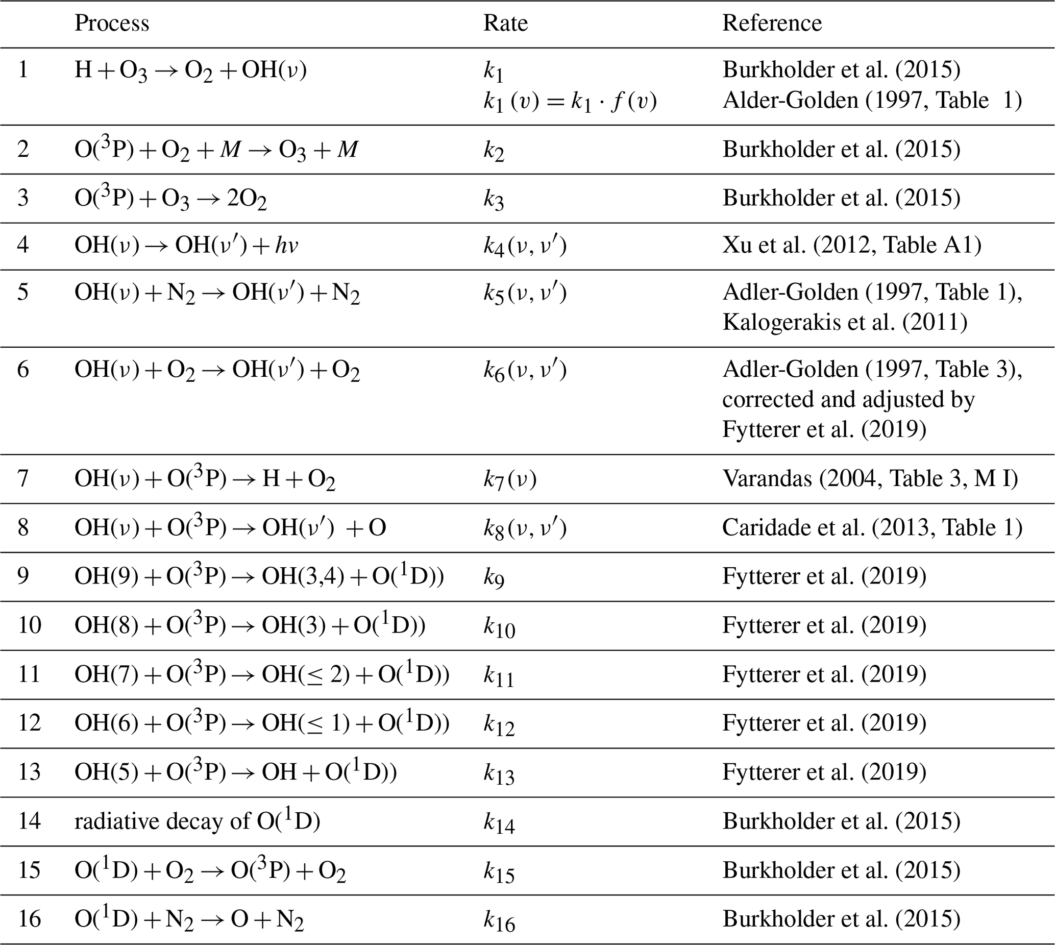
Table 2List of systematic uncertainties of measured data and rate constants and corresponding uncertainties in derived O(1D) local concentration.
All processes used for O(1D) determination are summarized in Table 1. Here, we apply the new OH(v) model of Fytterer et al. (2019). Their “best-fit model” includes all commonly used production and loss processes of OH(v) (see Table 1), but some parameters of the model, in particular, branching ratios of quenching OH(v) + O2 and rate coefficients of OH(ν≥5) + O(3P) → OH() + O(1D), were adjusted with the use of volume emission rate profiles at four different wavelengths measured by SABER and SCIAMACHY.
Due to low values of chemical lifetimes (less than 1 s), O(1D) can be considered in chemical equilibrium:
Thus, to calculate the local value of O(1D), we should specify the local concentrations of OH(v=5–9) and O(3P). The mentioned model lets us derive the OH(v) concentrations as the functions of the OH(v) source due to the reaction H + O3 (), air concentration (M), temperature (T), and O(3P) concentration:
To determine O(3P) and POH, we use the known (e.g., Mlynczak et al., 2013, 2018) approach for O(3P) derivation from the simultaneous SABER measurements of total volume emission rate of (9–7) and (8–6) OH transitions (VER2 µm), O3 (9.6 µm), and temperature (T). The approach employs the chemical equilibrium condition for nighttime ozone. As a result, it is done with the use of the following system of equations:
Thus, we derive the local values of O(3P), POH, and OH(v=5–9) from SABER data with the use of Eqs. (2)–(3) and apply sets of data (T, M, OH(v=5–9), and O(3P)) to retrieve the local concentrations of O(1D) with the use of Eq. (1).
The systematic uncertainty of retrieved data is defined by uncertainties in VER2 µm, O3, T measurements, and the rates of chemical and physical processes included in the OH(v) model. We reproduced the analysis presented in Fytterer et al. (2019) (see Sect. 3.4) and took into account the uncertainties of measured data and rate constants which are shown in Table 2. The third column of the table demonstrates the uncertainties' individual impact at derived O(1D) local concentration. It can be noted that the most critical for O(1D) are the uncertainties in T, rates of Reactions (2)–(3), Einstein coefficients for the v=8–9 states, and VER2 µm. The total systematic O(1D) uncertainty was obtained by calculating the root-sum square of all individual uncertainties. It was found to vary in the range of (37%–52%) depending on the pressure level. Due to averaging, the random error of data presented below is negligible.
We use version 2.0 of the SABER data product (Level2A) for the simultaneously measured VER2 µm, O3, and T profiles within the 0.01–0.0001 hPa pressure (p) interval (approximately 80–105 km in 2003–2005). We take only nighttime data when the solar zenith angle is greater than 95∘. The range of latitudes covered by the satellite trajectory in a month was divided into 20 bins of ∼(5.5–8)∘ each; 1500–3000 single profiles of O(1D) concentration fall into 1 bin during a month of SABER observations. For each bin we calculate monthly averaged zonal mean <O(1D)> distributions (hereafter, the angle brackets are used to denote timely and spatially averaged values). For annually averaged distributions, we use 40 bins of each.
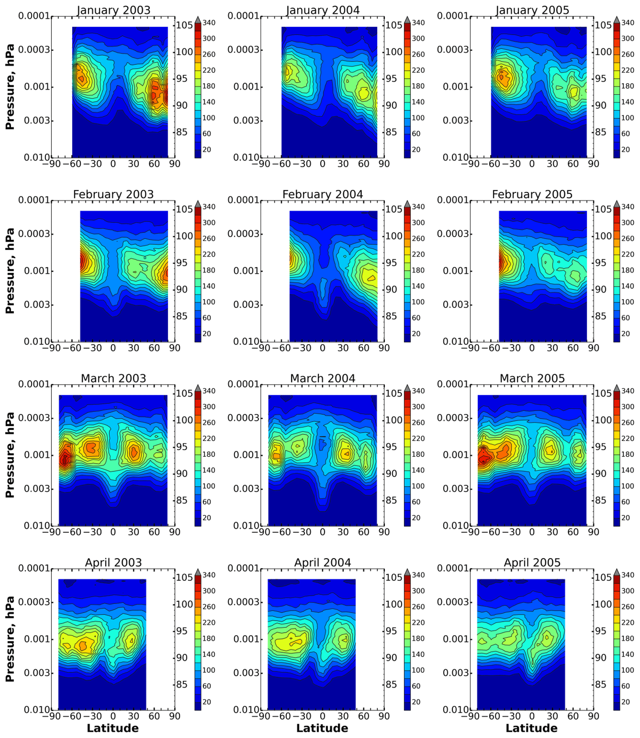
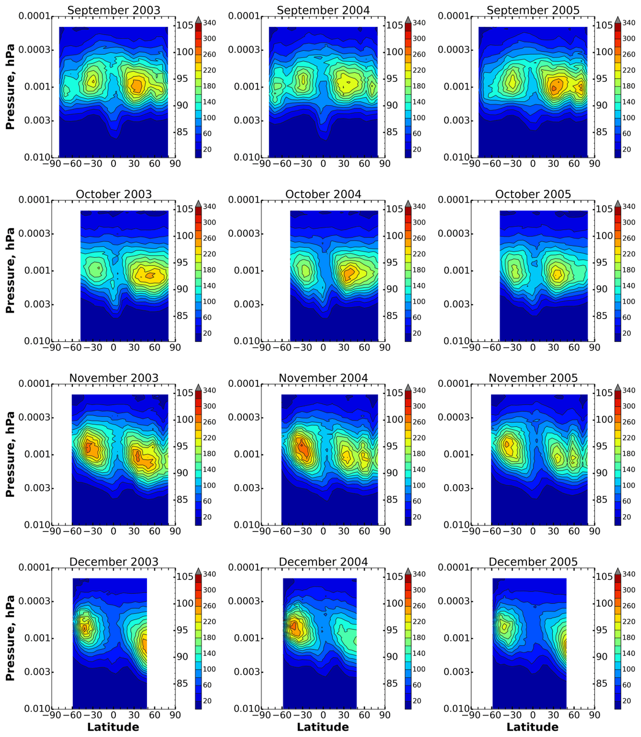
Monthly averaged distributions in corresponding months of 2003–2005 are shown in Figs. 1–3. Let us analyze the presented data using the distributions in 2003 as an example. Depending on the range of latitudes covered by the satellite trajectory in a specified month, the figures show two to four maxima which are localized in height (at ∼92–96 km) and latitude (at ∼20–40 and ∼60–80∘ S, N). The values of the maxima can reach up to 300 cm−3 and more in both hemispheres and different months, for example, in January–March and in May–August. Nevertheless, the annual cycle of southern O(1D) demonstrates certain differences from the northern one; i.e., many features of in the Southern Hemisphere are not repeated in the Northern Hemisphere, with a shift of 6 months. In particular, the distributions in January–February show two pronounced maxima with close values (up to 300 cm−3): the first one is at ∼95 km and ∼50–60∘ S, the second one at ∼93 km and ∼60–80∘ N. Half a year later (in July–August), we can see one to two weak maxima in the Southern Hemisphere and a strongly pronounced maximum at ∼95 km and ∼40–50∘ N. A similar pattern can be noticed when comparing the distributions in June and December. The satellite trajectory in March and September allows us to observe simultaneously four maxima. Note that the southern high-latitudinal maximum (up to 340 cm−3) in March does not correspond to the relatively weak northern high-latitudinal maximum in September.
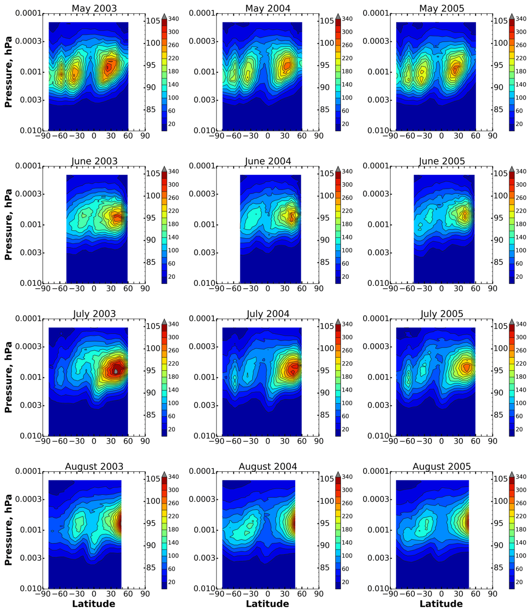
The evolutions in 2004–2005 are very similar to 2003. Nevertheless, one can see some differences. First of all, in January–February 2004, there is a pronounced particularity above 60∘ N below 90 km which does not appear in 2003 and 2005. Kulikov et al. (2019) found similar features in the latitude dependence of the nighttime ozone chemical equilibrium boundary (the lower boundary of the altitudinal–latitudinal region where this equilibrium is satisfied; Belikovich et al., 2018; Kulikov et al., 2018) in January–March 2004 above 60∘ N and connected it with abnormal dynamics of the stratospheric polar vortex during the 2003–2004 Arctic winter. There are also additional features which are present in a specific year but absent in the other 2 years. In particular, the northern high-latitudinal maximum in January–February 2003 is remarkably higher (by the value) than the ones in January–February 2004–2005. The southern high-latitudinal maximum (up to 340 cm−3) in March 2003 corresponds to the same maximum in March 2005, but both maxima are remarkably higher than the one in March 2004. The reverse (relative to December 2003 and 2005) ratio can be observed for the values of southern and northern maxima in December 2004.
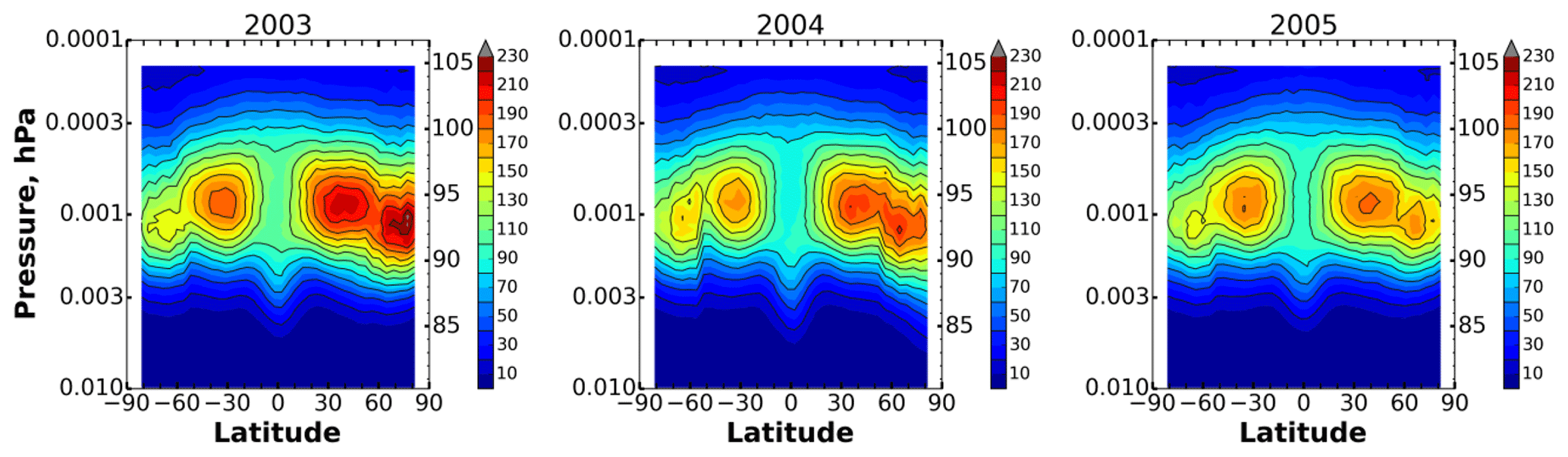
Annually averaged distributions in 2003–2005 are shown in Fig. 4. One can see one weak maximum at ∼93 km and ∼65∘ S, with values of 150–160 cm−3 and three pronounced maxima (with values up to 230 cm−3) at ∼95 km and ∼35∘ S, at ∼94 km and ∼40∘ N, and at ∼93 km and ∼65–75∘ N. In general, there is slightly more O(1D) in the Northern Hemisphere than in the Southern Hemisphere.
According to various early papers (Nicolet, 1959; Ghosh and Gupta, 1970; Shimazaki and Laird, 1970; Harris and Adams, 1983), daytime O(1D) concentrations at 90–100 km varied in the range of (102–103) cm−3. Brasseur and Solomon (2005) published the table (see Table A.6.2.c) where daytime O(1D) changed from 70 cm−3 at 90 km to 140 cm−3 at 100 km. The presented results show that monthly and annual mean nighttime O(1D) concentrations at these altitudes can reach 300 and 200 cm−3, respectively. Thus, nighttime concentrations of O(1D) are comparable with daytime concentrations of this component and, in principle, can impact noticeably the chemistry and thermal balance of the mesopause region. The analysis of this impact should be carried out with the use of a global 3D chemical transport model of the mesosphere–lower thermosphere. Additionally, it may indicate measurable characteristics of this region that could indirectly confirm the results obtained in this article. In principle, direct evidence of O(1D) layer existence in the nighttime mesopause can be established by in situ measurements of O(1D) airglow at 630 nm, which can be carried out, for example, as a part of a future WADIS rocket sounding mission (Strelnikov et al., 2019; Grygalashvyly et al., 2019). More detailed analysis is out of this short article's scope.
The SABER data used in this study can be downloaded from ftp://saber.gats-inc.com/Version2_0/Level2A/. The presented data can be downloaded from https://ipfran.ru/files/10564/article_2020_o1d_data.nc (last access: 2 July 2020).
Both authors contributed equally to this paper.
The authors declare that they have no conflict of interest.
The authors are grateful to the SABER team for data availability.
The work was carried out at the expense of state assignment no. 0729-2020-0037.
This paper was edited by Gunter Stober and reviewed by one anonymous referee.
Adler-Golden, S.: Kinetic parameters for OH nightglow modeling consistent with recent laboratory measurements, J. Geophys. Res., 102, 19969–19976, https://doi.org/10.1029/97JA01622, 1997.
Baasandorj, M., Hall, B. D., and Burkholder, J. B.: Rate coefficients for the reaction of O(1D) with the atmospherically long-lived greenhouse gases NF3, SF5CF3, CHF3, C2F6, c-C4F8, n-C5F12, and n-C6F14, Atmos. Chem. Phys., 12, 11753–11764, https://doi.org/10.5194/acp-12-11753-2012, 2012.
Belikovich, M. V., Kulikov, M. Y., Grygalashvyly, M., Sonnemann, G. R., Ermakova, T. S., Nechaev, A. A., and Feigin, A. M.: Ozone chemical equilibrium in the extended mesopause under the nighttime conditions, Adv. Space Res., 61, 426–432, https://doi.org/10.1016/j.asr.2017.10.010, 2018.
Brasseur, G. P. and Solomon, S.: Aeronomy of the middle atmosphere: Chemistry and physics of the stratosphere and mesosphere (3 Edn.), Dordrecht, Netherlands: Springer Science and Business Media, 644 pp., 2005.
Burkholder, J. B., Sander, S. P., Abbatt, J., Barker, J. R., Huie, R. E., Kolb, C. E., Kurylo, M. J., Orkin, V. L., Wilmouth, D. M., and Wine, P. H.: Chemical kinetics and photochemical data for use in atmospheric studies, evaluation no. 18, JPL Publication 15–10, Pasadena, CA: Jet Propulsion Laboratory, available at: http://jpldataeval.jpl.nasa.gov, (last access: 2 July 2020), 2015.
Caridade, P. J. S. B., Horta, J.-Z. J., and Varandas, A. J. C.: Implications of the O + OH reaction in hydroxyl nightglow modeling, Atmos. Chem. Phys., 13, 1–13, https://doi.org/10.5194/acp-13-1-2013, 2013.
Fytterer, T., von Savigny, C., Mlynczak, M., and Sinnhuber, M.: Model results of OH airglow considering four different wavelength regions to derive night-time atomic oxygen and atomic hydrogen in the mesopause region, Atmos. Chem. Phys., 19, 1835–1851, https://doi.org/10.5194/acp-19-1835-2019, 2019.
García-Comas, M., López-Puertas, M., Marshall, B. T., Wintersteiner, P. P., Funke, B., Bermejo-Pantaleón, D., Mertens, C. J., Remsberg, E. E., Gordley, L. L., Mlynczak, M. G., and Russell III, J. M.: Errors in Sounding of the Atmosphere using Broadband Emission Radiometry (SABER) kinetic temperature caused by non-local-thermodynamic equilibrium model parameters, J. Geophys. Res., 113, D24106, https://doi.org/10.1029/2008JD010105, 2008.
Ghosh, S. N. and Gupta, S. K.: Altitude distributions of and radiations from certain oxygen and nitrogen metastable constituents, J. Geomagn. Geoelectr., 22, 329–339, 1970.
Grygalashvyly, M., Eberhart, M., Hedin, J., Strelnikov, B., Lübken, F.-J., Rapp, M., Löhle, S., Fasoulas, S., Khaplanov, M., Gumbel, J., and Vorobeva, E.: Atmospheric band fitting coefficients derived from a self-consistent rocket-borne experiment, Atmos. Chem. Phys., 19, 1207–1220, https://doi.org/10.5194/acp-19-1207-2019, 2019.
Harris, R. D. and Adams, G. W.: Where does the O(1D) energy go?, J. Geophys. Res., 88, 4918–4928, https://doi.org/10.1029/JA088iA06p04918, 1983.
Hiraki, Y., Tong, L., Fukunishi, H., Nanbu, K., Kasai, Y., and Ichimura, A.: Generation of metastable oxygen atom O(1D) in sprite halos, Geophys. Res. Lett., 31, L14105, https://doi.org/10.1029/2004GL020048, 2004.
Hofzumahaus, A., Lefer, B. L., Monks, P. S., Hall, S. R., Kylling, A., Mayer B., Shetter, R. E., Junkermann W., Bais A., Calvert, J. G., Cantrell, C. A., Madronich, S., Edwards, G. D., Kraus, A., Müller, M., Bohn, B., Schmitt, R., Johnston, P., McKenzie, R., Frost, G. J., Griffioen, E., Krol, M., Martin T., Pfister G., Röth, E. P., Ruggaber, A., Swartz, W. H., Lloyd, S. A., and Van Weele, M.: Photolysis frequency of O3 to O(1D): Measurements and modeling during the International Photolysis Frequency Measurement and Modeling Intercomparison (IPMMI), J. Geophys. Res., 109, D08S90, https://doi.org/10.1029/2003JD004333, 2004.
Kalogerakis, K. S., Smith, G. P., and Copeland, R. A.: Collisional removal of OH(X2, v=9) by O, O2, O3, N2, and CO2, J. Geophys. Res., 116, D20307, https://doi.org/10.1029/2011JD015734, 2011.
Kalogerakis, K. S., Matsiev, D., Sharma, R. D., and Wintersteiner, P. P.: Resolving the mesospheric nighttime 4.3 µm emission puzzle: Laboratory demonstration of new mechanism for OH(u) relaxation, Geophys. Res. Lett., 43, 8835–8843, https://doi.org/10.1002/2016GL069645, 2016.
Kalogerakis, K. S.: A previously unrecognized source of the O2 atmospheric band emission in earth's nightglow, Sci. Adv., 5, eaau9255, https://doi.org/10.1126/sciadv.aau9255, 2019.
Kulikov, M. Y., Belikovich, M. V., Grygalashvyly, M., Sonnemann, G. R., Ermakova, T. S., Nechaev, A. A., and Feigin, A. M.: Nighttime ozone chemical equilibrium in the mesopause region, J. Geophys. Res., 123, 3228–3242, https://doi.org/10.1002/2017JD026717, 2018.
Kulikov, M. Yu., Nechaev, A. A., Belikovich, M. V., Vorobeva, E. V., Grygalashvyly, M., Sonnemann, G. R., and Feigin, A. M.: Border of nighttime ozone chemical equilibrium in the mesopause region from saber data: implications for derivation of atomic oxygen and atomic hydrogen, Geophys. Res. Lett., 46, 997–1004, https://doi.org/10.1029/2018GL080364, 2019.
Mlynczak, M. G., Hunt, L. A., Mast, J. C., Marshall, B. T., Russell III, J. M., Smith, A. K., Siskind, D. E., Yee, J.-H., Mertens, C. J., Martin-Torres, F. J., Thompson, R. E., Drob, D. P., and Gordley, L. L.: Atomic oxygen in the mesosphere and lower thermosphere derived from SABER: Algorithm theoretical basis and measurement uncertainty, J. Geophys. Res., 118, 5724–5735, https://doi.org/10.1002/jgrd.50401, 2013.
Mlynczak, M. G., Hunt, L. A., Russell, J. M., III, and Marshall, B. T.: Updated SABER night atomic oxygen and implications for SABER ozone and atomic hydrogen, Geophys. Res. Lett., 45, 5735–5741, https://doi.org/10.1029/2018GL077377, 2018.
Nicolet, M.: The constitution and composition of the upper atmosphere, Proc. IRE, 47, 142–147, 1959.
Panka, P. A., Kutepov, A. A., Kalogerakis, K. S., Janches, D., Russell, J. M., Rezac, L., Feofilov, A. G., Mlynczak, M. G., and Yiğit, E.: Resolving the mesospheric nighttime 4.3 µm emission puzzle: comparison of the CO2(v3) and OH(v) emission models, Atmos. Chem. Phys., 17, 9751–9760, https://doi.org/10.5194/acp-17-9751-2017, 2017.
Sharma, R. D., Wintersteiner, P. P., and Kalogerakis, K. S.: A new mechanism for OH vibrational relaxation leading to enhanced CO2 emissions in the nocturnal mesosphere, Geophys. Res. Lett., 42, 4639–4647, https://doi.org/10.1002/2015GL063724, 2015.
Shepherd, M., Shepherd, G., and Codrescu, M.: Perturbations of O(1D) VER, temperature, winds, atomic oxygen, and TEC at high southern latitudes, J. Geophys. Res., 124, 4773–4795, https://doi.org/10.1029/2019JA026480, 2019.
Shimazaki, T. and Laird, A. R.: A model calculation of the diurnal variation in minor neutral constituents in the mesosphere and lower thermosphere including transport effects, J. Geophys. Res., 75, 3221–3235, https://doi.org/10.1029/JA075i016p03221, 1970.
Strelnikov, B., Eberhart, M., Friedrich, M., Hedin, J., Khaplanov, M., Baumgarten, G., Williams, B. P., Staszak, T., Asmus, H., Strelnikova, I., Latteck, R., Grygalashvyly, M., Lübken, F.-J., Höffner, J., Wörl, R., Gumbel, J., Löhle, S., Fasoulas, S., Rapp, M., Barjatya, A., Taylor, M. J., and Pautet, P.-D.: Simultaneous in situ measurements of small-scale structures in neutral, plasma, and atomic oxygen densities during the WADIS sounding rocket project, Atmos. Chem. Phys., 19, 11443–11460, https://doi.org/10.5194/acp-19-11443-2019, 2019.
Taniguchi, N., Hayashida, S., Takahashi, K., and Matsumi, Y.: Sensitivity studies of the recent new data on O(1D) quantum yields in O3 Hartley band photolysis in the stratosphere, Atmos. Chem. Phys., 3, 1293–1300, https://doi.org/10.5194/acp-3-1293-2003, 2003.
Varandas, A. J. C.: Reactive and non-reactive vibrational quenching in OCOH collisions, Chem. Phys. Lett., 396, 182–190, https://doi.org/10.1016/j.cplett.2004.08.023, 2004.
Xu, J., Gao, H., Smith, A. K., and Zhu, Y.: Using TIMED/SABER nightglow observations to investigate hydroxyl emission mechanisms in the mesopause region, J. Geophys. Res., 117, D02301, https://doi.org/10.1029/2011JD016342, 2012.