the Creative Commons Attribution 4.0 License.
the Creative Commons Attribution 4.0 License.
 | 08 Apr 2020
Estimating the fate of oxygen ion outflow from the high-altitude cusp
Patrik Krcelic
Stein Haaland
Lukas Maes
Rikard Slapak
Audrey Schillings
We have investigated the oxygen escape-to-capture ratio from the high-altitude cusp regions for various geomagnetic activity levels by combining EDI and CODIF measurements from the Cluster spacecraft. Using a magnetic field model, we traced the observed oxygen ions to one of three regions: plasma sheet, solar wind beyond a distant X-line or dayside magnetosheath. Our results indicate that 69 % of high-altitude oxygen escapes the magnetosphere, from which most escapes beyond the distant X-line (50 % of total oxygen flux). Convection of oxygen to the plasma sheet shows a strong dependence on geomagnetic activity. We used the Dst index as a proxy for geomagnetic storms and separated data into quiet conditions (Dst>0 nT), moderate conditions ( nT), and active conditions ( nT). For quiet magnetospheric conditions we found increased escape due to low convection. For active magnetospheric conditions we found an increase in both parallel velocities and convection velocities, but the increase in convection velocities is higher, and thus most of the oxygen gets convected into the plasma sheet (73 %). The convected oxygen ions reach the plasma sheet in the distant tail, mostly beyond 50 RE.
- Article
(5218 KB) - Full-text XML
- BibTeX
- EndNote


The Earth's magnetosphere is populated with plasma of two different origins: the solar wind and the terrestrial ionosphere. Plasma of terrestrial origin constitutes a considerable part of the total plasma in the magnetosphere (Chappell et al., 1987, 2000; Yau and André, 1997; Moore and Horwitz, 2007) and has an important impact on the magnetosphere in general (e.g., Glocer et al., 2009). Lighter ions (H+, He+) in the magnetic lobes mainly originate from the polar cap regions (Axford, 1968; Laakso and Grard, 2002; Kitamura et al., 2011), auroral regions (Yau et al., 1985), and cusp regions (Lockwood et al., 1985). The dominant source region of light ions in the lobes is the polar cap. In the cusps, ions typically escape with much higher velocities, but due to the smaller area of the cusp, the total outflow from the cusp is less than from the polar cap. Heavier ions (O+) need higher energies (≥10 eV) to overcome Earth's gravity and mainly escape from the cusps (Lockwood et al., 1985).
The magnetospheric cusps are narrow regions of open field lines, magnetically connected to the magnetosheath and the solar wind. As a result, the heating in the cusps is higher than in the polar caps. The interaction between the magnetosheath and the magnetosphere leads to a perpendicular energization of ions. Due to strong magnetic gradients in the cusp regions, mirror forces can effectively transform perpendicular energy into parallel energy. The field-aligned acceleration from the mirror force becomes sufficient to overcome the gravitational potential for hydrogen and oxygen ions (Nilsson et al., 1996; Ogawa et al., 2003; Kistler et al., 2010). As the main driver of cusp outflow, ion transverse heating has been analyzed in detail (in, e.g., Andre et al., 1990; Norqvist et al., 1996; Bouhram et al., 2003; Waara et al., 2011; Slapak et al., 2011).
The fate of escaping oxygen ions is determined by the ratio between their parallel velocity (along the magnetic field) and the convection velocity (perpendicular to the magnetic field). For given solar wind conditions, both convection velocity and parallel velocity increase with radial distance inside the magnetosphere. The convection velocity scales with the inverse of magnetic field magnitude, whereas the parallel velocity increases due to the combined effect of the mirror force and the centrifugal force.
Engwall et al. (2009) measured cold ions (<100 eV, mostly H+) in the lobe regions and calculated typical values for lobe plasma properties (velocity, density, acceleration, etc.). As estimated by Haaland et al. (2012), most of the H+ ions return to the magnetosphere. The fate of oxygen ions is not fully understood. Seki et al. (2001) concluded that over 90 % of O+ returns to the magnetosphere. However, this statement was challenged by Nilsson (2011), claiming that the Seki et al. (2001) study underestimated the outflowing energies of the O+ ions. Seki et al. (2001) used O+ energies lower than 1 keV, while Nilsson (2011) measured the energies in the range 1–8 keV at high altitudes (>6 RE). Ebihara et al. (2006) traced O+ ions and stated that most of them end up feeding the ring current. Their research included oxygen ions with low initial energies <200 eV. Slapak and Nilsson (2018) looked for the total oxygen ion outflow from the ionosphere to the magnetosphere and concluded that there are no hidden populations of the oxygen ions. In their paper, oxygen ions originating from the cusps either exit the magnetosphere into the magnetosheath or are bound to the open field lines at RE. Liao et al. (2010) presented a statistical cusp oxygen outflow study and came to a similar conclusion: ions originating from the cusps mostly end up on open field lines at RE distances.
A significant part of the acceleration along the magnetic field lines in the cusps is due to centrifugal acceleration (Cladis, 1986; Nilsson et al., 2008, 2010), and thus convection plays a considerable role. Other acceleration processes also take place in the cusps and will be further discussed in Sect. 3.
Slapak et al. (2017) used the Composition and Distribution Function (CODIF) ion spectrometer onboard Cluster to get in situ measurements of O+ and H+ in the cusp and plasma mantle regions. The plasma mantle is a boundary region of the magnetic lobes, neighboring the tailward cusp. They concluded that most of the high-altitude oxygen ion outflow is transported to the solar wind beyond the distant X-line or to the dayside magnetosheath. Slapak et al. (2017) did not investigate the role of convection in detail, so in this paper, we further investigate the role of convection in oxygen outflow by combining Electron Drift Instrument (EDI) and CODIF data. We are trying to answer the following question: what fraction of the high-altitude cusp oxygen outflow returns to the magnetosphere?
This paper is organized as follows: in Sect. 2 we discuss the key Cluster instruments used and give a short overview of the datasets. The method we use is discussed in detail in Sect. 3, along with its assumptions and shortcomings. In Sect. 4 we present the results for different geomagnetic conditions. Section 5 discusses the results, and a summary and conclusions are given in Sect. 6.
The Cluster mission consists of four identical spacecraft flying in a tetrahedron-like formation (Escoubet et al., 2001). Cluster has a polar orbit with a period of around 57 h. Although some modifications in the orbit have been made during the mission, the data used in this paper are mostly from orbits with perigee around 4 RE and apogee around 19 RE. Initially Cluster had its apogee in a near-ecliptic plane, but it slowly moved southward due to precession.
Since there are not many simultaneous EDI and CODIF measurements, we combine the two datasets, using EDI and CODIF data taken under similar geomagnetic conditions and in the same region in space, but not necessarily simultaneously.
2.1 Cluster EDI data
Convection measurements used in this study are obtained from the EDI onboard Cluster. This instrument operates by injecting an electron beam into the ambient magnetic field and detecting the same beam after one or multiple gyrations. Due to the electron cycloidal motion, the electron beam can only be detected if fired in a unique direction determined by the drift vector. The full velocity vector is calculated from either the direction of the beams (via triangulation, usually for small drift velocities) or from the difference in the time-of-flight of the electrons (usually for bigger drift velocities). The emitted electron beams have energies of 1 keV (rarely 0.5 keV) and are modulated with a pseudo-signal in order to be distinguished from ambient electrons. EDI gives precise full 3D coverage, unlike the EFW (electric-field wave) double-probe instrument, which gives the E-field in the spin plane (Gustafsson et al., 1997; Pedersen et al., 1998). EDI measurements are also not affected by wake effects or spacecraft charging, which may affect the EFW instrument and plasma instruments. The accuracy of EDI is not affected by low plasma densities and actually works better if the plasma density is low. EDI, however, does not provide continuous data, and the data return is reduced in low magnetic field environments (<20 nT) or if the ambient magnetic field is too variable. EDI will also have reduced data return in regions of high ≈1 keV background electron flux. Since EDI is an active experiment, it can interfere with wave measurements on Cluster and therefore operates on a negotiated duty cycle. More information about EDI can be found in Paschmann et al. (1997, 2001) and Quinn et al. (2001).
The dataset used in this study is from January 2002 until April 2004 for Cluster 2 (C2), from January 2002 until December 2010 for Cluster 1 (C1), and from January 2002 until December 2016 for Cluster 3 (C3). We have used 1 min EDI data, calculated as the averages (medians) from the EDI spin resolution dataset (≈4 s resolution).
2.2 EDI data coverage
In this study we are primarily interested in convection in the cusps. In order to distinguish the cusps from the polar caps, the Tsyganenko and Stern T96 magnetic field model (Tsyganenko and Stern, 1996) was used. The reason we chose to use the older model is because we use a statistical approach with over 10 years of data. On these timescales, the newer models (e.g., Tsyganenko, 2002; Tsyganenko and Sitnov, 2005) and older magnetic models do not differ much in the regions relevant for this study.
We identify the cusp regions using the T96 model: the cusps have open field lines which stretch beyond the magnetopause. (Since the T96 model is only valid inside the magnetosphere, field lines outside of the magnetosphere are represented as parallel to the IMF.) An example is given in Fig. 1a; cusp field lines are represented in red. We also include plasma mantle data in order to compare our results with Slapak et al. (2017). The plasma mantle, in our study, is chosen as the neighboring regions of the cusp based on the T96 model. The average cusp latitudinal extent in the ionosphere is around 4∘ (Newell and Meng, 1987; Burch, 1973). Using the model for data selection may not be the most accurate method, but measurements are certainly not in the solar wind (EDI does not work in the solar wind). Measurements may be in polar caps in some cases, but we are working with grand averages. The convection velocity obtained from the cusps would not be very different from the one in the polar caps (unlike the parallel velocities, which are strongly modulated by heating). Also, the convection velocities obtained from EDI seem sensible and are what we would expect in the cusps (100–1000 m s−1 in the ionosphere).
We traced field lines from regions adjacent to the above-determined cusps to the ionosphere. If the tracing landed within 2∘ poleward of the cusp, we characterized them as plasma mantle data. The schematic representation is shown in Fig. 1. Panel a shows the boundary cusp field lines (red) and boundary plasma mantle field line (blue) in the XZGSM plane. Panel b depicts cusp (red) and plasma mantle (blue) areas in the ionosphere. For this representation we have assumed longitudinal symmetry of the ionospheric cusps.
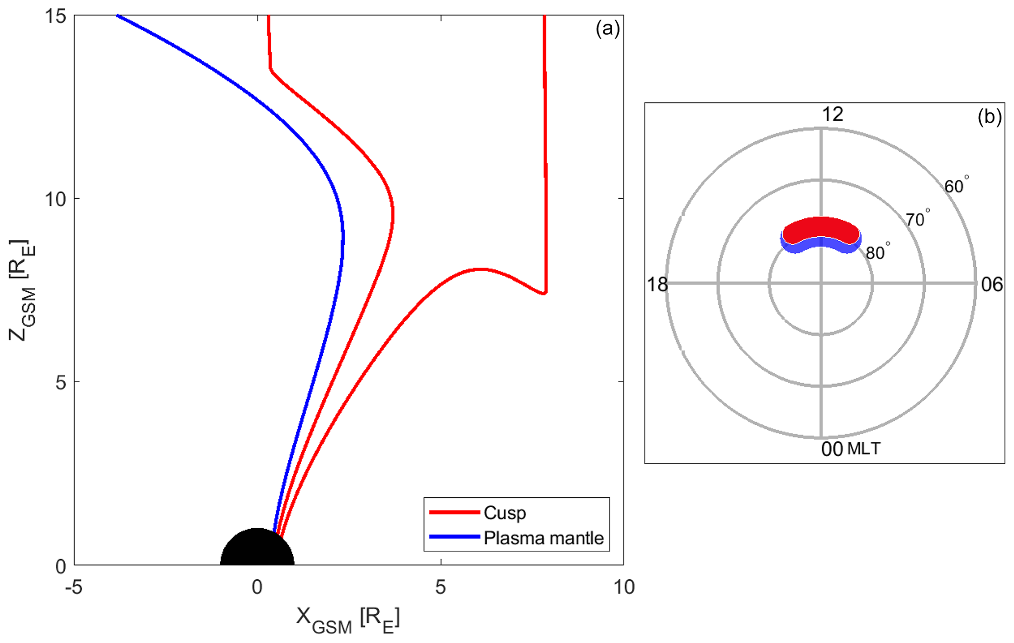
Figure 1Schematic representation of the cusp and plasma mantle regions determined from the T96 model. Panel (a) depicts boundary field lines in the XZGSM plane. Panel (b) depicts schematic (symmetric) areas of the cusp and plasma mantle in the polar cap. The cusp is represented with red and the plasma mantle with blue.
Using the TS96 model to extract 1 min cusp and plasma mantle measurements, the total number of EDI measurements is 1130 h (448 h are from the cusps), whereof 478 h (163 h from cusps) of data are from the Northern Hemisphere and 652 h (285 h from cusps) are from the Southern Hemisphere. The larger number of measurements from the Southern Hemisphere is a consequence of the Cluster orbit precession. We have more EDI observations from the plasma mantle than from the cusp, since the variable cusp magnetic field reduces the number of good quality EDI measurements (the “good quality” label is given in the Cluster Science Archive according to the series of criteria explained in the EDI user guide (Georgescu et al., 2010)).
Figure 2b shows the total distribution of all EDI measurements used. The data are shown in the cylindrical GSM coordinate system () and projected into the Northern Hemisphere. Here we ignored any north–south asymmetries and used only data with R>6 RE. The color bar indicates the number of 1 min data in each 1×1 RE bin. At least 3 min of data in each bin were required. The black line represents the average theoretical magnetopause position as in Shue et al. (1998), with input values of nT and PDYN=2 nPa.
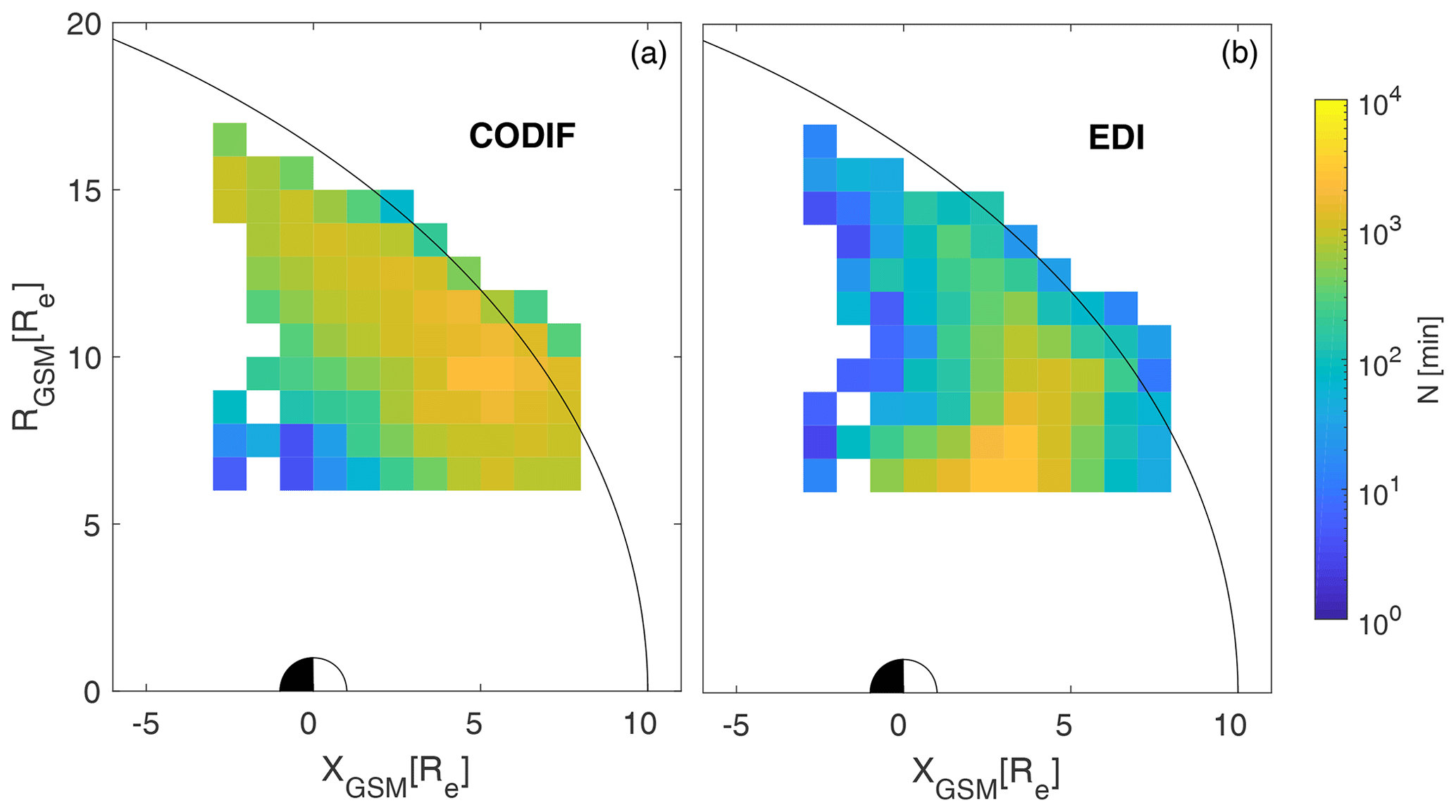
Figure 2Coverage of CODIF and EDI data projected into the Northern Hemisphere. The data are represented in a cylindrical coordinate system, where . The color bar indicates the number of 1 min measurements in each 1×1 RE bin. Panel (a) depicts CODIF coverage, while panel (b) depicts EDI coverage.
2.3 Cluster CODIF data
In order to measure parallel velocities and ion fluxes, the CODIF spectrometers (Rème et al., 1997) onboard the Cluster spacecraft were used. We use the same dataset as used in Slapak et al. (2017) in which plasma mantle data were obtained. A more detailed description of the dataset is given in Slapak et al. (2017), but for convenience we repeat some of the information.
The plasma mantel dataset was made using CODIF data from 2001 to 2005. Separating O+ CODIF data in the plasma mantle from the magnetosheath and the polar cap was done using a few criteria. First, the inner magnetosphere was removed by using only data where RE. In order to exclude polar cap data, the plasma β was used (derived from combined O+ and H+ CODIF data). Typical values of plasma β in the polar caps are below 0.01, and in the plasma mantle and magnetosheath it is above 0.1. Only data with β>0.1 are used. For separation between plasma sheet and plasma mantle data, Slapak et al. (2017) used H+ CODIF data. They noticed two clearly distinct peaks in H+ temperature for data with β>0.1. They decided on a H+ ion cut temperature of 1750 eV to separate the two populations. The two populations had different values of densities as well. One population had higher temperatures and lower densities, as expected in the plasma sheet, while the other population had lower temperatures and higher density, as expected in the plasma mantle. O+ shows similar features between the two populations. O+ densities in both populations are 1 order of magnitude lower than H+ densities, which is expected, and the plasma mantle population has a wider temperature range. Still, the two populations are easily distinguishable, and only data with eV are used. To separate magnetosheath data from plasma mantle data, Slapak et al. (2017) visually inspected O+ spectrograms. The magnetosheath is a region usually characterized by a more fluctuant magnetic field than inside of the magnetosphere. It is also characterized by strong H+ fluxes, which sometimes contaminate the O+ mass channel. In order to get parallel velocities (along the field lines), we used the scalar product of oxygen ion velocities and magnetic field direction: , where VO is an oxygen ion velocity measured with CODIF and b is the direction of the magnetic field. We then easily calculated the perpendicular velocity as . The perpendicular O+ velocities are comparable to the parallel velocities. We believe that the v⟂ values are too high and cannot be explained with the convection. As of now we do not know how to explain the perpendicular velocities and choose to ignore them in this study, and we use more accurate EDI measurements instead.
In total we have 1422 h of CODIF measurements. The distribution of CODIF measurements is shown in Fig. 2a. Here we can see the difference in data coverage between the two instruments (EDI and CODIF). The main reasons for this asymmetry are the technical restrictions of the instruments. The EDI has fewer measurements closer to the magnetopause because of higher variability of the magnetic field, while CODIF has more measurements closer to the magnetopause due to higher fluxes in this region. In addition to EDI and CODIF Cluster data, we also used solar wind dynamic pressure, Dst and IMF data from the OMNI dataset (King and Papitashvili, 2005). For IMF and solar wind dynamic pressure we used 1 min values and for Dst we implemented a simple linear interpolation in order to get the 1 min values.
The method used is a combination of the ones described in Haaland et al. (2012) and Li et al. (2012). If the outflowing ions can be traced to closed magnetic field lines before they reach the distant X-line at ca. −100 RE (e.g., Grigorenko et al., 2009; Daly, 1986), we infer that they are captured and returned to the magnetosphere. If they reach the X-line before being convected to the plasma sheet, the ions will be lost into the solar wind. For the highest energies, some of the ions will escape into the dayside magnetosheath directly before being convected into the plasma mantle. One issue here is the position of the distant X-line, which is not permanent but can vary with geomagnetic conditions. Since we do not know the exact location of the distant X-line in relation to the geomagnetic conditions, we have decided to use the fixed X-line and comment on its effect on the results in the discussion section. Another issue is the formation of the near-Earth X-line (around RE) during active geomagnetic conditions. At this point we are unable to determine what happens to the ions that are landing on two X-lines. The method we use to track the ions along their paths is based on the tracing of the ions along the field line using the TS96 model and moving the field lines with each time step in order to simulate the convection. We used the CODIF measurements of v∥ to move the ions along the field line in each time step and EDI measurements of v⟂ to move the field line accordingly. The method described in Haaland et al. (2012) infers that the capture will depend on the location of the ions in the YZGSM plane at RE. In their study the velocities and accelerations were calculated as averages. In Li et al. (2012) ions were traced for each measurement of the parallel and convection velocity. They calculated the acceleration for each tracing step. The direction and magnitude of the convection velocity are given by the following equation:
where the subscript 0 indicates the initial velocity and magnetic field, and i denotes the ith step. In the present paper we use a method similar to that of Haaland et al. (2007) to sample measurements and the method of Li et al. (2012) to trace particles.
Compared to the polar cap, Space Sci. Rev. have a broader energy range, 15 eV–5 keV (e.g., Bouhram et al., 2004; Lennartsson et al., 2004; Nilsson et al., 2012), so the mirror force and hence the acceleration and parallel velocity will vary correspondingly.
The location of the observations is very important since there is a region of enhanced perpendicular heating in the cusps in the range 8–12 RE (Arvelius et al., 2005; Nilsson et al., 2006; Waara et al., 2010), which results in higher perpendicular energies and thus higher parallel velocities due to the mirror force. If the outflowing ions are convected across the cusp to the plasma mantle before reaching this perpendicular heating region, they will not be significantly energized and will retain small energies and velocities. On the other hand, if they reach this heating region, they will be accelerated and can either be convected into the plasma mantle with large energies and velocities or escape into the dayside magnetosheath before being convected into closed magnetic field lines. In Nilsson et al. (2008), the centrifugal acceleration analysis in the cusp is discussed in some detail. There is significant acceleration between 8 and 10 RE. The acceleration in that region cannot be described by centrifugal acceleration alone and is most likely acceleration caused by wave–particle interaction. Figure 3 shows typical transport paths for oxygen ions of low, intermediate and high energies.
Our main assumption is that only centrifugal force accelerates oxygen ions on their path (mirror force acceleration is included in the centrifugal acceleration from Nilsson et al., 2008). A further assumption is that no other energization takes place along the particle path outside the cusps (e.g., no parallel E-fields or wave–particle acceleration). The gravitational force has no effects on the accelerations for the altitudes considered in our research, and without further energization the mirror force has little effect outside the cusps. We assume steady solar wind conditions during the tracing.
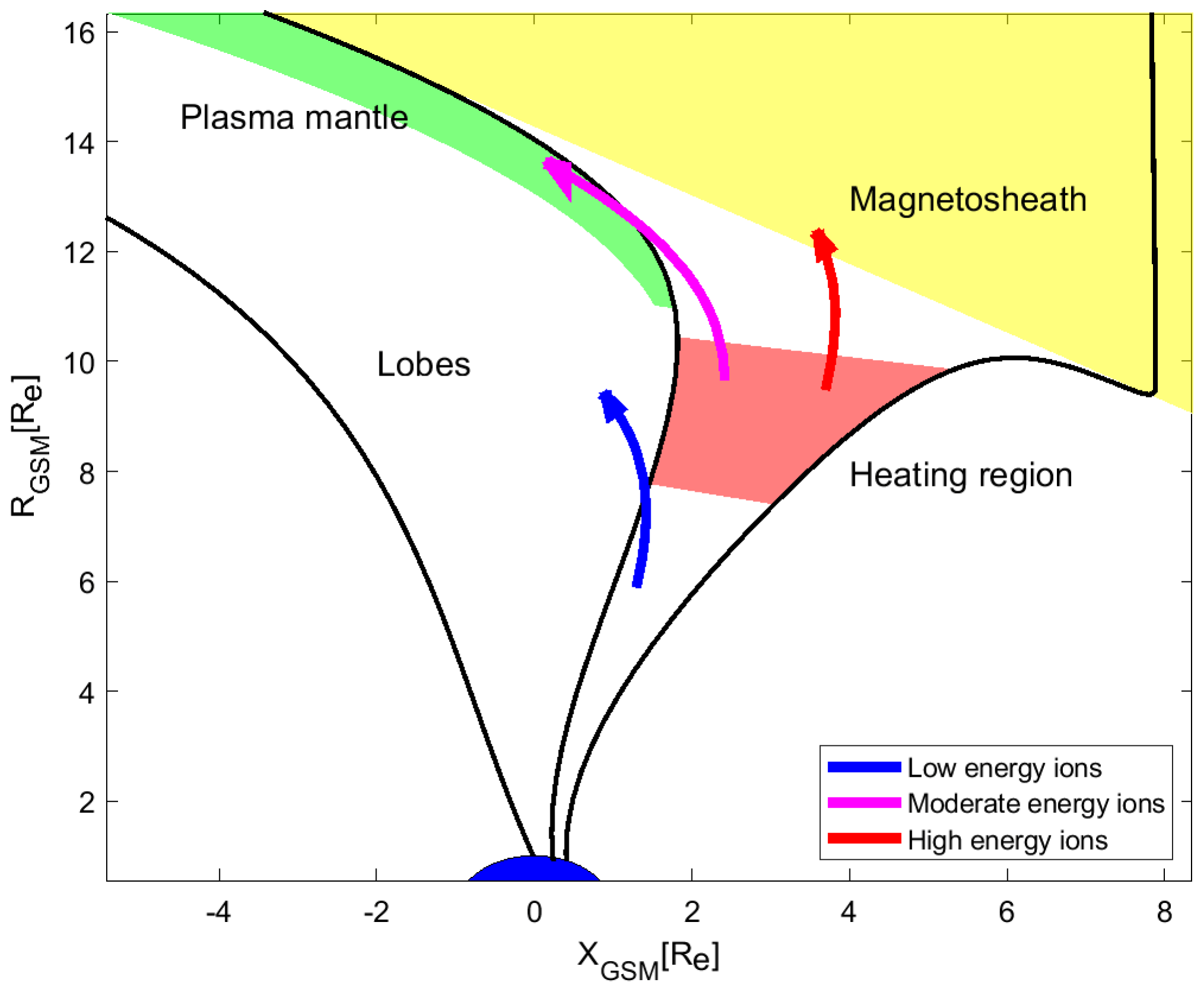
Figure 3Paths of oxygen ions based on their energies. The heating region in the high-altitude cusps as well as lobe and magnetosheath regions are included.
For particle acceleration along the field line, we use two values of the centrifugal accelerations: one value for the cusp and a different value for the lobe as in Nilsson et al. (2008, 2010). For cusp acceleration we used the following values:
For lobe acceleration, al, we used m , where the acceleration is scaled with radial distance given in Earth radii. The resulting velocity versus radial distance is shown in Fig. 4. The red line represents cusp velocities, and the blue line represents lobe velocities.
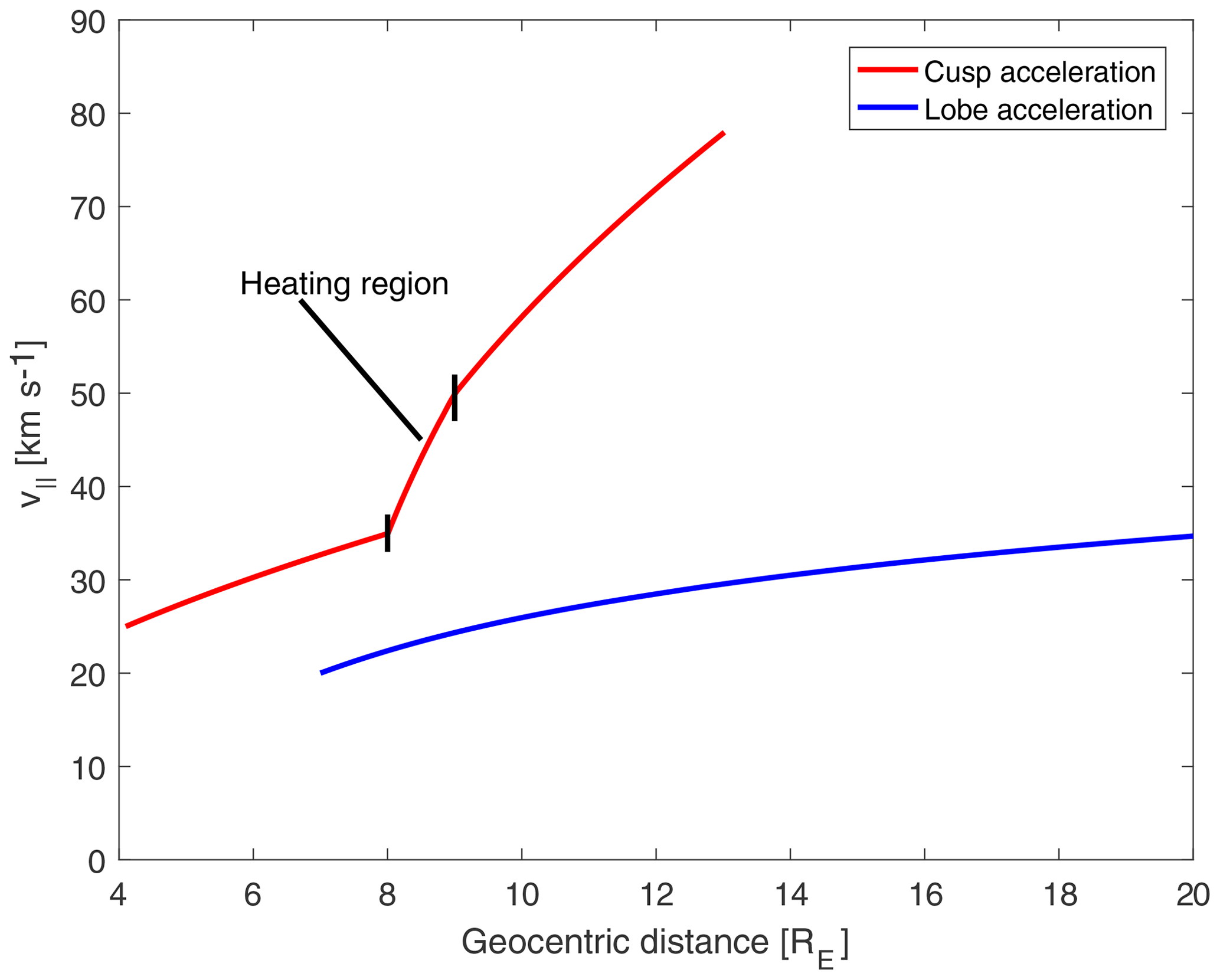
Figure 4Velocity dependence on radial distance in cusps and lobes, using acceleration values given in the text. The red line represents cusp velocities and the blue line represents lobe velocities.
From the EDI measurements in the cusp regions (based on the TS96 model), we have calculated the average convection velocity scaled to the ionosphere (height where B=50 000 nT, as in Slapak et al., 2017). The average cusp convection velocity in the ionosphere is 620 m s−1 in our dataset (at ≈400 km altitude). As an average cusp size in the ionosphere we used 4∘ in latitude (Burch, 1973). The average time to convect the most equatorward cusp field line across the cusp is 11 min. Newell and Meng (1987) calculated cusp widths as a function of the IMF Bz component. They investigated two case studies of changing IMF direction from the northward to southward directions. In the first case they had a stronger IMF for both the southward and northward directions, which resulted in a 3.5∘ latitudinal extent for the northward IMF and 2∘ for the southward IMF. In the second case they reported a 1.7∘ latitudinal extent of cusps for the northward IMF and 0.7∘ for the southward IMF. For the latter case, Newell and Meng (1987) concluded that for the northward IMF the cusp size decreased due to ongoing nightside reconnection, and for the southward IMF the cusp size decreased because strong convection rapidly closed the open cusp field lines. In this study we used values from the first case in Newell and Meng (1987): 3.5∘ for the northward IMF and 2∘ for the southward IMF. For average IMF conditions we have decided to use the 4∘ cusp latitudinal extent as given in Burch (1973). The cusp latitudinal extent, Δϕ, and scaling of cusp convection, , to the ionosphere, , are illustrated in Fig. 5.
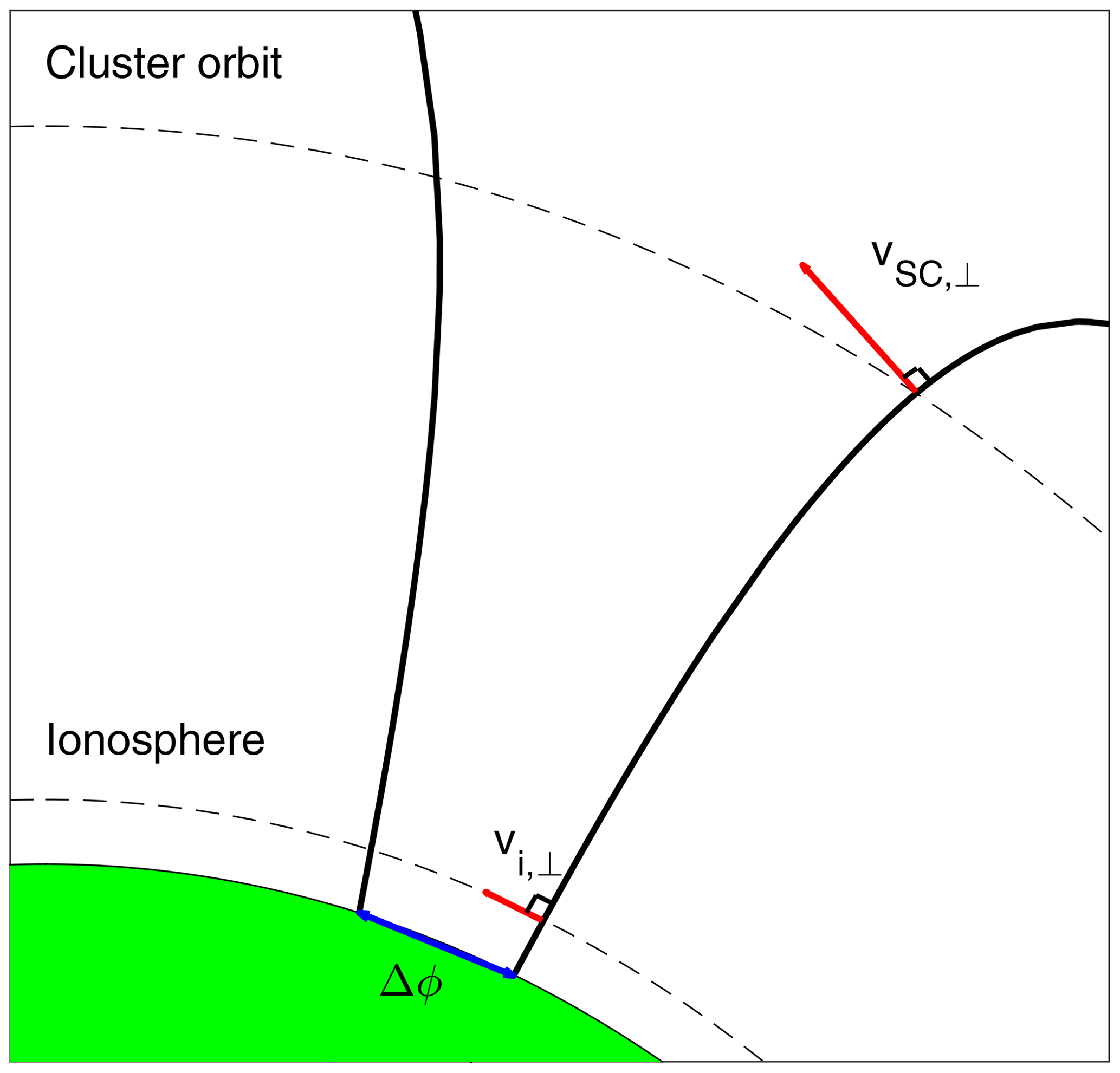
Figure 5Illustration of rescaling convection measurement to ionospheric height. The measured velocity at the spacecraft location, vSC⟂, is scaled to ionospheric height . Δϕ is cusp latitudinal extent at the surface of the Earth. Black lines represent the most sunward and most tailward cusp field lines, respectively.
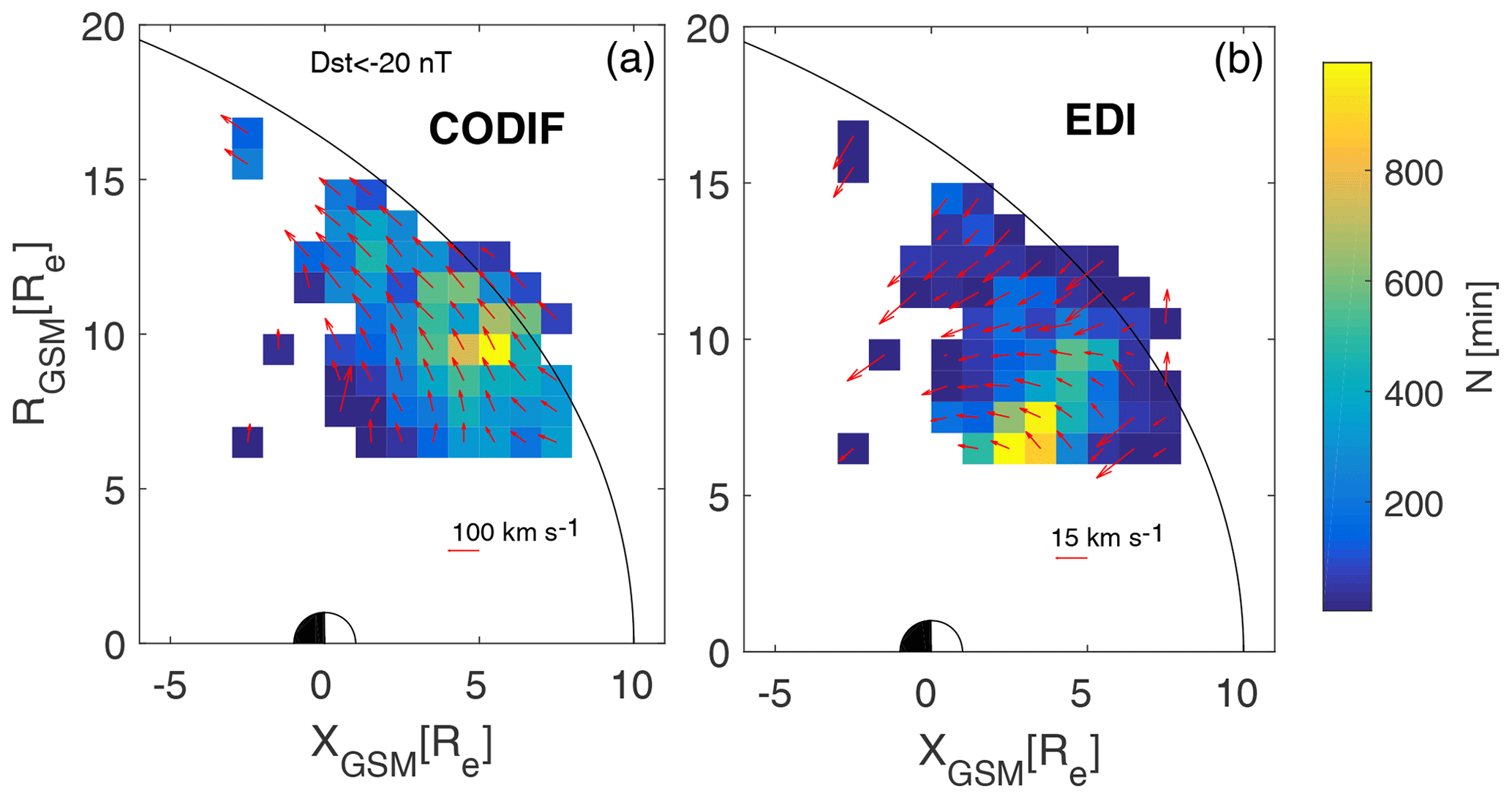
The starting point of our tracing is the center of each 1×1 RE spatial bin shown in Fig. 6. In order to avoid any dawn–dusk asymmetries, we use YGSM=0 and ZGSM=Rcyl as the starting point. The initial convection velocity is given by the measurements in each spatial bin. Convection velocities used are shown in Fig. 6. Convection velocities in each bin are calculated as the median of all measured drift magnitudes within a given bin. Average directions are calculated as the median value of the components of the normalized vectors. In Fig. 6, average convection velocities are shown with arrows. The length of the arrow indicates the magnitude of the vector; the scale is given in upper right corner. Colors of the bin represent the bias vector. The bias vector is calculated as the magnitude of the mean vector calculated from an ensemble of normalized vector components:
where v represents measured velocities and 〈…〉 denotes mean values. The bias vector is a good estimate of angular spread (see Haaland et al., 2007). Bias values close to zero value indicate a highly variable vector direction distribution, while values close to unity indicate vectors pointing in a coherent direction. Figure 6 shows that the direction of convection in the cusps is very variable. Bias vector values around 0.8 indicate an angular spread of around . We see that in the cusps the bias vector values are often lower than 0.8, indicating a very variable convection direction. This variability comes from the dynamic nature of the cusps. The cusp position and size are constantly changing due to solar wind conditions (IMF, PDyn) as well as temporal variations in tilt angle (daily and seasonal). Therefore, when averaging convection velocities without separation of the magnitude and direction, the average velocity will have a much smaller value than when averaging only the magnitude.
Since we use a magnetic field model, the initial convection velocity is given by the average (median) of the magnitudes within a bin, and the direction of the convection velocity is calculated using Eq. (1). The same equation is used to evaluate convection for further steps. For the parallel velocity we used median values from the CODIF dataset (Slapak et al., 2017) as magnitude, and a direction is given by the magnetic field model. For the subsequent time step we add acceleration. The first 11 min we use the cusp acceleration, given in Nilsson et al. (2008), and for the rest of the steps we use lobe acceleration values from Nilsson et al. (2010) – see Eq. (2). The distance travelled by a particle within one time step is then the product of the velocity times the time step. We have arbitrarily chosen a time step of 1 min. If the particle exits the magnetosphere within the first 11 min, we say that it has escaped into the dayside magnetosheath. If the particle ends up on the closed field line before reaching the X-line, we say it has returned to the magnetosphere. If the particle reaches the plasma sheet beyond the distant X-line, we say it escapes into the solar wind. A drawback with this simple separation of final regions is that they are based on a static model (T96), but this is as good as we can do with the present models.

Figure 6Distribution of average parallel and convection velocities in the cusps and plasma mantle regions. Lengths of vectors represent the convection velocity in each bin, calculated as the average magnitude of vectors. Colors indicate the bias value in each bin, a measure of directional variability. Panel (a) depicts parallel velocities obtained using CODIF data; panel (b) depicts convection velocities obtained using EDI data. Vectors are scaled as given in the lower right corner of each panel.
To estimate the percentages of oxygen outflow which end up in each of the three regions, solar wind, magnetosheath, and plasma sheet, we use the average measured oxygen flux in each bin. Depending on where each oxygen trace line ends, we add the average flux of that bin to the total flux of the respective region. Figure 7 shows oxygen flux distribution in the measurement bins.
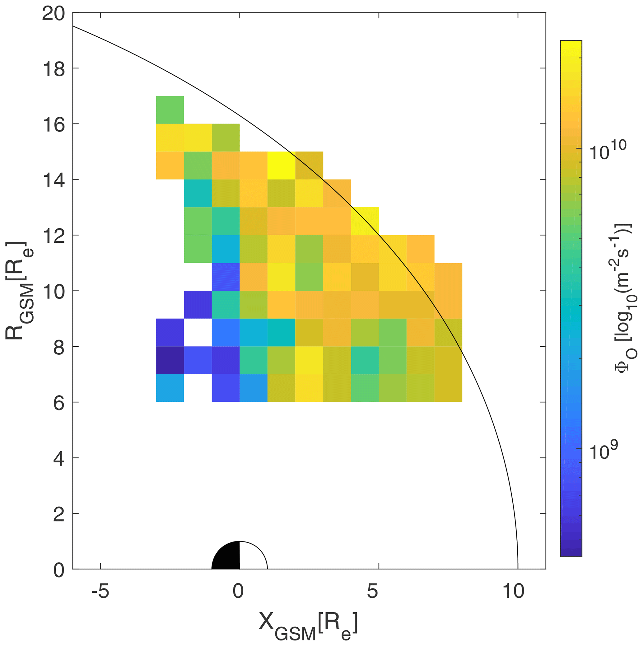
Figure 7Oxygen flux distribution in each measurement bin. Here we only use bins with both parallel and convection velocity data. The color bar indicates the amount of flux in each bin scaled to the ionospheric level (50 000 nT).
For the time input parameter to initialize the T96 model, we used the time of the equinox at noon for year 2011 (21 March 2011, 12:00:00). We have chosen the equinox because it represents (more or less) a yearly average state of magnetosphere in our dataset. We decided to use the spring equinox since in March the Cluster apogee is in the solar wind, and Cluster passes trough the dayside magnetosheath. Therefore, during spring the equinox we have more measurements than during the autumn equinox. We chose 2011 because it is in the middle between the minimum and maximum of the solar cycle.
The rest of the input parameters (Dst, IMF and solar wind pressure) are taken as the median of all values in the respective parameter. Results within a given Dst range are median values of a measurement within that Dst range. Input parameter values used for each condition are shown in Table 1. In Table 1 we also present the ionospheric cusp latitudinal extents from Newell and Meng (1987) (Δϕ in the table). Note that Newell and Meng (1987) correlated cusp width with the IMF Z component, while we use Dst to group the measurements. As seen from Table 1, the average IMF conditions for a given Dst range are in good agreement with Newell and Meng (1987). The other parameters in Table 1 are the average cusp convection scaled to ionospheric level (vi,c) and the maximum cusp convection time (tc).
Table 1Used input parameters in the geomagnetic model for different conditions. The first column shows the corresponding average of the full dataset.
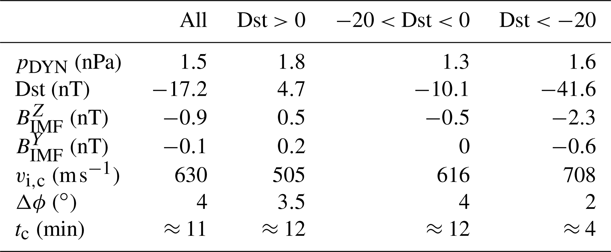
Figure 8 shows average particle traces for each 1×1 RE measurement bin. Colors indicate where the ions will end up. Blue color represents ions returned to the magnetosphere (captured), red color indicates the path of particles passing the X-line (lost), ending up in the solar wind, and black color indicates paths of ions transported to the dayside magnetosheath (lost). Panel a shows a case with average starting parallel velocity, panel b shows a case with parallel velocity 1 standard deviation below the average, and panel c shows a case for parallel velocities 1 standard deviation above the average. We see that black lines do not show any reasonable behavior outside the magnetosphere since the T96 magnetic model fails outside the magnetosphere. Consequently, the traces are unreliable, but the ions definitely end up in the magnetosheath. Most of the oxygen ions escape into the solar wind beyond the distant X-line. A fraction of the oxygen ions is convected to the plasma sheet, and a small part will escape into the dayside magnetosheath. From our results, it takes 120 min on average for oxygen ions to reach the distant X-line (based on average parallel 〈vpar〉 velocities). That means that if oxygen ions are not convected into the plasma sheet within 120 min they will most likely escape beyond the distant X-line.
In Fig. 9 we show the results of the tracing on the sampling bins (starting positions of the tracing); i.e., the colors indicate where the tracing will end starting from each bin. Colors used are the same as in Fig. 8. The average cusp ion outflow is 3.9×1024 s−1 and the estimated percentages of oxygen flux which end up in each region are given in Table 2.
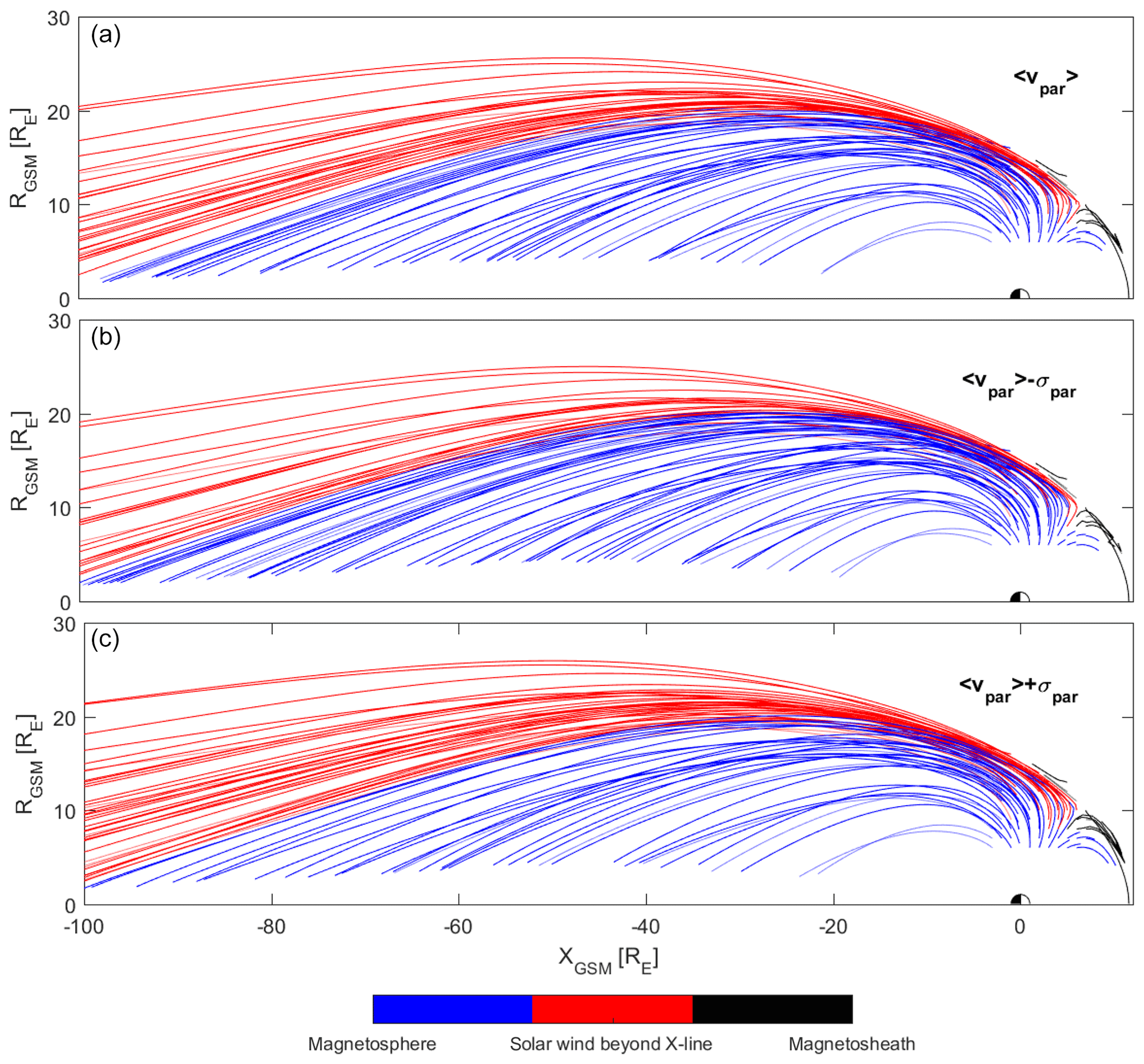
Figure 8Tracing results using initial parallel velocities. Individual lines show the paths of particles from each measurement bin. Colors indicate the fate of oxygen ions: blue indicates that they will return to the magnetosphere (mostly plasma sheet), red indicates ions ending up in the solar wind, and black indicates ions escaping into the dayside magnetosheath. Different panels represent cases for different starting velocities: (a) shows results using average velocities, (b) shows results using lower standard deviation velocities and (c) shows results using upper standard deviation velocities.
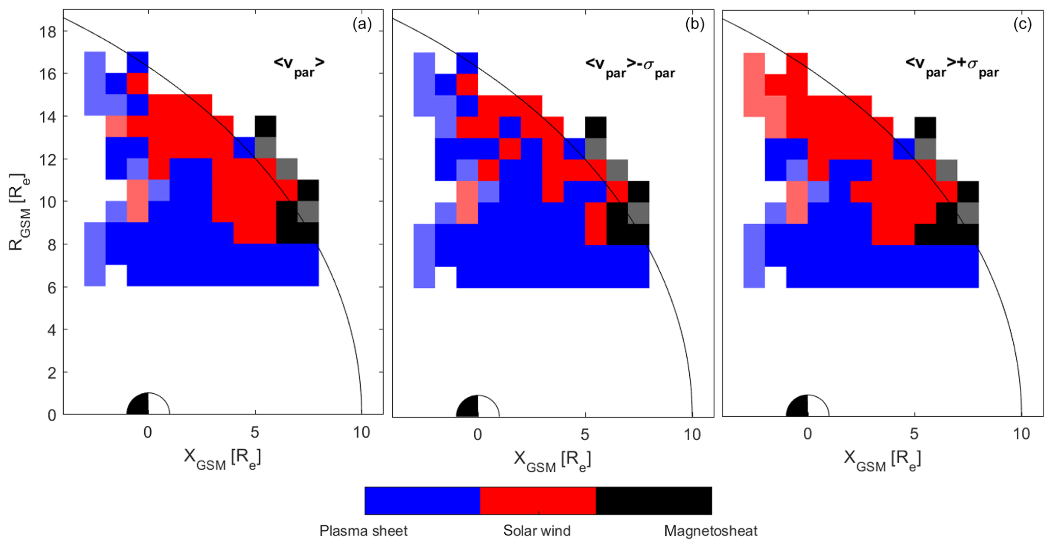
Figure 9The figure depicts the results of tracing for each starting bin. The different panels show various starting parallel velocities. Cases for the starting parallel velocities from (a) to (c) are average parallel velocity, lower standard deviation parallel velocity and upper standard deviation parallel velocity. Transparent colors represent the bins with less than 30 min of EDI measurement.
Table 2Estimated fate of oxygen ions expressed as percentages of outflow flux. Φ represents the flux, and subscripts ms, sw and ps represent magnetosheath, solar wind and plasma sheet, respectively. σpar represents the standard deviation of the parallel initial velocities.
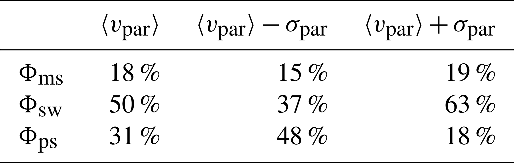
From our estimation, on average 31 % of the total oxygen flux from the high-altitude cusp gets convected to the plasma sheet. The further fate of these ions and transport inside the plasma sheet is beyond the scope of this paper, but it is reasonable to assume that a fraction of the recirculated ions are eventually lost through plasmoid ejections, through the magnetopause and through other loss processes.
We also present the resulting oxygen outflow for different storm conditions, using the Dst index as a proxy for storm conditions. For quiet conditions we used positive Dst values, for moderate storm conditions we used Dst values between 0 and −20 nT, and for active storm conditions we used Dst values below −20 nT. For quiet and active storm conditions for nightside measurement bins ( RE) the coverage is rather poor, but this is not a major problem, since the oxygen fluxes are rather low under these conditions, thus not affecting the overall results significantly. The threshold for active storm conditions might seem a bit high, but for a lower threshold we have a much smaller dataset and a lot more data gaps (see Appendix Figs. A1–A3). The results of the tracing for different storm conditions are given in Fig. 10. As seen from this figure, the results are highly dependent on storm conditions. The gaps for active and quiet conditions would probably favor capture, since for moderate storm conditions this region bins all show capture, but it would only change results by a couple of percent, due to the lower fluxes in those bins (see Fig. 7). The most interesting case is the tracing during active storm conditions, because most of the outflowing oxygen flux gets convected into the plasma sheet. During strong storms, both parallel velocity and convection velocities increase, but the increase in convection is stronger, causing a larger flux of oxygen ions into the plasma sheet. The outflowing O+ ions are deposited closer to Earth, for storm geomagnetic conditions. In Fig. 11 we show the results of the tracing in starting bins in the same way as in Fig. 9, but for various geomagnetic conditions. The estimated percentages of the fate of oxygen flux for various Dst conditions are given in Table 3.
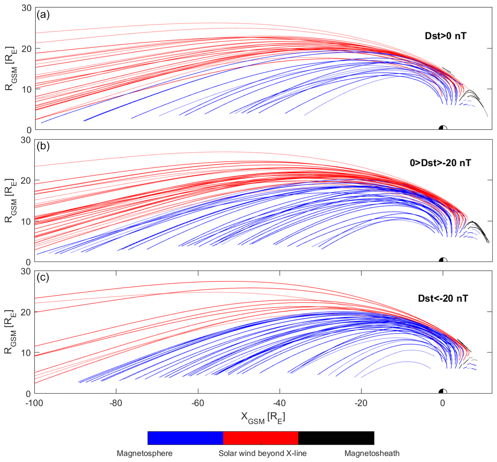
Figure 10The tracing results using parallel initial velocities for different storm conditions. Panel (a) shows quiet conditions, panel (b) shows moderate storm conditions, and panel (c) shows active storm conditions. The colors are the same as in Fig. 8.
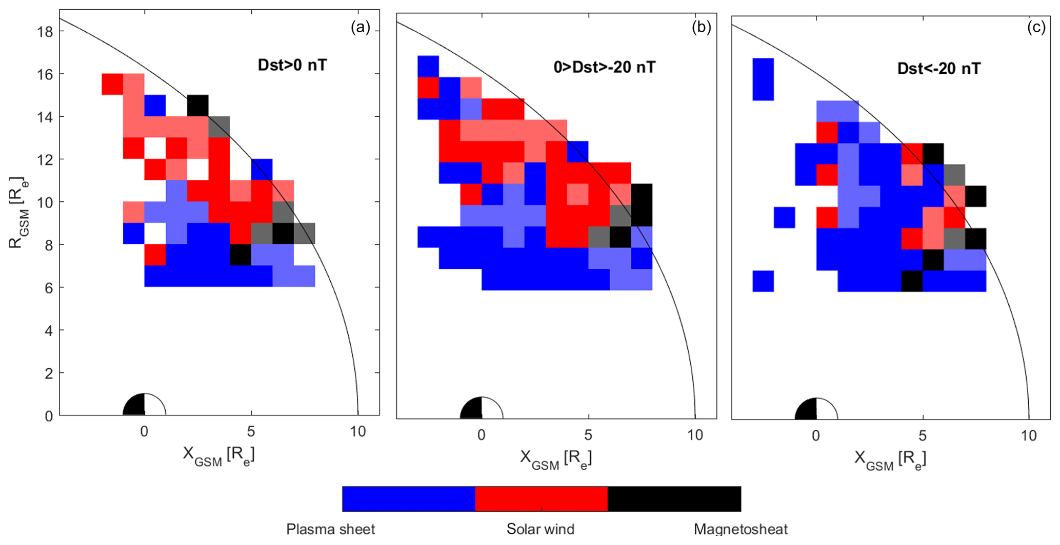
Figure 11Results of tracing for each starting bin. Different panels depict various starting geomagnetic conditions. Cases for the starting parallel velocities from (a) to (c) are quiet conditions, moderate conditions and active geomagnetic conditions. The colors are the same as in Fig. 8.
Table 3Estimated fate of oxygen ions expressed as percentages of outflow flux. Φ represents the flux, and subscripts ms, sw and ps represent magnetosheath, solar wind and plasma sheet, assuming that the plasma sheet is limited by the distant X-line at RE.

In terms of oxygen outflow escape from the high-altitude cusps and plasma mantle regions, we find that most of the oxygen escapes the magnetosphere, as shown by Slapak et al. (2017). As pointed out by Seki et al. (2002) and Ebihara et al. (2006), oxygen ions with low energies (<1 keV) will end up in the near-tail plasma sheet or in the ring current. Our results show that oxygen ions reaching the high-altitude cusps will mostly escape the magnetosphere. On average, 50 % of the oxygen outflow flux will end up in the solar wind beyond the distant X-line; 19 % will escape directly into the dayside magnetosheath. This sums up to a total escape rate of 69 % of high-altitude cusp oxygen flux. The rest, 31 % of the high-altitude cusp flux, is being convected to the plasma sheet, mostly in the distant tail (>50 RE), as shown by Fig. 8.
Another important issue is the escape-versus-capture ratio for different storm conditions. During quiet magnetospheric conditions, oxygen outflow and energization are relatively low, resulting in lower fluxes of oxygen in the high-altitude cusp. However, in such cases, the magnetospheric convection is also low, and consequently almost all of the outflowing oxygen escapes. It is worth mentioning that in such cases IMF is mostly northward and can lead to lobe reconnection, resulting in sunward flow. This process can decelerate oxygen ions and lead to their capture. Positive Dst periods are also often characterized by sudden high PDYN changes (e.g., Boudouridis et al., 2007; Gillies et al., 2012). We did not did not differentiate sudden commencement from quiet conditions, since we used the average values of a large dataset. We assume that such changes are increasing our average convection velocities and the oxygen outflow (which are low), and without them the results would not change much all together. During moderate storm conditions, results are similar to average conditions. For active storm conditions, the oxygen ion flux is high, and both the parallel velocity of the oxygen ions and the convection are higher. This leads to an increase in both dayside magnetosheath escape and enhanced convection into the plasma sheet. Oxygen ions are more likely to escape into the dayside magnetosheath due to their high parallel velocities. Oxygen ions that get convected from the cusps into the plasma mantle will eventually be convected into the plasma sheet. There are also other processes which can further energize ions on their path during strong magnetospheric storms and thus cause them to escape beyond the X-line. For example, Lindstedt et al. (2010) reported additional energization of a few keV at the cusp–lobe boundary during strong geomagnetic storms, caused by increased reconnection leading to a strong localized Hall electric field and non-adiabatic motion of the ions.
Lennartsson et al. (2004) reported observations of oxygen ions with energies of 3–4 keV in the magnetospheric lobes around 10 RE during geomagnetic storms. In our tracing, ions with such high energies in the tail around 10 RE are traveling close to the magnetopause, and the results of Lennartsson et al. (2004) cannot be verified by our study. During geomagnetic storms, 73 % of the oxygen flux ends up in the plasma sheet but far down in the tail (beyond 50 RE). The high-energy oxygen ions in the lobes reported by Lennartsson et al. (2004) are more likely the result of magnetospheric energization of existing low-energy oxygen ions in the lobes rather than convection of high-energy oxygen ions. The overall dependence of oxygen capture during storm conditions agrees with results from Haaland et al. (2012), in the sense that we observe increased capture during active storm conditions and more escape during quiet conditions. The main difference is that Haaland et al. (2012) analyzed the capture rate of low-energy hydrogen ions in the lobes emanating from the polar cap regions, while in this paper we have analyzed the fate of energy oxygen ions emanating from the cusp regions.
In this paper we have used Cluster EDI data in the lobes in combination with the CODIF cusp dataset from Slapak et al. (2017) to obtain parallel and convection velocities for oxygen ions. Furthermore, we used results from Nilsson et al. (2006, 2008) for accelerations in cusps and lobes, as well as results from Newell and Meng (1987) for cusp width, to estimate the fate of oxygen ions originating from the high-altitude cusp regions. The findings are summarized as follows.
-
Assuming that the magnetosphere terminates at a distant X-line fixed at RE, 69 % of total oxygen outflow from the high-altitude cusps escapes the magnetosphere on average; 50 % escapes tailward beyond the distant X-line and 19 % escapes to the dayside magnetosheath.
-
The oxygen capture-versus-escape ratio is highly dependent on geomagnetic conditions. Oxygen ions originating in the cusp are more likely to be captured during active conditions since the majority of oxygen outflow is convected to the plasma sheet, although rather far downtail.
-
The average time for oxygen ions to reach the distant X-line (−100 RE) is 120 min.
Figures A1, A2, and A3 show the datasets we used for different storm conditions. Panel a in each figure shows the CODIF dataset and panel b shows the EDI dataset. Red vectors represent the average vector in each sampling bin, scaled with the vector shown in the lower right corner in each panel. The color of the bin represents the number of 1 min data in that bin. Figure A1 shows the data distribution for quiet geomagnetic conditions, Fig. A2 shows the data distribution for moderate geomagnetic conditions, and Fig. A3 shows that for active geomagnetic conditions.
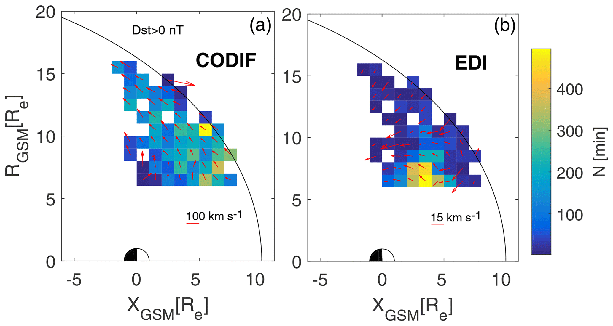
Figure A1Distribution of average parallel and convection velocities in the cusps and plasma mantle regions for quiet geomagnetic conditions. Lengths of vectors represent convection velocity in each bin, calculated as the average magnitude of vectors. Colors indicate the number of 1 min measurements in each bin. Panel (a) depicts parallel velocities obtained using CODIF data; panel (b) depicts convection velocities obtained using EDI data. Vectors are scaled as given in the lower right corner of each panel.
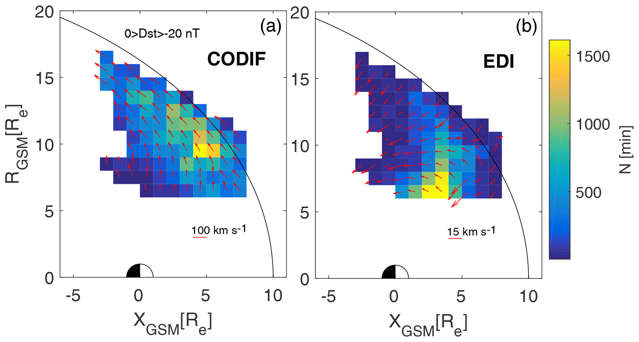
Figure A2Distribution of average parallel and convection velocities in the cusps and plasma mantle regions for moderate geomagnetic conditions. Labels are the same as in Fig. A1.
The Cluster EDI and CODIF data are provided by ESA's Cluster Science Archive and can be accessed at https://csa.esac.esa.int/csa-web/#search (ESA, 2019). We acknowledge use of NASA/GSFC's Space Physics Data Facility OMNIWeb service and OMNI data, which can be accessed at https://cdaweb.gsfc.nasa.gov (NASA, 2019).
PK and SH conceived the presented idea. PK analyzed EDI data and performed the oxygen ion tracing. RS and AS analyzed and prepared the CODIF data. SH supervised the project. PK improved the method in discussions with SH and LM. All the authors contributed to discussions and PK wrote the paper with input from all the authors.
The authors declare that they have no conflict of interest.
Patrik Krcelic acknowledges support from the University of Zagreb, Croatia, Erasmus+ program. Patrik Krcelic thanks the Max Planck Institute for Solar System Research, Göttingen, Germany, for hosting him for the duration of this work. Stein Haaland was supported by the Norwegian Research Council (NFR) under grant 223252 and the German Aerospace Center (DLR) under contract 50 OC 0302. Lukas Maes acknowledges the support by the Deutsches Zentrum für Luft- und Raumfahrt, grant DLR 50QM170. Rikard Slapak acknowledges the financial support from the EISCAT Scientific Association, Kiruna, Sweden. Audrey Schillings acknowledges the financial support from the Swedish Institute of Space Physics, Graduate School of Space Technology in Luleå, Sweden. Patrik Krcelic would like to thank the whole MPS group for all their support and for making this paper possible.
Cluster EDI has been supported by the
European Space Agency (ESA) through the
Cluster Science Archive activities and
by the Deutsches Zentrum für Luft- und
Raumfahrt (DLR) (grant no. 50 OC 1602).
The article processing charges for this open-access
publication were covered by the Max Planck Society.
This paper was edited by Minna Palmroth and reviewed by Maxime Grandin and one anonymous referee.
Andre, M., Crew, G., Peterson, W., Persoon, A., and Pollock, C.: Heating of ion conics in the cusp/cleft, Physics of Space Plasmas, (1989), 203–213, 1990. a
Arvelius, S., Yamauchi, M., Nilsson, H., Lundin, R., Hobara, Y., Rème, H., Bavassano-Cattaneo, M. B., Paschmann, G., Korth, A., Kistler, L. M., and Parks, G. K.: Statistics of high-altitude and high-latitude O+ ion outflows observed by Cluster/CIS, Ann. Geophys., 23, 1909–1916, https://doi.org/10.5194/angeo-23-1909-2005, 2005. a
Axford, W. I.: The polar wind and the terrestrial helium budget, J. Geophys. Res. (1896–1977), 73, 6855–6859, https://doi.org/10.1029/JA073i021p06855, 1968. a
Boudouridis, A., Lyons, L. R., Zesta, E., and Ruohoniemi, J. M.: Dayside reconnection enhancement resulting from a solar wind dynamic pressure increase, J. Geophys. Res.-Sp. Phys., 112, A06201, https://doi.org/10.1029/2006JA012141, 2007. a
Bouhram, M., Malingre, M., Jasperse, J. R., Dubouloz, N., and Sauvaud, J.-A.: Modeling transverse heating and outflow of ionospheric ions from the dayside cusp/cleft. 2 Applications, Ann. Geophys., 21, 1773–1791, https://doi.org/10.5194/angeo-21-1773-2003, 2003. a
Bouhram, M., Klecker, B., Miyake, W., Rème, H., Sauvaud, J.-A., Malingre, M., Kistler, L., and Blăgău, A.: On the altitude dependence of transversely heated O+ distributions in the cusp/cleft, Ann. Geophys., 22, 1787–1798, https://doi.org/10.5194/angeo-22-1787-2004, 2004. a
Burch, J. L.: Rate of erosion of dayside magnetic flux based on a quantitative study of the dependence of polar cusp latitude on the interplanetary magnetic field, Radio Sci., 8, 955–961, https://doi.org/10.1029/RS008i011p00955, 1973. a, b, c
Chappell, C. R., Moore, T. E., and Waite Jr., J. H.: The ionosphere as a fully adequate source of plasma for the Earth's magnetosphere, J. Geophys. Res.-Sp. Phys., 92, 5896–5910, https://doi.org/10.1029/JA092iA06p05896, 1987. a
Chappell, C. R., Giles, B. L., Moore, T. E., Delcourt, D. C., Craven, P. D., and Chandler, M. O.: The adequacy of the ionospheric source in supplying magnetospheric plasma, J. Atmos. So.-Terr. Phys., 62, 421–436, https://doi.org/10.1016/S1364-6826(00)00021-3, 2000. a
Cladis, J. B.: Parallel acceleration and transport of ions from polar ionosphere to plasma sheet, Geophys. Res. Lett., 13, 893–896, https://doi.org/10.1029/GL013i009p00893, 1986. a
Daly, P. W.: Structure of the distant terrestrial magnetotail, Adv. Space Res., 6, 245–257, https://doi.org/10.1016/0273-1177(86)90041-4, 1986. a
Ebihara, Y., Yamada, M., Watanabe, S., and Ejiri, M.: Fate of outflowing suprathermal oxygen ions that originate in the polar ionosphere, J. Geophys. Res.-Sp. Phys., 111, A04219, https://doi.org/10.1029/2005JA011403, 2006. a, b
Engwall, E., Eriksson, A. I., Cully, C. M., André, M., Puhl-Quinn, P. A., Vaith, H., and Torbert, R.: Survey of cold ionospheric outflows in the magnetotail, Ann. Geophys., 27, 3185–3201, https://doi.org/10.5194/angeo-27-3185-2009, 2009. a
ESA: Cluster EDI and CODIF data, available at: https://csa.esac.esa.int/csa-web/#search, last access: 2019. a
Escoubet, C. P., Fehringer, M., and Goldstein, M.: Introduction The Cluster mission, Ann. Geophys., 19, 1197–1200, https://doi.org/10.5194/angeo-19-1197-2001, 2001. a
Georgescu, E., Puhl-Quinn, P., Vaith, H., Chutter, M., Quinn, J., Paschmann, G., and Torbert, R.: EDI Data Products in the Cluster Active Archive, The Cluster Active Archive, Studying the Earth's Space Plasma Environment, Astrophysics and Space Science Proceedings, Springer, Dordrecht, 83–95, https://doi.org/10.1007/978-90-481-3499-1_5, 2010. a
Gillies, D. M., St.-Maurice, J.-P., McWilliams, K. A., and Milan, S.: Global-scale observations of ionospheric convection variation in response to sudden increases in the solar wind dynamic pressure, J. Geophys. Res.-Sp. Phys., 117, A04209, https://doi.org/10.1029/2011JA017255, 2012. a
Glocer, A., Tóth, G., Gombosi, T., and Welling, D.: Modeling ionospheric outflows and their impact on the magnetosphere, initial results, J. Geophys. Res.-Sp. Phys., 114, A05216, https://doi.org/10.1029/2009JA014053, 2009. a
Grigorenko, E. E., Hoshino, M., Hirai, M., Mukai, T., and Zelenyi, L. M.: “Geography” of ion acceleration in the magnetotail: X-line versus current sheet effects, J. Geophys. Res.-Sp. Phys., 114, A03203, https://doi.org/10.1029/2008JA013811, 2009. a
Gustafsson, G., Boström, R., Holback, B., Holmgren, G., Lundgren, A., Stasiewicz, K., Åhlén, L., Mozer, F. S., Pankow, D., Harvey, P., Berg, P., Ulrich, R., Pedersen, A., Schmidt, R., Butler, A., Fransen, A. W. C., Klinge, D., Thomsen, M., Fälthammar, C.-G., Lindqvist, P.-A., Christenson, S., Holtet, J., Lybekk, B., Sten, T. A., Tanskanen, P., Lappalainen, K., and Wygant, J.: The electric field and wave experiment for the cluster mission, Space Sci. Rev., 79, 137–156, https://doi.org/10.1023/A:1004975108657, 1997. a
Haaland, S., Eriksson, A., Engwall, E., Lybekk, B., Nilsson, H., Pedersen, A., Svenes, K., André, M., Förster, M., Li, K., Johnsen, C., and Østgaard, N.: Estimating the capture and loss of cold plasma from ionospheric outflow, J. Geophys. Res.-Sp. Phys., 117, A07311, https://doi.org/10.1029/2012JA017679, 2012. a, b, c, d, e
Haaland, S. E., Paschmann, G., Förster, M., Quinn, J. M., Torbert, R. B., McIlwain, C. E., Vaith, H., Puhl-Quinn, P. A., and Kletzing, C. A.: High-latitude plasma convection from Cluster EDI measurements: method and IMF-dependence, Ann. Geophys., 25, 239–253, https://doi.org/10.5194/angeo-25-239-2007, 2007. a, b
King, J. H. and Papitashvili, N. E.: Solar wind spatial scales in and comparisons of hourly Wind and ACE plasma and magnetic field data, J. Geophys. Res.-Sp. Phys., 110, https://doi.org/10.1029/2004JA010649, 2005. a
Kistler, L. M., Mouikis, C. G., Klecker, B., and Dandouras, I.: Cusp as a source for oxygen in the plasma sheet during geomagnetic storms, J. Geophys. Res.-Sp. Phys., 115, A03209, https://doi.org/10.1029/2009JA014838, 2010. a
Kitamura, N., Ogawa, Y., Nishimura, Y., Terada, N., Ono, T., Shinbori, A., Kumamoto, A., Truhlik, V., and Smilauer, J.: Solar zenith angle dependence of plasma density and temperature in the polar cap ionosphere and low-altitude magnetosphere during geomagnetically quiet periods at solar maximum, J. Geophys. Res.-Sp. Phys., 116, A08227, https://doi.org/10.1029/2011JA016631, 2011. a
Laakso, H. and Grard, R.: The electron density distribution in the polar cap: Its variability with seasons, and its response to magnetic activity, in: Space Weather Study Using Multipoint Techniques, edited by: Lyu, L.-H., vol. 12 of COSPAR Colloquia Series, 193–202, Pergamon, https://doi.org/10.1016/S0964-2749(02)80218-9, 2002. a
Lennartsson, O. W., Collin, H. L., and Peterson, W. K.: Solar wind control of Earth's H+ and O+ outflow rates in the 15-eV to 33-keV energy range, J. Geophys. Res.-Sp. Phys., 109, A12212, https://doi.org/10.1029/2004JA010690, 2004. a, b, c, d
Li, K., Haaland, S., Eriksson, A., André, M., Engwall, E., Wei, Y., Kronberg, E. A., Fränz, M., Daly, P. W., Zhao, H., and Ren, Q. Y.: On the ionospheric source region of cold ion outflow, Geophys. Res. Lett., 39, L18102, https://doi.org/10.1029/2012GL053297, 2012. a, b, c
Liao, J., Kistler, L., Mouikis, C., Klecker, B., Dandouras, I., and Zhang, J.-C.: Statistical study of O+ transport from the cusp to the lobes with Cluster CODIF data, J. Geophys. Res.-Sp. Phys., 115, A00J15, https://doi.org/10.1029/2010JA015613, 2010. a
Lindstedt, T., Khotyaintsev, Y. V., Vaivads, A., André, M., Nilsson, H., and Waara, M.: Oxygen energization by localized perpendicular electric fields at the cusp boundary, Geophys. Res. Lett., 37, L09103, https://doi.org/10.1029/2010GL043117, 2010. a
Lockwood, M., Waite Jr., J. H., Moore, T. E., Johnson, J. F. E., and Chappell, C. R.: A new source of suprathermal O+ ions near the dayside polar cap boundary, J. Geophys. Res.-Sp. Phys., 90, 4099–4116, https://doi.org/10.1029/JA090iA05p04099, 1985. a, b
Moore, T. E. and Horwitz, J. L.: Stellar ablation of planetary atmospheres, Rev. Geophys., 45, RG3002, https://doi.org/10.1029/2005RG000194, 2007. a
NASA: OMNI data, available at: https://cdaweb.gsfc.nasa.gov, last access: 2019. a
Newell, P. T. and Meng, C.-I.: Cusp width and Bz : Observations and a conceptual model, J. Geophys. Res.-Sp. Phys., 92, 13673–13678, https://doi.org/10.1029/JA092iA12p13673, 1987. a, b, c, d, e, f, g, h
Nilsson, H.: Heavy Ion Energization, Transport, and Loss in the Earth's Magnetosphere, 315–327, Springer Netherlands, Dordrecht, https://doi.org/10.1007/978-94-007-0501-2_17, 2011. a, b
Nilsson, H., Yamauchi, M., Eliasson, L., Norberg, O., and Clemmons, J.: Ionospheric signature of the cusp as seen by incoherent scatter radar, J. Geophys. Res.-Sp. Phys., 101, 10947–10963, https://doi.org/10.1029/95JA03341, 1996. a
Nilsson, H., Waara, M., Arvelius, S., Marghitu, O., Bouhram, M., Hobara, Y., Yamauchi, M., Lundin, R., Rème, H., Sauvaud, J.-A., Dandouras, I., Balogh, A., Kistler, L. M., Klecker, B., Carlson, C. W., Bavassano-Cattaneo, M. B., and Korth, A.: Characteristics of high altitude oxygen ion energization and outflow as observed by Cluster: a statistical study, Ann. Geophys., 24, 1099–1112, https://doi.org/10.5194/angeo-24-1099-2006, 2006. a, b
Nilsson, H., Waara, M., Marghitu, O., Yamauchi, M., Lundin, R., Rème, H., Sauvaud, J.-A., Dandouras, I., Lucek, E., Kistler, L. M., Klecker, B., Carlson, C. W., Bavassano-Cattaneo, M. B., and Korth, A.: An assessment of the role of the centrifugal acceleration mechanism in high altitude polar cap oxygen ion outflow, Ann. Geophys., 26, 145–157, https://doi.org/10.5194/angeo-26-145-2008, 2008. a, b, c, d, e, f
Nilsson, H., Engwall, E., Eriksson, A., Puhl-Quinn, P. A., and Arvelius, S.: Centrifugal acceleration in the magnetotail lobes, Ann. Geophys., 28, 569–576, https://doi.org/10.5194/angeo-28-569-2010, 2010. a, b, c
Nilsson, H., Barghouthi, I. A., Slapak, R., Eriksson, A. I., and André, M.: Hot and cold ion outflow: Spatial distribution of ion heating, J. Geophys. Res.-Sp. Phys., 117, A11201, https://doi.org/10.1029/2012JA017974, 2012. a
Norqvist, P., André, M., Eliasson, L., Eriksson, A. I., Blomberg, L., Lühr, H., and Clemmons, J. H.: Ion cyclotron heating in the dayside magnetosphere, J. Geophys. Res.-Sp. Phys., 101, 13179–13193, https://doi.org/10.1029/95JA03596, 1996. a
Ogawa, Y., Fujii, R., Buchert, S. C., Nozawa, S., and Ohtani, S.: Simultaneous EISCAT Svalbard radar and DMSP observations of ion upflow in the dayside polar ionosphere, J. Geophys. Res., 108, 1101, https://doi.org/10.1029/2002JA009590, 2003. a
Paschmann, G., Melzner, F., Frenzel, R., Vaith, H., Parigger, P., Pagel, U., Bauer, O. H., Haerendel, G., Baumjohann, W., Scopke, N., Torbert, R. B., Briggs, B., Chan, J., Lynch, K., Morey, K., Quinn, J. M., Simpson, D., Young, C., Mcilwain, C. E., Fillius, W., Kerr, S. S., Mahieu, R., and Whipple, E. C.: The electron drift instrument for cluster, Space Sci. Rev., 79, 233–269, https://doi.org/10.1023/A:1004917512774, 1997. a
Paschmann, G., Quinn, J. M., Torbert, R. B., Vaith, H., McIlwain, C. E., Haerendel, G., Bauer, O. H., Bauer, T., Baumjohann, W., Fillius, W., Förster, M., Frey, S., Georgescu, E., Kerr, S. S., Kletzing, C. A., Matsui, H., Puhl-Quinn, P., and Whipple, E. C.: The Electron Drift Instrument on Cluster: overview of first results, Ann. Geophys., 19, 1273–1288, https://doi.org/10.5194/angeo-19-1273-2001, 2001. a
Pedersen, A., Mozer, F., and Gustafsson, G.: Electric field measurements in a tenuous plasma with spherical double probes, Geophysical Monograph-American Geophysical Union, 103, 1–12, 1998. a
Quinn, J. M., Paschmann, G., Torbert, R. B., Vaith, H., McIlwain, C. E., Haerendel, G., Bauer, O., Bauer, T. M., Baumjohann, W., Fillius, W., Foerster, M., Frey, S., Georgescu, E., Kerr, S. S., Kletzing, C. A., Matsui, H., Puhl-Quinn, P., and Whipple, E. C.: Cluster EDI convection measurements across the high-latitude plasma sheet boundary at midnight, Ann. Geophys., 19, 1669–1681, https://doi.org/10.5194/angeo-19-1669-2001, 2001. a
Rème, H., Bosqued, J. M., Sauvaud, J. A., Cros, A., Dandouras, J., Aoustin, C., Bouyssou, J., Camus, T., Cuvilo, J., Martz, C., Médale, J. L., Perrier, H., Romefort, D., Rouzaud, J., d'Uston, C., Möbius, E., Crocker, K., Granoff, M., Kistler, L. M., Popecki, M., Hovestadt, D., Klecker, B., Paschmann, G., Scholer, M., Carlson, C. W., Curtis, D. W., Lin, R. P., McFadden, J. P., Formisano, V., Amata, E., Bavassano-Cattaneo, M. B., Baldetti, P., Belluci, G., Bruno, R., Chionchio, G., Di Lellis, A., Shelley, E. G., Ghielmetti, A. G., Lennartsson, W., Korth, A., Rosenbauer, H., Lundin, R., Olsen, S., Parks, G. K., McCarthy, M., and Balsiger, H.: The Cluster Ion Spectrometry (CIS) Experiment, 303–350, Springer Netherlands, Dordrecht, https://doi.org/10.1007/978-94-011-5666-0_12, 1997. a
Seki, K., Elphic, R. C., Hirahara, M., Terasawa, T., and Mukai, T.: On Atmospheric Loss of Oxygen Ions from Earth Through Magnetospheric Processes, Science, 291, 1939–1941, https://doi.org/10.1126/science.1058913, 2001. a, b, c
Seki, K., Elphic, R. C., Thomsen, M. F., Bonnell, J., McFadden, J. P., Lund, E. J., Hirahara, M., Terasawa, T., and Mukai, T.: A new perspective on plasma supply mechanisms to the magnetotail from a statistical comparison of dayside mirroring O+ at low altitudes with lobe/mantle beams, J. Geophys. Res.-Sp. Phys., 107, SMP 7-1–SMP 7-12, https://doi.org/10.1029/2001JA900122, 2002. a
Shue, J.-H., Song, P., Russell, C., Steinberg, J., Chao, J., Zastenker, G., Vaisberg, O., Kokubun, S., Singer, H., Detman, T. R., and Kawano, H.: Magnetopause location under extreme solar wind conditions, J. Geophys. Res.-Sp. Phys., 103, 17691–17700, 1998. a
Slapak, R. and Nilsson, H.: The oxygen ion circulation in the outer terrestrial magnetosphere and its dependence on geomagnetic activity, Geophys. Res. Lett., 45, 12669–12676, https://doi.org/10.1029/2018GL079816, 2018. a
Slapak, R., Nilsson, H., Waara, M., André, M., Stenberg, G., and Barghouthi, I. A.: O+ heating associated with strong wave activity in the high altitude cusp and mantle, Ann. Geophys., 29, 931–944, https://doi.org/10.5194/angeo-29-931-2011, 2011. a
Slapak, R., Schillings, A., Nilsson, H., Yamauchi, M., Westerberg, L.-G., and Dandouras, I.: Atmospheric loss from the dayside open polar region and its dependence on geomagnetic activity: implications for atmospheric escape on evolutionary timescales, Ann. Geophys., 35, 721–731, https://doi.org/10.5194/angeo-35-721-2017, 2017. a, b, c, d, e, f, g, h, i, j, k
Tsyganenko, N.: A model of the near magnetosphere with a dawn-dusk asymmetry 1. Mathematical structure, J. Geophys. Res.-Sp. Phys., 107, https://doi.org/10.1029/2001JA000219, 2002. a
Tsyganenko, N. and Sitnov, M.: Modeling the dynamics of the inner magnetosphere during strong geomagnetic storms, J. Geophys. Res.-Sp. Phys., 110, A03208, https://doi.org/10.1029/2004JA010798, 2005. a
Tsyganenko, N. A. and Stern, D. P.: Modeling the global magnetic field of the large-scale Birkeland current systems, J. Geophys. Res.-Sp. Phys., 101, 27187–27198, https://doi.org/10.1029/96JA02735, 1996. a
Waara, M., Nilsson, H., Stenberg, G., André, M., Gunell, H., and Rème, H.: Oxygen ion energization observed at high altitudes, Ann. Geophys., 28, 907–916, https://doi.org/10.5194/angeo-28-907-2010, 2010. a
Waara, M., Slapak, R., Nilsson, H., Stenberg, G., André, M., and Barghouthi, I. A.: Statistical evidence for O+ energization and outflow caused by wave-particle interaction in the high altitude cusp and mantle, Ann. Geophys., 29, 945–954, https://doi.org/10.5194/angeo-29-945-2011, 2011. a
Yau, A. W. and André, M.: Sources of Ion Outflow in the High Latitude Ionosphere, Space Sci. Rev., 80, 1–25, https://doi.org/10.1023/A:1004947203046, 1997. a
Yau, A. W., Shelley, E. G., Peterson, W. K., and Lenchyshyn, L.: Energetic auroral and polar ion outflow at DE 1 altitudes: Magnitude, composition, magnetic activity dependence, and long-term variations, J. Geophys. Res.-Sp. Phys., 90, 8417–8432, https://doi.org/10.1029/JA090iA09p08417, 1985. a