the Creative Commons Attribution 4.0 License.
the Creative Commons Attribution 4.0 License.
 | 31 Mar 2020
Migrating and non-migrating tides observed in the stratosphere from FORMOSAT-3/COSMIC temperature retrievals
William E. Ward
Chen Jeih Pan
Sanat Kumar Das
Formosa Satellite-3 and Constellation Observing System for Meteorology, Ionosphere and Climate (FORMOSAT-3/COSMIC) temperature data during October 2009–December 2010 are analysed for tides in the middle atmosphere from ∼10 to 50 km. COSMIC is a set of six micro-satellites in near-Sun-synchronous orbits with 30∘ orbital separations that provides good phase space sampling of tides. Short-term tidal variability is deduced by considering ±10 d data together. The migrating diurnal (DW1) tide is found to peak over the Equator at 30 km. It maximises and slightly shifts poleward during winters. Over middle and high latitudes, DW1 and the non-migrating diurnal tides with wavenumber 0 (DS0) and wavenumber 2 (DW2) are intermittent in nature. Numerical experiments in the current study show that these could be a result of aliasing as they are found to occur at times of a steep rise or fall in the mean temperature, particularly during the sudden stratospheric warming (SSW) of 2010. Further, the stationary planetary wave component of wavenumber 1 (SPW1) is found to be of very large amplitudes in the Northern Hemisphere, reaching 18 K at 30 km over 65∘ N. By using data from COSMIC over shorter durations, it is shown that aliasing between stationary planetary wave and non-migrating tides is reduced and thus results in the large amplitudes of the former. This study clearly indicates that non-linear interactions are not a very important source for the generation of non-migrating tides in the middle- and high-latitude winter stratosphere. There is also a modulation of SPW1 by a ∼60 d oscillation in the high latitudes, which was not seen earlier.
- Article
(11420 KB) - Full-text XML
-
Supplement
(62 KB) - BibTeX
- EndNote


Tidal variability in the temperature and winds of the atmosphere is a very important parameter to understand the long-term and day-to-day variations in the atmosphere. To date, the nature of short-term global tidal variabilities in the middle atmosphere has not been understood due to a lack of sufficient data. Using only ground-based data, the dominant tidal periods can be identified (She et al., 2004; Baumgarten et al., 2018; Baumgarten and Stober, 2019), but it is difficult to obtain the longitudinal variability (i.e. the wavenumber of the tides) unless there are simultaneous measurements at different longitudes along the same latitude circle (Wu et al., 2008). Even if such measurements are possible over a given latitude, all latitudes of the globe cannot be covered for various reasons including land–sea distribution. On the other hand, while satellites have the ability to take global measurements their local time coverage is limited. For example, the Thermosphere, Ionosphere, Mesosphere Energetics and Dynamics (TIMED) satellite, which is in a near-Sun-synchronous orbit, takes ∼60 d to cover all local times at a given location (Mertens et al., 2004; Remsberg et al., 2003, 2008). This implies that to derive tidal characteristics, data have to be accumulated for ∼60 d (Remsberg et al., 2008; Sakazaki et al., 2012; Xu et al., 2014; Zhang et al., 2006). Even then, due to the satellite's orbit, noontime observations are not available. Thus, all phases of the tides, specifically migrating tides, are not sampled. This poses a problem for the accurate determination of tidal variabilities. Accumulating data over 60 d also means that the short-term variabilities are lost. Further, any changes in the mean variation of the temperature aliases into the energy of migrating tides (Forbes et al., 1997; Sakazaki et al., 2012). A few studies, however, extracted short-term tidal variability using a deconvolution method (Oberheide et al., 2002; Lieberman et al., 2015) by combining ground-based measurements and reanalysis data with satellite measurements (Pedatella et al., 2016) and using data assimilation models (McCormack et al., 2017).
Tides are produced in temperature and winds due to the absorption of solar radiation by water vapour in the troposphere and ozone in the stratosphere and also due to latent heat release in the troposphere. There are also tides produced in situ in the thermosphere due to extreme ultraviolet light absorption. The tides that move westward with the apparent motion of the Sun are called migrating tides. The migrating diurnal tidal characteristics in the stratosphere were retrieved using temperature retrievals from Challenging Minisatellite Payload (CHAMP) observations during May 2001–August 2005 (Zeng et al., 2008) and the FORMOSAT-3/COSMIC mission using monthly data for the period 2007–2008 (Pirscher et al., 2010). Maximum amplitudes of 0.8 to 1.0 K were found over the tropics at 30 km of altitude in both studies. There are several papers in the literature that describe the theory (Chapman and Lindzen, 1970; Forbes and Garrett, 1979) and observed characteristics of tides at various altitudes in the stratosphere, mesosphere and thermosphere from ground-based measurements of radars and lidars (Liu et al., 2007; Pancheva and Mukhtarov, 2000; She et al., 2004; Xue et al., 2007; Baumgarten and Stober, 2019), satellite observations of the TIMED Doppler Interferometer (TIDI) and Sounding of the Atmosphere using Broadband Emission Radiometry (SABER) instruments onboard TIMED (Mukhtarov et al., 2009; Wu et al., 2006), the Upper Atmosphere Research Satellite (UARS) (Shepherd et al., 2012; Wu et al., 1998), the Microwave Limb Sounder (MLS) (Wu and Jiang, 2005), and reanalysis (Gan et al., 2014) and model datasets (Sakazaki et al., 2018; McCormack et al., 2017). Based on results obtained from TIMED tidal diagnostics, the Climatological Tidal Model of the Thermosphere (CTMT) for the most important diurnal and semi-diurnal tides has been proposed (Oberheide et al., 2011b). Using global cloud imagery, the Global Scale Wave Model (GSWM) was developed for tides arising due to latent heat releases (Hagan and Forbes, 2002, 2003). Such models are further used as parameterisations for other global circulation models in the lower and upper atmosphere.
There are also non-migrating tides in the atmosphere whose apparent motion is either slower or faster than the Sun. Some of these tides are thought to be produced due to non-linear interactions between stationary planetary waves (SPWs) and migrating tides. However, there is significant debate regarding whether the non-migrating tides are truly a geophysical phenomenon or are an artefact of the method of analysis. It was proposed that the SPW of wavenumber 1 (SPW1) interacts non-linearly with the diurnal migrating tide (DW1) and results in the non-migrating tides DS0 and DW2. The notation of the tides is as follows: the first letter indicates the period of the tide – D for diurnal, S for semi-diurnal, T for ter-diurnal; the second letter indicates whether the tide is westward (W) or eastward (E) propagating or stationary (S). Finally, the last character is a digit which gives the wavenumber of the tide. The same notation will be followed for the rest of the paper. Similarly, SPW1 interacts with the semi-diurnal migrating tide (SW2) and produces SW1 and SW3. Many studies support this school of thought based on correlation studies (Xu et al., 2014). However, it is also a possibility that a high correlation is observed because of aliasing between these different components.
Among the non-migrating tides, a reasonably well-understood tide is DE3 (eastward-propagating diurnal tide of wavenumber 3). The observation of the wave 4 structure in the equatorial ionisation anomaly of the ionosphere due to the DE3 tide is one of the most important discoveries of the last decade (Immel et al., 2006). The DE3 tide is very unique to the Earth and is produced in the troposphere due to the specific distribution of land masses and oceans as well as associated heating (Oberheide et al., 2011a). As the tide propagates upwards it modifies the various atmospheric parameters and this emphasises the importance of troposphere–ionosphere coupling and also the need for obtaining the short-term tidal variabilities.
The various tides generated in the lower atmosphere propagate upward, grow in amplitude, and affect the large-scale dynamics, chemistry and energetics of the thermosphere and ionosphere. Thus, the accurate determination of the variability of these various tides and other waves at the point of generation is extremely important to understand the atmospheric coupling processes. In the current study, temperature data from FORMOSAT-3/COSMIC during 2009–2010 are analysed to extract migrating and non-migrating tides and stationary planetary waves globally over shorter time periods of ±10 d. Along with diagnosing the short-term variability in the said tides, the paper also addresses the aliasing involved between (1) mean temperature and migrating tides and (2) stationary planetary waves and non-migrating tides, particularly in the high latitudes. The paper is organised as follows. Section 2 describes the FORMOSAT-3/COSMIC data used, satellite sampling and phase space of the various wave components. The data analysis method of least-squares fitting is described briefly in Sect. 3. Tidal characteristics and associated aliasing are described in Sects. 4 and 5, respectively, and the results are discussed and summarised in Sect. 6.
COSMIC is a constellation of six micro-satellites working on the principle of global positioning system radio occultation (GPSRO) (Anthes et al., 2008). It involves active Earth limb sounding by radio transmissions by GPS satellites at 20 200 km as observed by the COSMIC satellites in low Earth orbits (Anthes et al., 2008). The phase delay of L1 and L2 signals received is due to a change in refractivity, which is converted to electron density in the ionosphere; temperature and other parameters in the lower atmosphere are described in detail in the literature (Kuo et al., 2004; Kursinski et al., 1997). Briefly, the Earth's refractive index at microwave wavelengths is affected by the dry neutral atmosphere, water vapour and free electrons in the ionosphere, and thus by deriving the refractivity of the atmosphere, the above-mentioned parameters can be retrieved. This technique provides a near-vertical scan of the atmosphere with good vertical resolution, global coverage and insensitivity to atmospheric particulate matter (Kuo et al., 2004; Kursinski et al., 1997). The six satellites have been placed in ∼800 km orbits with 30∘ separations. This enables the local time coverage of all satellites, taken together, over any given location to theoretically be possible in approximately 10 d. In this way, COSMIC satellites have a huge advantage over SABER in terms of global coverage. However, the altitude coverage of COSMIC is from the surface to 60 km (“atmPrf” – dry temperature data product), with temperature data reliable up to 50 km over the Equator and lower over middle and high latitudes (Das and Pan, 2014). In contrast, SABER has coverage from 20 to 120 km, which enables studies of the stratosphere, mesosphere and lower thermosphere. Thus, the data from COSMIC can only be used for tropospheric and stratospheric studies (and the ionospheric data products can be used for ionospheric studies). In the current study, level 2 dry temperature atmPrf profiles from the lower atmospheric data from the FORMOSAT-3/COSMIC mission are analysed for the period from October 2009 to December 2010. Data are considered at 1 km intervals from 15 to 50 km. It is known that the vertical resolution of RO-derived temperature profiles is 0.5 km in the troposphere and 2 km in the stratosphere (Kursinski et al., 1997; Scherllin-Pirscher et al., 2017). COSMIC temperatures are smaller by 2 to 3 K than SABER temperatures across all latitudes below 0.3 hPa and larger above this altitude. The agreement of COSMIC temperatures with those from the Microwave Limb Sounder instrument onboard the Aura satellite is much better and in the range of ±1 K up to 2 hPa (Das and Pan, 2014).
The data obtained from COSMIC using the technique of GPSRO are not regular; i.e. the retrieved data are not uniformly spaced in space and time. This nonuniform and patternless spatial and temporal sampling is advantageous to the current study to characterise the variability of tides in the middle atmosphere as the method of least-squares fitting is used. As mentioned earlier 10 d data from all six COSMIC satellites are in principle sufficient to appropriately sample the 24 h local diurnal duration over any given location, allowing short-term tidal variability to be diagnosed. If data from only one satellite are considered, one would require 60 d of data for tidal analysis, similar to SABER.
To establish this aspect and to ascertain the necessary and sufficient conditions for the amount of data required for accurate tidal characteristic extraction, COSMIC data are considered as follows for the analysis. Data are divided into two overlapping groups consisting of four satellites each. The first group, named group G1, takes data from satellites C001, C002, C003 and C004, and the second group, named group G2, takes data from C004, C005, C006 and C001. (Data availability is shown in Fig. S1 in the Supplement as the number of profiles available over the Equator, as well as at 30, 45 and 65∘ N during the study period, from each of the COSMIC satellites C001 to C006. The last panel shows data available from all satellites taken together.) In principle, we could have divided the satellites into groups of three satellites and considered data over ∼20 d; however, due to technical problems, sometimes data from one of the satellites are not available entirely, or fewer data are available. To overcome this, we made groups of four, with two satellites in common and considered data over ±10 d centred over a given day. A third group consisting of all six satellites is also investigated; this is named group G0. Further, data from G0 are also analysed by considering ±10 d data centred over each day to maintain uniformity and avoid data gaps. Differences observed in the results obtained from G0, G1 and G2 allow the effect of aliasing to be examined and their role in causing errors in diagnosed results to be evaluated. Data from the C004 satellite are also analysed separately using the same method by considering data over ±30 d.
When satellite data are considered for tidal analysis, for minimal aliasing-related problems, it is important that the two-dimensional space of universal time and longitude (over each latitude) is uniformly sampled by the satellite. The same can be verified from a different perspective of total phase. Given the universal time (t) and longitude (λ) of each observation, the total phase is 2πft+2πsλ for each wave of frequency (f) and wavenumber (s) ranging between 0 and 2π. If all phases of a given wave are sampled, i.e. if phase sampling is sufficiently uniform, then the characteristics of the wave, namely the amplitude and phase, can be extracted reasonably accurately. To understand this, the total phase of the important wave component DW1 is investigated over the Equator and 65∘ N, as shown in Fig. 1 for the different groups G0, G1 and G2 (by considering ±10 d data) as well as for the C004 satellite (by considering ±30 d data). It can be seen that for both latitudes, the phase sampling is reasonably uniform on any given day for all the waves. The number of data points is reduced in general over the period investigated from October 2009 to December 2010 due to a reduction in the overall number of observations. It can be seen that the sampling is also uniform when data from one satellite (C004) were considered over ±30 d. The completeness and uniformity of the phase space sampling were also verified for all other waves of interest to the current study.
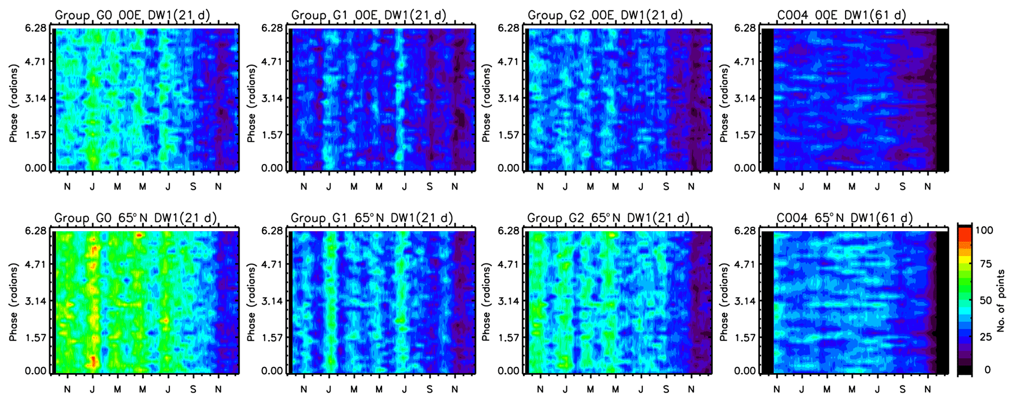
Figure 1Distribution of phase space for the tide DW1 from groups G0, G1 and G2 (±10 d data) as well as for the satellite C004 (±30 d data) during the study period (2009–2010) over the Equator and 65∘ N.
Data in each group (G0, G1, G2, C004) are investigated using the least-squares fitting technique. The following function is fit to the two-dimensional temperature data, T, at each altitude at universal time, t, and longitude, λ, to include (a) mean temperature variation (T0) as well as (b) diurnal (frequency, f1=1), semi-diurnal (f2=2) and ter-diurnal (f3=3) tides with wavenumbers sj ranging from −4 to 4; negative wavenumbers denote eastward-propagating tides, and positive wavenumbers denote westward-propagating tides and (c) SPWs with wavenumbers sk ranging from 1 to 3:
where Tij and ϕij are the amplitudes and phases of the tides, and Tk and ϕk are the amplitudes and phases of the SPWs. It may be noted that data from G0, G1 and G2 are analysed using ±10 d data, and data from C004 are analysed using ±30 d data. This equation results in 61 fitted parameters that are carefully investigated in the ensuing sections.
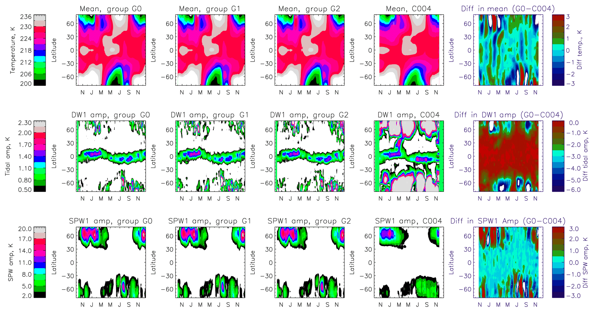
Figure 2Rows show the variation in mean temperature and the amplitudes of the DW1 tide and SPW1 wave, respectively. Columns are results from groups G0, G1 and G2, as well as from satellite C004, respectively, for 30 km of altitude. The last column is the numerical difference in results obtained from group G0 (±10 d data) and C004 (±30 d data).
The mean temperature and amplitudes of DW1 and SPW1 at 30 km obtained from the analysis of temperature data during November 2009–September 2010 are shown in Fig. 2. Each column indicates the results obtained from the three groups G0, G1 and G2 using ±10 d data and from satellite C004 using ±30 d data. The last column shows the numerical difference between the results obtained from group G0 and C004. It can be seen that the results obtained from the three groups are very similar, with extremely small differences over very fine scales. The variation in the mean temperature is similar in all groups. Over the Equator a semi-annual variation is observed (with maxima during November and May) along with an annual variation with a maximum during April–May and a minimum during November–December. Over middle and high latitudes a strong annual variation is observed with a maximum during summer and a minimum during winter. The sudden stratospheric warming (SSW) of 2010 is also observed in the Northern Hemisphere during January–February. The migrating diurnal tide, DW1, is very prominent at 30 km over the equatorial region with amplitudes in the range 1–1.5 K as a band-like structure around the Equator. The band is slightly shifted towards winter poles, i.e. northward during Northern Hemisphere winter and southward during Southern Hemisphere winter. Note that amplitudes below 0.5 K are not shown in the figure. At latitudes greater than 45∘ in the winter hemisphere, intermittent patches of DW1 are observed.
The amplitudes during January 2010 are enhanced relative to other times and in the range of 2–3 K. This coincides with the occurrence of the SSW of 2010. The SPW1 amplitudes are also large, reaching 18 K, over mid-latitudes above 45∘ in the winter hemisphere. The amplitude of this wave is stronger in the Northern Hemisphere than in the Southern Hemisphere. Furthermore, there is an apparent 60 d modulation in the amplitude of this wave. These plots show that similar results are obtained with all groups. Hence, for the rest of the paper only analysis from group G0 (that considers data from all six satellites) is discussed.
The results obtained using data over ±30 d from the single satellite, C004, are very different from the group results, particularly in the middle and high latitudes. The mean temperature is smoother over the 60 d period, and the difference between the mean temperature of group G0 and C004 (presented in the last column in Fig. 2) shows periodic variations of ∼60 d over the entire global region. The differences maximise during winter and spring in the high latitudes with magnitudes greater than 3 K. The amplitude of DW1 over the Equator and latitudes less than 30∘ is similar to those obtained from the analysis of the groups. However, the values are unusually large over middle and high latitudes, particularly over the regions poleward of 45∘. The differences show that DW1 amplitudes from C004 using ±30 d data are overestimated by more than 6 K, which is significant given that the maximum amplitude of DW1 (from the group analyses) in high latitudes is less than 3 K. The amplitude of SPW1 is, on the other hand, similar to the variation observed in the analysis of the data in groups. However, the former is smoothed over the time duration considered. Here, the difference panel in the last column shows that the SPW1 amplitude observed by data from C004 alone is also modulated by periodic variations of ∼60 d, particularly in the high-latitude winter atmosphere. These differences are of the order of ±3 K, which is small compared to the maximum SPW amplitudes.
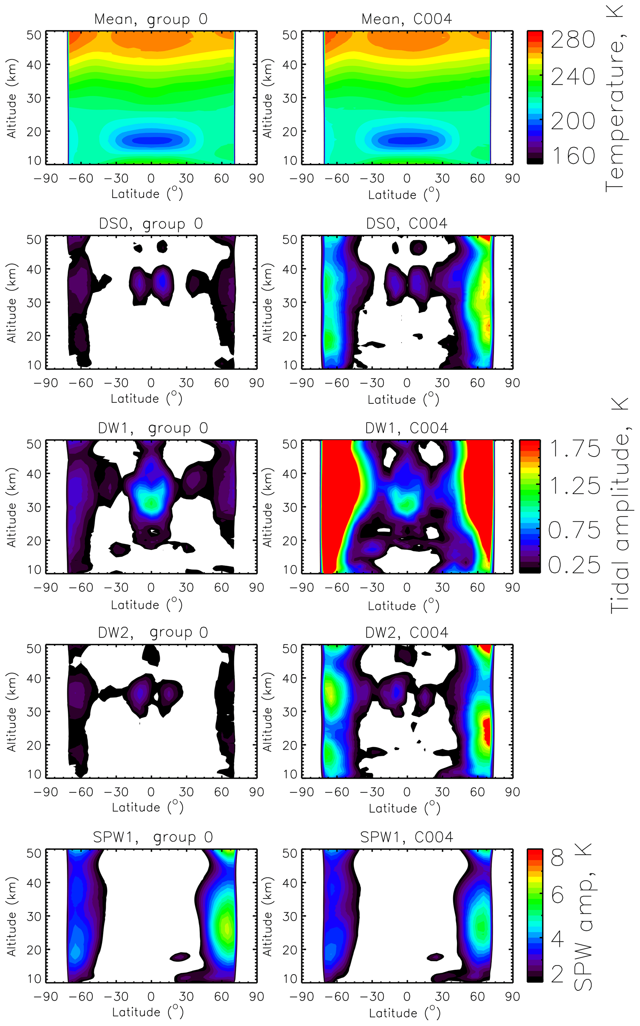
Figure 3Annual means of mean temperature (T0) and the amplitudes of diurnal tides (DS0, DW1, DW2) and a stationary planetary wave (SPW1) for group G0 and satellite C004 during 2010 (January–December). Note the overestimation of amplitudes of the migrating tide, particularly in middle and high latitudes in the analysis of data over ±30 d using a single satellite (C004).
Figure 3 shows the annual mean of the various wave parameters of interest in the current study using group G0 and satellite C004. The annual mean of the mean temperature is similar in both columns. However, the migrating diurnal tide and non-migrating tides are overestimated by C004 in the high latitudes. Over the Equator and low latitudes, the tidal amplitudes are similar. SPW1 amplitudes are marginally underestimated by C004 over high latitudes. This could be due to the effect of smoothing as more data were used in the analysis of the latter.
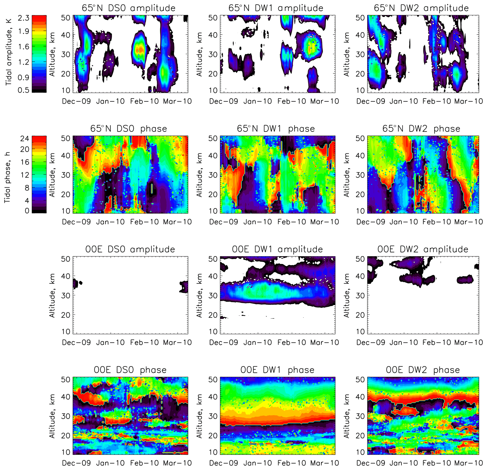
Figure 4Variation of the amplitudes and phases of DS0 (left column), DW1 (middle column) and DW2 (right column) during the winter of 2009–2010, i.e. from December 2009 to February 2010 over 65∘ N in the first and the second rows and the Equator in the third and fourth rows.
Figure 4 shows the variation of amplitudes and phases of DS0 (left column), DW1 (middle column) and DW2 (right column) during the winter of 2009–2010, i.e. from December 2009 to February 2010, over 65∘ N in the first and second rows and over the Equator in the third and fourth rows. These results are obtained from group G0. In the high-latitude winter hemisphere, DW1 shows large amplitudes of 2 K but only intermittently, and DS0 and DW2 also show similar intermittent behaviour in the range 1–2 K. The phase plots of these tides do not show any specific pattern as the waves themselves are intermittent. Over the Equator, the amplitude of DW1 maximises at 30 km and is in the range of 1–1.5 K. Its phase variation with altitude indicates that its wavelength is ∼25 km as is known from previous studies. Small amplitudes of 0.5 to 1 K are observed for DS0 and DW2 on either side of this equatorial band at 35 km. However, at all other altitudes over the Equator and low latitudes their amplitudes are zero (not shown here).
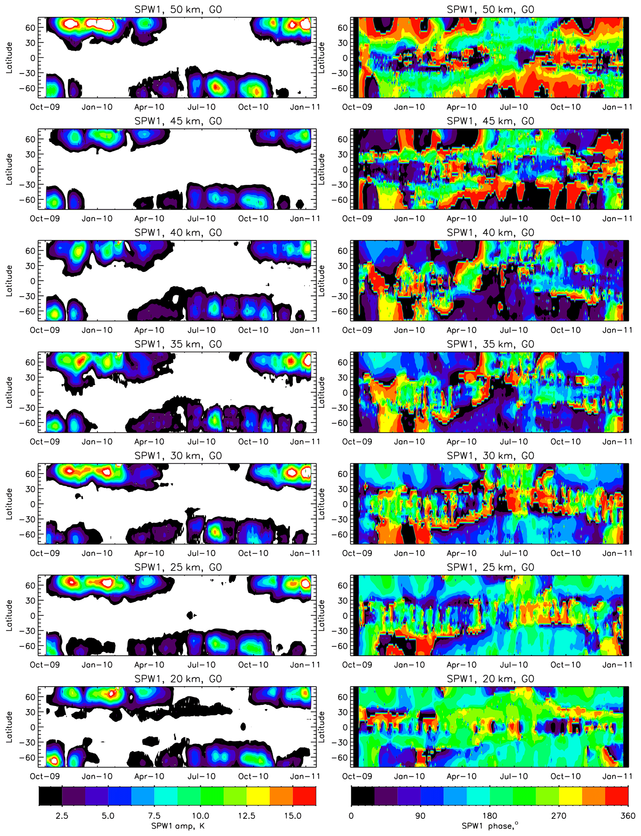
Figure 5Variation of the amplitude and phase of SPW1 at various altitudes from 20 to 50 km as a function of latitude and day of the year.
Figure 5 shows the variation of the amplitude and phase of SPW1 at various altitudes from 20 to 50 km (along the different rows) during the period of study. Large amplitudes of SPW1 are seen in the high-latitude winter atmosphere. The amplitudes of SPW1 over the Northern Hemisphere are largest during winter, with values reaching 18 K at 30 km of altitude. It is also seen that in January 2010, as the SSW started, the amplitude of SPW1 decreased to ∼6 K. In the Southern Hemisphere the amplitudes are smaller, with a maximum of ∼10 K at 30 km. Importantly, there is significant variability at a periodicity of ∼60 d at all altitudes, the modulation remaining coherent between both hemispheres. Investigation of the phase plots shows that the phase lines are nearly constant as a function of latitude at each height when large amplitudes of the SPWs are observed. The phase variation with altitude indicates that the vertical wavelength of SPW1 is in the range of 50 to 60 km at ∼60∘ N, and at ∼60∘ S.
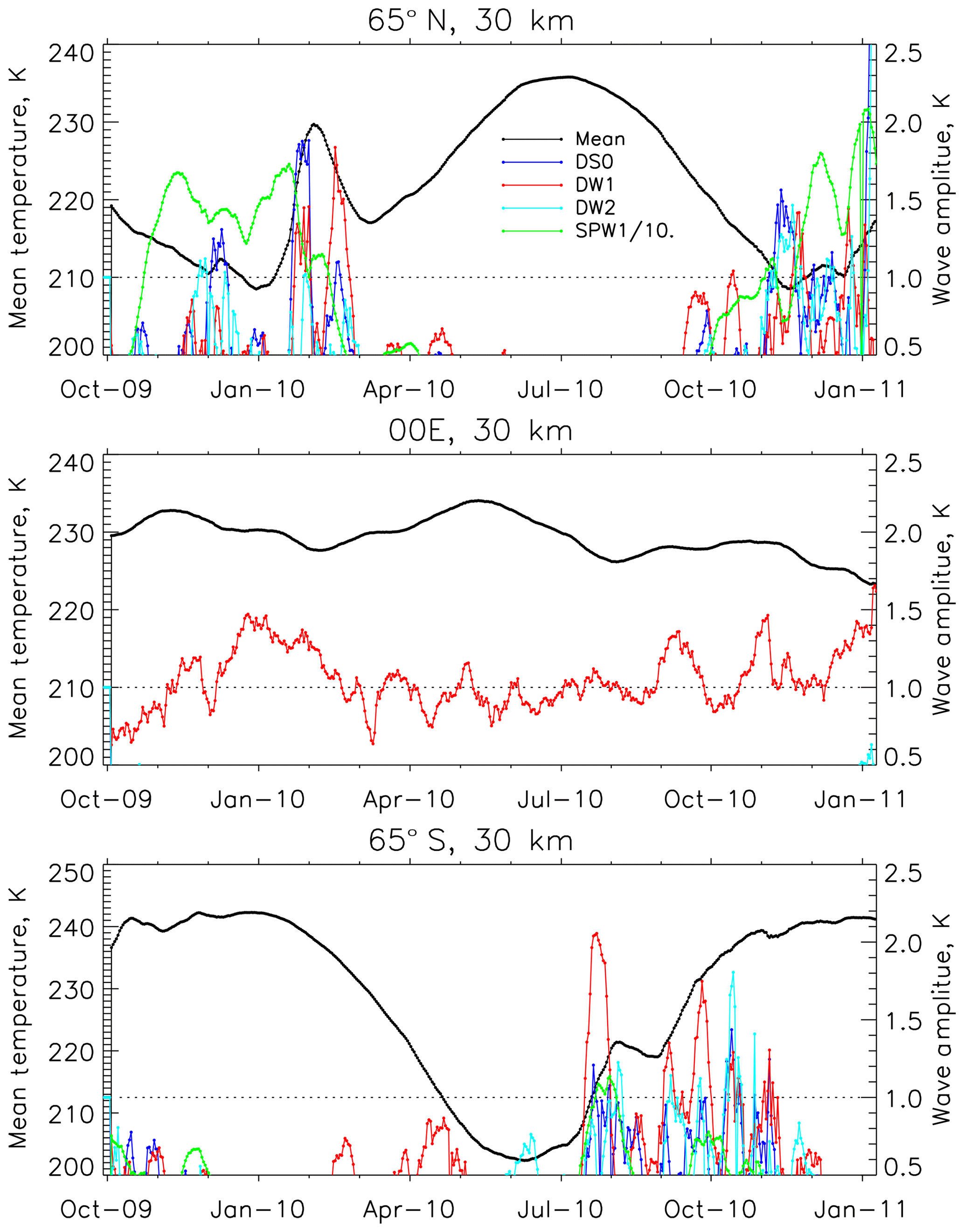
Figure 6Mean temperature (black) and the amplitudes of the DS0 (blue), DW1 (red), DW2 (cyan) and SPW1 (green) at 30 km at 65∘ N, the Equator and 65∘ S during the study period. The amplitude of SPW1 is scaled down by a factor of 10 for convenience.
Comparison of Figs. 4 and 5 shows that significant amplitudes of DS0 and DW2 occur at the same time as when SPW1 is strong. However, there does not seem to be any significant correlation between the non-migrating tides and the stationary planetary wave. To investigate this aspect further, Fig. 6 shows the mean temperature in black, amplitudes of the DS0 in blue, DW1 in red, DW2 in cyan and SPW1 in green at 30 km at 65∘ N, the Equator and 65∘ S. The amplitudes of the waves are indicated by the axis on the right of the figure with that of SPW1 scaled down by a factor of 10 for convenience. The most striking feature of the figure is the occurrence of the SSW in January 2010 at 65∘ N. Exactly during the time when the mean temperatures were increasing at a high rate, the amplitude of SPW was reduced drastically from 17 to 10 K, and the amplitudes of the three tides increased. The amplitude of DS0 is almost 2 K, that of DW1 is 1.5 K and that of DW2 is 1 K. Similar peaks are also observed after the event when the mean temperature is decreasing. At this point, the amplitude of DW1 maximises at 2 K, that of DS0 is 1 K and the amplitude of DW2 is less than 1 K. During summer there is no wave activity in either hemisphere. In the Southern Hemisphere at 65∘ S, tidal activity is observed as the temperatures start to rise in the winter. In particular, as the mean temperature increases rapidly during July 2010, the amplitude of DW1 maximises at ∼2 K and the amplitudes of DS0 and DW2 are of the order of 1 K. During the next 3–4 months, intermittent patches are observed when the amplitudes of DW1 and DW2 are ∼1.5 K. Over the Equator, on the other hand, the picture is very simple as there are no occurrences of significant amplitudes of DS0 and DW2. Interestingly, DW1 shows significant short-term variability at periodicities of the order of 30 d. If the data were analysed over 60 d intervals, this variability would not have been observed. The amplitudes of DW1 are marginally higher (∼1.5 K) during Northern Hemisphere winter and smaller (∼1 K) during summer.
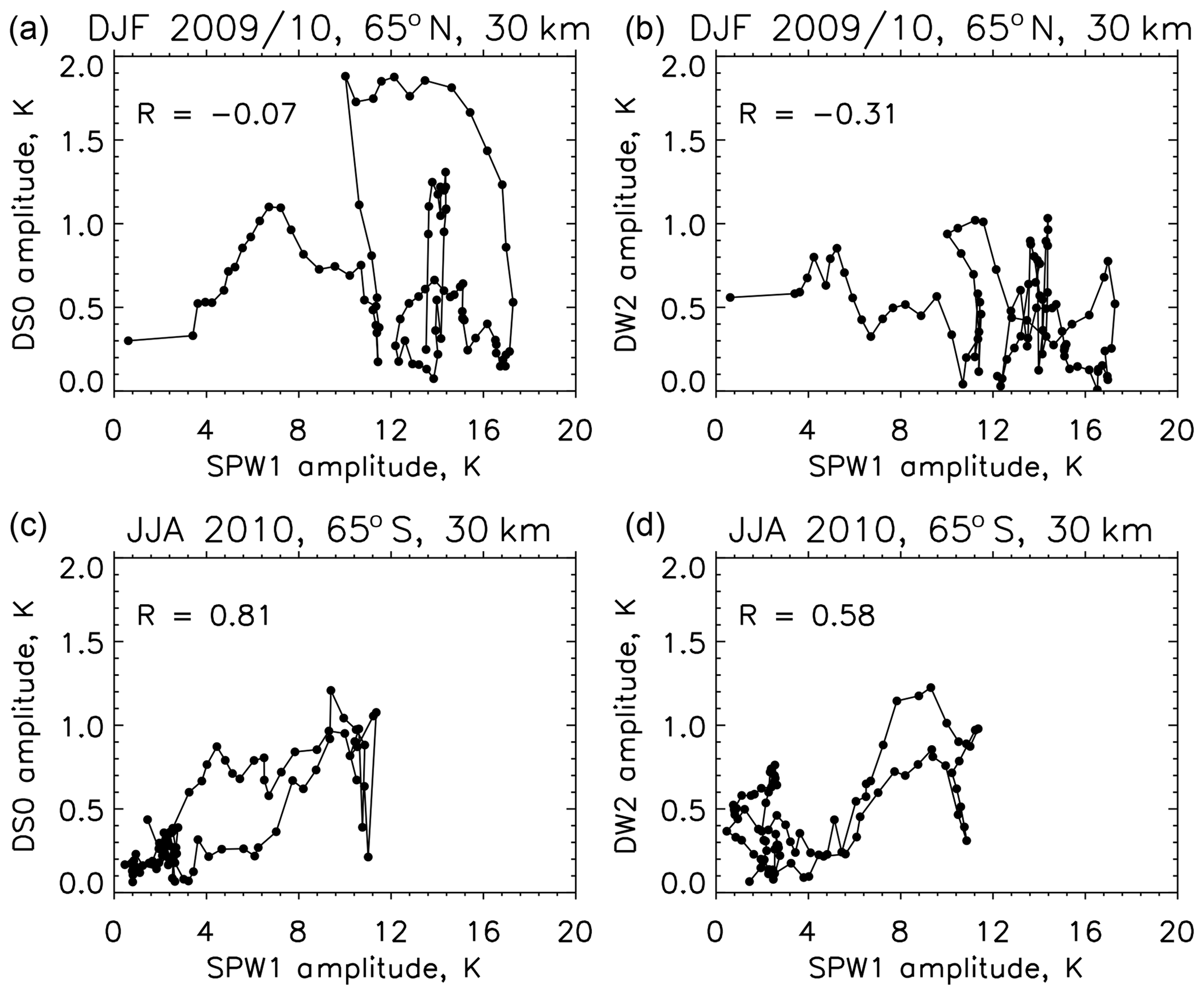
Figure 7Correlation between DS0 and SPW1 and between DW2 and SPW1 during winters at 65∘ latitude in the Northern and Southern Hemisphere.
To understand the simultaneous occurrence of non-migrating tides and stationary planetary waves, a simple correlation study is performed and is shown in Fig. 7. Panel (a) shows the correlation of DS0 and SPW1 at 65∘ N at 30 km for winter from December 2009 to February 2010. The correlation is negligible. Panel (b) shows the correlation between DW2 and SPW1 for the same latitude and altitude. Here the correlation is also not significant. Panels (c) and (d) show similar correlations for the Southern Hemisphere during June to August 2010, and there is good correlation between DS0 and SPW1 and a reasonable correlation between DW2 and SPW1. However, the amplitudes of the tides are all ∼1 K or smaller. Thus, no reasonable statistical relation can be established between the occurrence of non-migrating tides and stationary planetary waves.
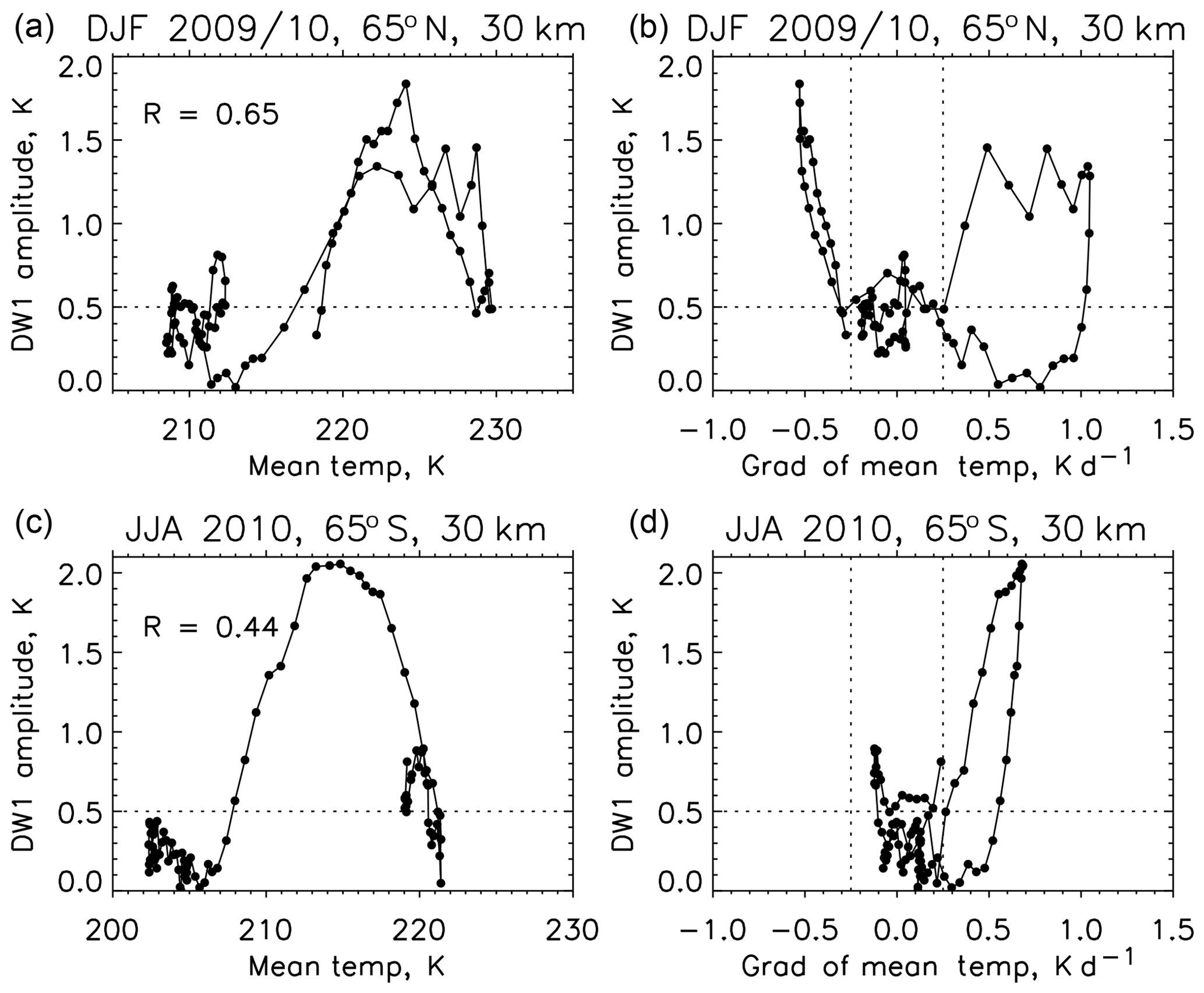
Figure 8Correlation between DW1 and mean temperature and between DW1 and the gradient in mean temperature during winters at 65∘ latitude in the Northern and Southern Hemisphere.
Figure 8 shows another correlation study between mean temperature and the DW1 tide. In panels (a) and (c) no significant correlation between the two parameters in either hemisphere is present. Panels (b) and (d) show the variation of DW1 as a function of gradient in the mean temperature. When the latter is larger than ±0.25 K d−1, the amplitudes of DW1 are also very large and increase with increasing gradient. The situation is same in the Southern Hemisphere. This is not observed when the gradients are smaller, and at these times the amplitudes of DW1 are smaller than 0.5 K and are negligible. This clearly indicates that there is an aliasing of energy into the DW1 tidal amplitude when the mean temperatures vary significantly.
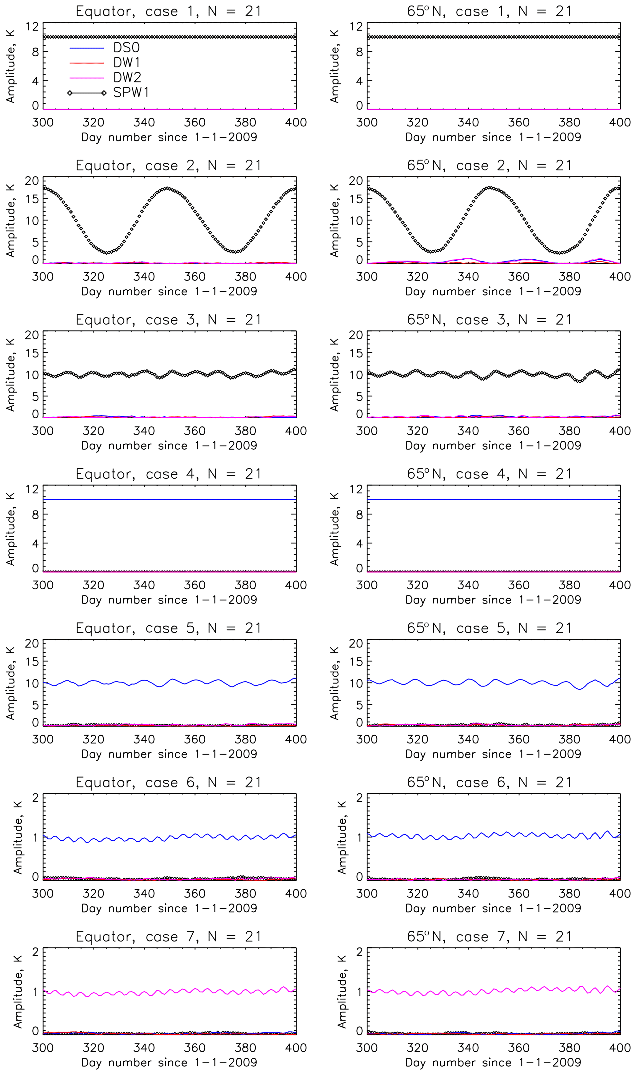
Figure 9Results of numerical experiments from cases 1 to 7 (Table 1) for atmospheres considered to have only one variability among SPW1, DS0 and DW2.
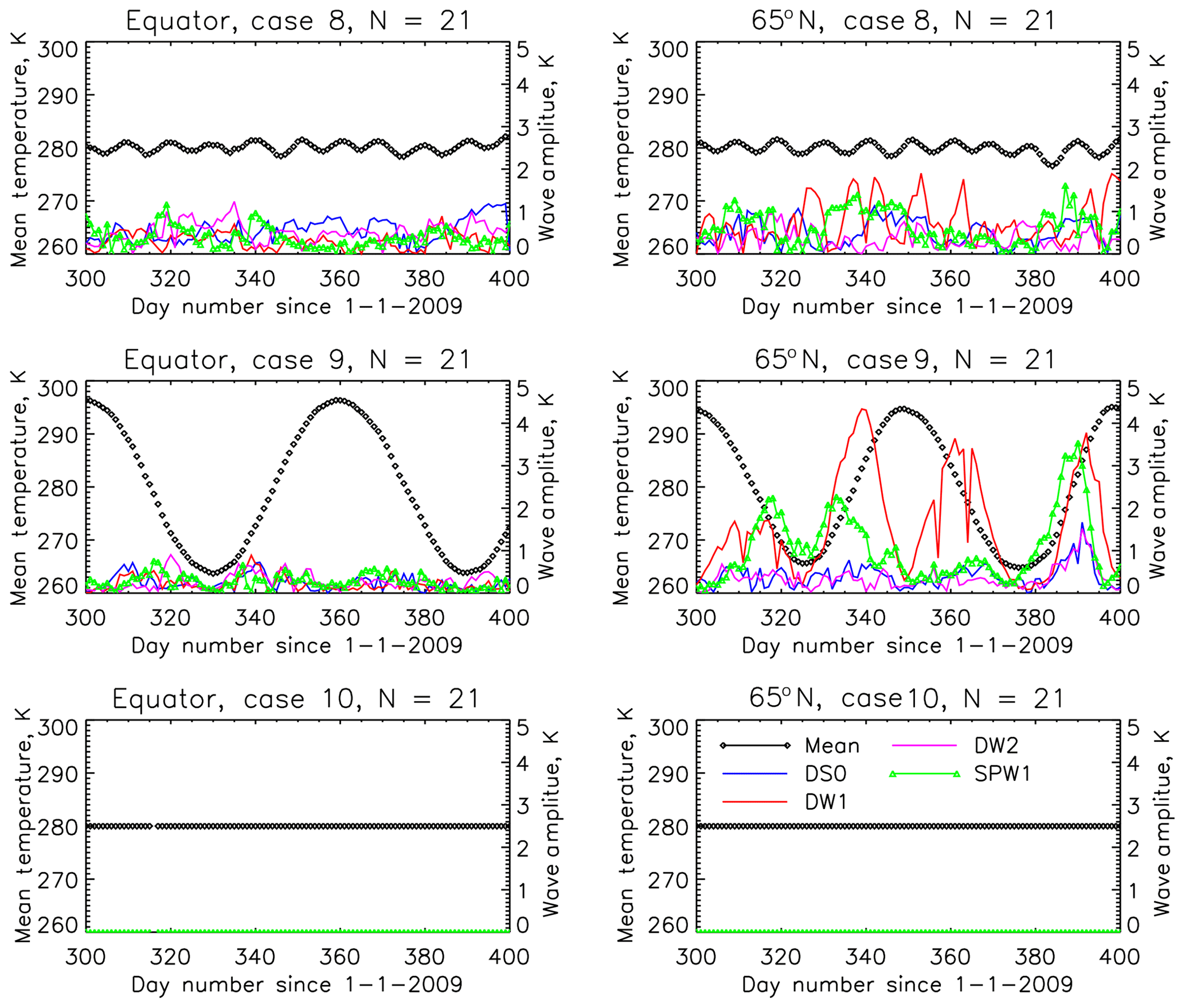
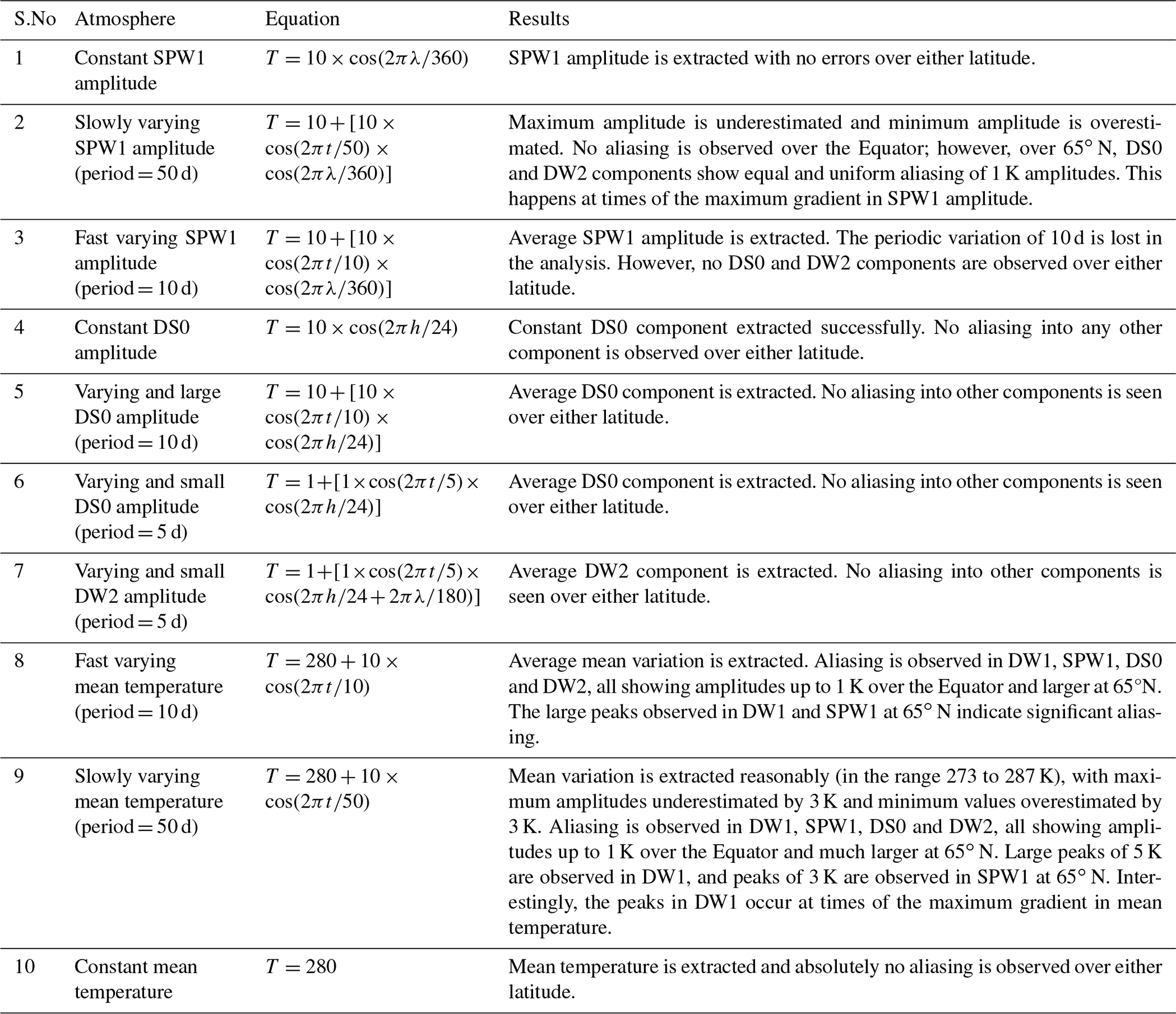
It was very clearly established that varying mean temperatures alias into the DW1 tide using SABER data (Sakazaki et al., 2012). However, in the case of COSMIC data, as the data sampling is irregular, it is difficult to establish such aliasing phenomena in the same way. To circumvent this problem, numerical experiments were performed to understand the extent to which aliasing occurs as a result of COSMIC data sampling. For the times and locations of COSMIC measurements over the Equator and at 65∘ N, a numerical atmosphere is created that consists of known variabilities. Table 1 describes the 10 cases considered for this study. The results from these numerical experiments are shown in Figs. 9 and 10 and are explained in detail in the table.
The extraction of tidal variability from satellite measurements with good accuracy and with no aliasing is a challenge. Using SABER temperature data, wave characteristics can be extracted over 60 d in the middle atmosphere. The amplitude of SPWs using SABER data are much smaller (Xu et al., 2014) than those obtained in the current study. During Northern Hemisphere winter, the maximum average amplitudes from SABER were 7.2±1.02 K at 45∘ N and 45 km. There was strong temporal correlation between the occurrence of SPWs and the non-migrating tides, which led to the conclusion that the latter were produced due to non-linear interactions of SPWs and migrating diurnal tides (Xu et al., 2014). The study by Xu et al. (2014) explicitly concentrated on the generation of these non-migrating tides and hence their conclusions. However, the current study shows that the amplitude of SPW1 is very large, of the order of 18 K, and the strong temporal correlation with DS0 and DW2 could also be caused due to aliasing of SPW1 into the non-migrating tides. In case 2 of the numerical experiments, it is observed that the aliasing of SPW1 into DS0 and DW2 is equal and uniform, and thus in the actual analysis if DS0 and DW2 are found to be equal and uniform, it is possible that the diagnosed variation in these tidal components might be due to aliasing. Thus, the question of whether non-linear interactions between SPW1 and DW1 produce DS0 and DW2 is still debatable. Although non-linear interactions cannot be entirely ruled out, the current study shows that the contribution of this mechanism to producing non-migrating tides in the middle- and high-latitude stratosphere is not as important as indicated by earlier studies that are particularly dependent on the analysis of SABER data (Xu et al., 2014). The current study indicates that the DS0 and DW2 components are much smaller than those observed earlier using SABER data.
Baumgarten and Stober (2019) derived short-term tidal variability in the altitude range from 30 to 70 km using temperature derived from lidar observations at Kühlungsborn (54∘ N, 12∘ E), a mid-latitude station. The diurnal tide (including all wavenumbers) in temperature and winds was extracted from lidar data and compared with the DW1 component of temperature and winds from the Modern-Era Retrospective analysis for Research and Applications Version 2 (MERRA-2). It was shown that the local tidal fields are dominated by the migrating diurnal and migrating semi-diurnal tides and that other components are negligible. This indicates that the non-migrating components make a small contribution to net tidal fields and thus supports the conclusions of the current study that diagnosed non-migrating tidal signatures could possibly be due to aliasing. Aliasing problems involved in SABER data are difficult to verify due to a lack of similar global observations, but comparisons have been made with models and reanalysis and it was noted that there are significant inconsistencies in the tidal signatures determined from the various sources (Sakazaki et al., 2018). It was found that the amplitude of the trapped diurnal migrating tide in the upper stratosphere is significantly smaller in reanalyses than that in SABER. The current study also indicates that SABER tidal amplitudes are overestimated, particularly in the middle and high latitudes. Results from a space–time spectral analysis of gridded monthly COSMIC data for the period from 2007 to 2008 also show that the DW1 peaks at 30 km over the equatorial latitudes (Pirscher et al., 2010). It was shown in the paper by Pirscher et al. (2010) that sampling was insufficient northward of 50∘, and the spectral amplitude associated with the sampling error was large. However, in the current study (wherein a different time interval and hence a different distribution of satellite observations were selected) the wave phase space is sufficiently well sampled (Fig. 1). By using the least-squares method over shorter lengths of data, it was possible to extract the different wave components. The numerical experiments show that with the given sampling and the technique used, it can be verified whether the extracted spectral components SPW1, DS0, DW1 and DW2 are geophysical or are a result of aliasing.
There are also studies that have shown that the time evolution of DW2 over the equatorial mesopause region follows SPW1 variations in the high-latitude stratosphere (Lieberman et al., 2015; Niu et al., 2018). It is proposed that middle- to high-latitude stratospheric SPWs are ducted upward and equatorward, interact with equatorial DW1 over the mesopause, and thereby generate DW2 over the equatorial mesopause region. DS0 is not discussed by Lieberman et al. (2015). Niu et al. (2018) investigated the SPW1–DW1 interaction during SSWs using the extended Canadian Middle Atmosphere Model (eCMAM) data and found good but varying degrees of correlation with DS0 and DW2 during 20 out of 31 SSW events, indicating that the strength of non-linear interactions also varied from year to year. As the correlations are not observed during all SSW events, the proposed mechanism of non-linear interactions is still unproven.
In the current study, during the SSW of 2010, the peaks observed in DW1, DS0 and DW2 are most likely due to aliasing. At 65∘ N, as the temperature increases (decreases) steeply during the onset (decay) of the warming episode, the DW1 component is observed to be large (1.5 to 2 K). The entire SSW event lasted ∼60 d, and the temporal evolution of its fields is very similar to the numerical experiment in case 9, in which significant aliasing into DW1 is observed. This experiment indicates that over high latitudes, when there is a large gradient in the mean temperature, peaks of large amplitude in DW1 are observed, which are not geophysical in nature. At the same time, the SPW1 component steeply decreased during the onset of the episode, from which the DS0 and DW2 components may have arisen due to aliasing. In addition, there is aliasing into SPW1 of the order of 2–3 K, but since the observed SPW1 amplitudes are much larger (18 K), this is of less geophysical significance. The amplitude of 2 K in DS0 during the onset of the event may have some geophysical significance, but further investigation is needed before this is clear.
McCormack et al. (2017) investigated the short-term tidal variability during the SSWs of January 2010 and January 2013 using high-altitude Navy Global Environmental Model (NAVGEM) data in the mesosphere and lower thermosphere region. NAVGEM is the result of the assimilation of middle atmospheric data from nine meteor radar stations and other satellite instruments, including SABER onboard the TIMED satellite. The results show a reduction in the semi-diurnal amplitude before the onset of the SSW and an increase after the event, peaking 10–14 d later. Short-term tidal variability has also been deduced using data from a sodium lidar as well as simultaneous SABER retrievals and TIME-GCM results in the mesosphere and lower thermosphere (Liu et al., 2007). Liu et al. (2007) found large tidal variability which could be the result of interactions with planetary waves. The migrating diurnal tidal amplitude was modulated by the planetary wave of 5–7 d period. Such interactions are worth studying in the future using COSMIC data by considering travelling planetary waves to obtain more insights into the tidal variability. Unfortunately, the altitude coverage of COSMIC is only up to the stratopause, and thus tidal characteristics cannot be extracted for altitudes above 45 to 50 km. However, the current study clearly establishes the fact that with COSMIC data short-term tidal variability can be obtained in combination with a consideration of the aliasing involved. The following may thus be concluded from the current study.
-
COSMIC data are better suited for tidal studies than along-track observations from a single satellite due to better phase sampling of tides and waves; however, due to the lack of altitude coverage the studies are confined to the lower stratosphere.
-
The migrating diurnal tide (DW1) is found to maximise at 30 km over the Equator; its seasonal variation in latitude is attributed to the excitation of more than one tidal mode in the troposphere. The vertical wavelength is of the order of 25 km.
-
A stationary planetary wave of wavenumber 1 (SPW1) peaks in the winter hemisphere over high latitudes with a vertical wavelength of 50–60 km at 65∘ N. It exhibits a strong ∼60 d variability which was not observed earlier in SABER studies.
-
DS0 and DW2 components are relatively small and only present intermittently in the high-latitude middle atmosphere COSMIC analysis. Most of the peaks seem to be appearing due to aliasing.
-
Aliasing is significantly reduced when data are analysed over ±10 d using COSMIC data. However, it still exists, and the numerical experiments performed in the current study show that DS0 and DW2 components arise when there is a rapid change in the SPW1 amplitude over time. Similar aliasing into the DW1 component is prominently observed when there is a rapid change in the mean temperature, particularly in the high latitudes.
-
These exercises indicate that at the time of the SSW in January 2010, the peaks observed in DW1, as well as DS0 and DW2, are likely a manifestation of the aliasing effects involved in satellite data analysis and that they may not be geophysical. Analyses of satellite data need to be done extremely carefully when identifying the various tidal components and their characteristics.
It is thus concluded that non-linear interactions are not a very important source for the generation of non-migrating tides in the winter high-latitude stratosphere.
The codes are prepared in IDL and can be supplied on request.
The data used in the current study are obtained from UCAR/COSMIC https://cdaac-www.cosmic.ucar.edu/ (COSMIC Data Analysis and Archive Center, 2013). The data are freely available.
The supplement related to this article is available online at: https://doi.org/10.5194/angeo-38-421-2020-supplement.
UD and WEW conceived the idea. UD performed the data analysis. CJP provided insights into the usage of COSMIC data. WEW designed and SKD performed the numerical experiments. UD and WEW analysed and finalised the results after discussion with all authors. UD prepared the paper with contributions from all authors.
The authors declare that they have no conflict of interest.
The authors acknowledge the UCAR/COSMIC programme for providing free access to FORMOSAT-3/COSMIC “atmPrf” temperature data. Uma Das is supported by Early Career Research Award ECR/2017/002258 by the Science and Engineering Research Board (SERB), Government of India. Support for portions of this work came from the National Science and Engineering Research Council (NSERC) Collaborative Research and Training Experience Grant (384996-2010) for CANDAC activities. WEW was supported by an NSERC Discovery Grant. Chen Jeih Pan is supported by the Ministry of Science and Technology of Taiwan through the grant MOST-107-2111-M-008-006.
This research has been supported by the Science and Engineering Board (SERB), Government of India (grant no. ECR/2017/002258), the Ministry of Science and Technology of Taiwan (grant no. MOST-107-2111-M-008-006), and the National Science and Engineering Research Council (NSERC) Collaborative Research and Training Experience Grant (384996-2010) for CANDAC activities.
This paper was edited by Gunter Stober and reviewed by two anonymous referees.
Anthes, R. A., Ector, D., Hunt, D. C., Kuo, Y. H., Rocken, C., Schreiner, W. S., Sokolovskiy, S. V., Syndergaard, S., Wee, T. K., Zeng, Z., Bernhardt, P. A., Dymond, K. F., Chen, Y., Liu, H., Manning, K., Randel, W. J., Trenberth, K. E., Cucurull, L., Healy, S. B., Ho, S. P., McCormick, C., Meehan, T. K., Thompson, D. C., and Yen, N. L.: The COSMIC/FORMOSAT-3 Mission: Early Results, Bull. Am. Meteorl. Soc., 89, 313–333, 2008. a, b
Baumgarten, K. and Stober, G.: On the evaluation of the phase relation between temperature and wind tides based on ground-based measurements and reanalysis data in the middle atmosphere, Ann. Geophys., 37, 581–602, https://doi.org/10.5194/angeo-37-581-2019, 2019. a, b, c
Baumgarten, K., Gerding, M., Baumgarten, G., and Lubken, F.-J.: Temporal variability of tidal and gravity waves during a record long 10-day continuous lidar sounding, Atmos. Chem. Phys., 18, 371–384, https://doi.org/10.5194/acp-18-371-2018, 2018. a
Chapman, S. and Lindzen, R.: Atmospheric Tides: Thermal and Gravitational, Springer Netherlands, https://doi.org/10.1007/978-94-010-3399-2, 1970. a
COSMIC Data Analysis and Archive Center (Constellation Observing System for Meteorology/Ionosphere and Climate): Atmospheric Profiles (atmPrf) from COSMIC Occultation Data. COSMIC Data Analysis and Archive Center, https://cdaac-www.cosmic.ucar.edu/cdaac/products.html (last access: 6 August 2019), 2013.
Das, U. and Pan, C. J.: Validation of FORMOSAT-3/COSMIC level 2 “atmPrf” global temperature data in the stratosphere, Atmos. Meas. Tech., 7, 731–742, https://doi.org/10.5194/amt-7-731-2014, 2014. a, b
Forbes, J., Kilpatrick, M., Fritts, D., Manson, A., and Vincent, R.: Zonal mean and tidal dynamics from space: An empirical examination of aliasing and sampling issues, Springer, Ann. Geophys., 15, 1158–1164, 1997. a
Forbes, J. M. and Garrett, H. B.: Theoretical Studies of Atmospheric Tides, Rev. Geophys. Space Phys., 17, 1951–1981, 1979. a
Gan, Q., Du, J., Ward, W. E., Beagley, S. R., Fomichev, V. I., and Zhang, S.: Climatology of the diurnal tides from eCMAM30 (1979 to 2010) and its comparison with SABER, Earth, Planet. Space, 66, 1–24, 2014. a
Hagan, M. E. and Forbes, J. M.: Migrating and nonmigrating diurnal tides in the middle and upper atmosphere excited by tropospheric latent heat release, J. Geophys. Res., 107, 4754, https://doi.org/10.1029/2001JD001236, 2002. a
Hagan, M. E. and Forbes, J. M.: Migrating and nonmigrating semidiurnal tides in the upper atmosphere excited by tropospheric latent heat release, J. Geophys. Res., 108, 1062, https://doi.org/10.1029/2002JA009466, 2003. a
Immel, T., Sagawa, E., England, S., Henderson, S., Hagan, M., Mende, S., Frey, H., Swenson, C., and Paxton, L.: Control of equatorial ionospheric morphology by atmospheric tides, Geophys. Res. Lett., 33, L15108, https://doi.org/10.1029/2006GL026161, 2006. a
Kuo, Y.-H., Wee, T.-K., Sokolovskiy, S., Rocken, C., Schreiner, W., Hunt, D., and Anthes, R.: Inversion and Error Estimation of GPS Radio Occultation Data, J. Met. Soc. Jpn., 82, 507–531, 2004. a, b
Kursinski, E. R., Hajj, G. A., Schofield, J. T., Linfield, R. P., and Hardy, K. R.: Observing Earth's atmosphere with radio occultation measurements using the Global Positioning System, J. Geophys. Res., 102, 23429–23465, https://doi.org/10.1029/97JD01569, 1997. a, b, c
Lieberman, R., Riggin, D., Ortland, D., Oberheide, J., and Siskind, D.: Global observations and modeling of nonmigrating diurnal tides generated by tide-planetary wave interactions, J. Geophys. Res.-Atmos., 120, 11–419, 2015. a, b
Liu, H.-L., Li, T., She, C.-Y., Oberheide, J., Wu, Q., Hagan, M., Xu, J., Roble, R., Mlynczak, M., and Russell III, J.: Comparative study of short-term diurnal tidal variability, J. Geophys. Res.-Atmos., 112, D18108, https://doi.org/10.1029/2007JD008542, 2007. a, b, c
McCormack, J., Hoppel, K., Kuhl, D., de Wit, R., Stober, G., Espy, P., Baker, N., Brown, P., Fritts, D., Jacobi, C., Janches, D., Mitchekk, N., Ruston, B., Swadley, S., Viner, K., and Whitcomb, T.: Comparison of mesospheric winds from a high-altitude meteorological analysis system and meteor radar observations during the boreal winters of 2009–2010 and 2012–2013, J. Atmos. Sol.-Terr. Phys., 154, 132–166, 2017. a, b, c
Mertens, C. J., Schmidlin, F. J., Goldberg, R. A., Remsberg, E. E., Pesnell, W. D., Russell III, J. M., Mlynczak, M. G., López-Puertas, M., Wintersteiner, P. P., Picard, R. H., Winick, J. R., and Gordley, L. L.: SABER observations of mesospheric temperatures and comparisons with falling sphere measurements taken during the 2002 summer MaCWAVE campaign, Geophys. Res. Lett., 31, L03105, https://doi.org/10.1029/2003GL018605, 2004. a
Mukhtarov, P., Pancheva, D., and Andonov, B.: Global structure and seasonal and interannual variability of the migrating diurnal tide seen in the SABER/TIMED temperatures between 20 and 120 km, J. Geophys. Res., 114, A02309, https://doi.org/10.1029/2008JA013759, 2009. a
Niu, X., Du, J., and Zhu, X.: Statistics on Nonmigrating Diurnal Tides Generated by Tide-Planetary Wave Interaction and Their Relationship to Sudden Stratospheric Warming, Atmosphere, 9, 416, https://doi.org/10.3390/atmos9110416, 2018. a, b
Oberheide, J., Hagan, M., Roble, R., and Offermann, D.: Sources of nonmigrating tides in the tropical middle atmosphere, J. Geophys. Res.-Atmos., 107, 4567, https://doi.org/10.1029/2002JD002220, 2002. a
Oberheide, J., Forbes, J. M., Zhang, X., and Bruinsma, S. L.: Wave-driven variability in the ionosphere-thermosphere-mesosphere system from TIMED observations: What contributes to the “wave 4”?, J. Geophys. Res., 116, A01306, https://doi.org/10.1029/2010JA015911, 2011a. a
Oberheide, J., Forbes, J. M., Zhang, X., and Bruinsma, S. L.: Climatology of upward propagating diurnal and semidiurnal tides in the thermosphere, J. Geophys. Res., 116, A11306, https://doi.org/10.1029/2011JA016784, 2011b. a
Pancheva, D. and Mukhtarov, P.: Wavelet analysis on transient behaviour of tidal amplitude fluctuations observed by meteor radar in the lower thermosphere above Bulgaria, Ann. Geophys., 18, 316–331, https://doi.org/10.1007/s00585-000-0316-3, 2000. a
Pedatella, N., Oberheide, J., Sutton, E., Liu, H.-L., Anderson, J., and Raeder, K.: Short-term nonmigrating tide variability in the mesosphere, thermosphere, and ionosphere, J. Geophys. Res.-Space, 121, 3621–3633, 2016. a
Pirscher, B., Foelsche, U., Borsche, M., Kirchengast, G., and Kuo, Y. H.: Analysis of migrating diurnal tides detected in FORMOSAT-3/COSMIC temperature data, J. Geophys. Res., 115, D14108, https://doi.org/10.1029/2009JD013008, 2010. a, b, c
Remsberg, E., Lingenfelser, G., Harvey, V. L., Grose, W., Russell, J., I., Mlynczak, M., Gordley, L., and Marshall, B. T.: On the verification of the quality of SABER temperature, geopotential height, and wind fields by comparison with Met Office assimilated analyses, J. Geophys. Res., 108, 4628, https://doi.org/10.1029/2003JD003720, 2003. a
Remsberg, E. E., Marshall, B. T., Garcia-Comas, M., Krueger, D., Lingenfelser, G. S., Martin-Torres, J., Mlynczak, M. G., Russell, J. M., Smith, A. K., Zhao, Y., Brown, C., Gordley, L. L., Lopez-Gonzalez, M. J., Lopez-Puertas, M., She, C. Y., Taylor, M. J., and Thompson, R. E.: Assessment of the quality of the Version 1.07 temperature-versus-pressure profiles of the middle atmosphere from TIMED/SABER, J. Geophys. Res., 113, D17101, https://doi.org/10.1029/2008JD010013, 2008. a, b
Sakazaki, T., Fujiwara, M., Zhang, X., Hagan, M. E., and Forbes, J. M.: Diurnal tides from the troposphere to the lower mesosphere as deduced from TIMED/SABER satellite data and six global reanalysis data sets, J. Geophys. Res.-Atmos., 117, D13108, https://doi.org/10.1029/2011jd017117, 2012. a, b, c
Sakazaki, T., Fujiwara, M., and Shiotani, M.: Representation of solar tides in the stratosphere and lower mesosphere in state-of-the-art reanalyses and in satellite observations, Atmos. Chem. Phys., 18, 1437–1456, https://doi.org/10.5194/acp-18-1437-2018, 2018. a, b
Scherllin-Pirscher, B., Steiner, A. K., Kirchengast, G., Schwärz, M., and Leroy, S. S.: The power of vertical geolocation of atmospheric profiles from GNSS radio occultation, J. Geophys. Res.-Atmos., 122, 1595–1616, 2017. a
She, C. Y., Li, T., Collins, R. L., Yuan, T., Williams, B. P., Kawahara, T. D., Vance, J. D., Acott, P., Krueger, D. A., Liu, H.-L., and Hagan, M. E.: Tidal perturbations and variability in the mesopause region over Fort Collins, CO (41∘ N, 105∘ W): Continuous multi-day temperature and wind lidar observations, Geophys. Res. Lett., 31, L24111, https://doi.org/10.1029/2004GL021165, 2004. a, b
Shepherd, G. G., Thuillier, G., Cho, Y. M., Duboin, M. L., Evans, W. F. J., Gault, W. A., Hersom, C., Kendall, D. J. W., Lathuillère, C., Lowe, R. P., McDade, I. C., Rochon, Y. J., Shepherd, M. G., Solheim, B. H., Wang, D. Y., and Ward, W. E.: The Wind Imaging Interferometer (WINDII) on the Upper Atmosphere Research Satellite: A 20 year perspective, Rev. Geophys., 50, RG2007, https://doi.org/10.1029/2012RG000390, 2012. a
Wu, D. L. and Jiang, J. H.: Interannual and seasonal variations of diurnal tide, gravity wave, ozone, and water vapor as observed by MLS during 1991–1994, Adv. Space Res., 35, 1999–2004, 2005. a
Wu, D. L., McLandress, C., Read, W. G., Waters, J. W., and Froidevaux, L.: Equatorial diurnal variations observed in UARS Microwave Limb Sounder temperature during 1991-1994 and simulated by the Canadian Middle Atmosphere Model, J. Geophys. Res.-Atmos., 103, 8909–8917, 1998. a
Wu, Q., Killeen, T. L., Ortland, D. A., Solomon, S. C., Gablehouse, R. D., Johnson, R. M., Skinner, W. R., Niciejewski, R. J., and Franke, S. J.: TIMED Doppler interferometer (TIDI) observations of migrating diurnal and semidiurnal tides, J. Atmos. Sol.-Terr. Phys., 68, 408–417, 2006. a
Wu, Q., McEwen, D., Guo, W., Niciejewski, R., Roble, R., and Won, Y.-I.: Long-term thermospheric neutral wind observations over the northern polar cap, J. Atmos. Sol.-Terr. Phys., 70, 2014–2030, 2008. a
Xu, J., Smith, A. K., Liu, M., Liu, X., Gao, H., Jiang, G., and Yuan, W.: Evidence for nonmigrating tides produced by the interaction between tides and stationary planetary waves in the stratosphere and lower mesosphere, J. Geophys. Res., 119, 471–489, https://doi.org/10.1002/2013jd020150, 2014. a, b, c, d, e, f
Xue, X., Wan, W., Xiong, J., and Dou, X.: Diurnal tides in mesosphere/low-thermosphere during 2002 at Wuhan (30.6∘ N, 114.4∘ E) using canonical correlation analysis, J. Geophys. Res., 112, D06104, https://doi.org/10.1029/2006JD007490, 2007. a
Zeng, Z., Randel, W., Sokolovskiy, S., Deser, C., Kuo, Y.-H., Hagan, M., Du, J., and Ward, W.: Detection of migrating diurnal tide in the tropical upper troposphere and lower stratosphere using the Challenging Minisatellite Payload radio occultation data, J. Geophys. Res.-Atmos., 113, D03102, https://doi.org/10.1029/2007JD008725, 2008. a
Zhang, X., Forbes, J. M., Hagan, M. E., Russell, J. M., Palo, S. E., Mertens, C. J., and Mlynczak, M. G.: Monthly tidal temperatures 20–120 km from TIMED/SABER, J. Geophys. Res., 111, A10S08, https://doi.org/10.1029/2005JA011504, 2006. a