Model of the propagation of very low-frequency beams in the Earth–ionosphere waveguide: principles of the tensor impedance method in multi-layered gyrotropic waveguides

The modeling of very low-frequency (VLF) electromagnetic (EM) beam propagation in the Earth–ionosphere waveguide (WGEI) is considered. A new tensor impedance method for modeling the propagation of electromagnetic beams in a multi-layered and inhomogeneous waveguide is presented. The waveguide is assumed to possess the gyrotropy and inhomogeneity with a thick cover layer placed above the waveguide. The influence of geomagnetic field inclination and carrier beam frequency on the characteristics of the polarization transformation in the Earth–ionosphere waveguide is determined. The new method for modeling the propagation of electromagnetic beams allows us to study the (i) propagation of the very low-frequency modes in the Earth–ionosphere waveguide and, in perspective, their excitation by the typical Earth–ionosphere waveguide sources, such as radio wave transmitters and lightning discharges, and (ii) leakage of Earth–ionosphere waveguide waves into the upper ionosphere and magnetosphere. The proposed approach can be applied to the variety of problems related to the analysis of the propagation of electromagnetic waves in layered gyrotropic and anisotropic active media in a wide frequency range, e.g., from the Earth–ionosphere waveguide to the optical waveband, for artificial signal propagation such as metamaterial microwave or optical waveguides.

1 Introduction

The results of the analytical and numerical study of very low-frequency (VLF) electromagnetic (EM) wave/beam propagation in the lithosphere–atmosphere–ionosphere–magnetosphere system (LAIM), in particular in the Earth–ionosphere waveguide (WGEI), are presented. The amplitude and phase of the VLF wave propagates in the Earth–ionosphere waveguide can change, and these changes may be observable using ground-based and/or satellite detectors. This reflects the variations in ionospheric electrodynamic characteristics (complex dielectric permittivity) and the influences on the ionosphere, for example, “from above” by the Sun–solar-wind–magnetosphere–ionosphere chain (Patra et al., 2011; Koskinen, 2011; Boudjada et al., 2012; Wu et al., 2016; Yiğit et al., 2016). Then the influence on the ionosphere “from below” comes from the most powerful meteorological, seismogenic and other sources in the lower atmosphere and lithosphere and Earth, such as cyclones and hurricanes (Nina et al., 2017; Rozhnoi et al., 2014; Chou et al., 2017) as well as from earthquakes (Hayakawa, 2015; Surkov and Hayakawa, 2014; Sanchez-Dulcet et al., 2015) and tsunamis. From inside the ionosphere, strong thunderstorms, lightning discharges, and terrestrial gamma-ray flashes or sprite streamers (Cummer et al., 1998; Qin et al., 2012; Dwyer, 2012; Dwyer and Uman, 2014; Cummer et al., 2014; Mezentsev et al., 2018) influence the ionospheric electrodynamic characteristics as well. Note that the VLF signals are very important for the merging of atmospheric physics and space plasma physics with astrophysics and high-energy physics. The corresponding “intersection area” for these four disciplines includes cosmic rays and currently very popular objects of investigation – high-altitude discharges (sprites), anomalous X-ray bursts and powerful gamma-ray bursts. The key phenomena for the occurrence of all of these objects is the appearance of the runaway avalanche in the presence of high-energy seed electrons. In the atmosphere, there are cosmic-ray secondary electrons (Gurevich and Zybin, 2001). Consequently, these phenomena are intensified during the air shower generating by cosmic particles (Gurevich and Zybin, 2001; Gurevich et al., 2009). The runaway breakdown and lightning discharges including high-altitude ones can cause radio emission both in the high-frequency (HF) range, which could be observed using the Low-Frequency Array (LOFAR) radio telescope network facility and other radio telescopes (Buitink et al., 2014; Scholten et al., 2017; Hare et al., 2018), and in the VLF range (Gurevich and Zybin, 2001). The corresponding experimental research includes the measurements of the VLF characteristics by the international measurement system of the “transmitted-receiver” pairs separated by a distance of a couple thousand kilometers (Biagi et al., 2011, 2015). The World Wide Lightning Location Network is one of the international facilities for VLF measurements during thunderstorms with lightning discharges (Lu et al., 2019). Intensification of magnetospheric research, wave processes, particle distribution and wave–particle interaction in the magnetosphere including radiation belts leads to the great interest in VLF plasma waves, in particular whistlers (Artemyev et al., 2013, 2015; Agapitov et al., 2014, 2018).

The differences of the proposed model for the simulation of VLF waves in the WGEI from others can be summarized in three main points. (i) In distinction to the impedance invariant imbedding model (Shalashov and Gospodchikov, 2011; Kim and Kim, 2016), our model provides an optimal balance between the analytical and numerical approaches. It combines analytical and numerical approaches based on the matrix sweep method (Samarskii, 2001). As a result, this model allows for analytically obtaining the tensor impedance and, at the same time, provides high effectiveness and stability for modeling. (ii) In distinction to the full-wave finite-difference time domain models (Chevalier and Inan, 2006; Marshall and Wallace, 2017; Yu et al., 2012; Azadifar et al., 2017), our method provides the physically clear lower and upper boundary conditions, in particular physically justified upper boundary conditions corresponding to the radiation of the waves propagation in the WGEI to the upper ionosphere and magnetosphere. This allows for the determination of the leakage modes and the interpretation not only of ground-based but also satellite measurements of the VLF beam characteristics. (iii) In distinction to the models considered in Kuzichev and Shklyar (2010), Kuzichev et al. (2018), Lehtinen and Inan (2009, 2008) based on the mode presentations and made in the frequency domain, we use the combined approach. This approach includes the radiation condition at the altitudes of the F region, equivalent impedance conditions in the lower E region and at the lower boundary of the WGEI, the mode approach, and finally, the beam method. This combined approach, finally, creates the possibility to adequately interpret data of both ground-based and satellite detection of the VLF EM wave/beam propagating in the WGEI and those, which experienced a leakage from the WGEI into the upper ionosphere and magnetosphere. Some other details on the distinctions from the previously published models are given below in Sect. 3.

The methods of effective boundary conditions such as effective impedance conditions (Tretyakov, 2003; Senior and Volakis, 1995; Kurushin and Nefedov, 1983) are well known and can be used, in particular, for the layered metal-dielectric, metamaterial and gyrotropic active layered and waveguiding media of different types (Tretyakov, 2003; Senior and Volakis, 1995; Kurushin and Nefedov, 1983; Collin, 2001; Wait, 1996) including plasma-like solid state (Ruibys and Tolutis, 1983) and space plasma (Wait, 1996) media. The plasma wave processes in the metal–semiconductor–dielectric waveguide structures, placed into the external magnetic field, were widely investigated (Ruibys and Tolutis, 1983; Maier, 2007; Tarkhanyan and Uzunoglu, 2006) from radio to optical-frequency ranges. Corresponding waves are applied in modern plasmonics and in the non-destructive testing of semiconductor interfaces. It is interesting to realize the resonant interactions of volume and surface electromagnetic waves in these structures, so the simulations of the wave spectrum are important. To describe such complex layered structures, it is very convenient and effective to use the impedance approach (Tretyakov, 2003; Senior and Volakis, 1995; Kurushin and Nefedov, 1983). As a rule, impedance boundary conditions are used when the layer covering waveguide is thin (Senior and Volakis, 1995; Kurushin and Nefedov, 1983). One of the known exclusions is the impedance invariant imbedding model. The difference between our new method and that model is already mentioned above and is explained in more detail in Sect. 3.3. Our new approach, i.e., a new tensor impedance method for modeling the propagation of electromagnetic beams (TIMEB), includes a set of very attractive features for practical purposes. These features are (i) that the surface impedance characterizes cover layer of a finite thickness, and this impedance is expressed analytically; (ii) that the method allows for an effective modeling of 3-D beam propagating in the gyrotropic waveguiding structure; (iii) finally that if the considered waveguide can be modified by any external influence such as bias magnetic or electric fields, or by any extra wave or energy beams (such as acoustic or quasistatic fields, etc.), the corresponding modification of the characteristics (phase and amplitude) of the VLF beam propagating in the waveguide structure can be modeled.

Our approach was properly employed and is suitable for the further development which will allow to solve also the following problems: (i) the problem of the excitation of the waveguide by the waves incident on the considered structure from above could be solved as well with the slight modification of the presented model, with the inclusion also ingoing waves; (ii) the consideration of a plasma-like system placed into the external magnetic field, such as the LAIM system (Grimalsky et al., 1999a, b) or dielectric-magnetized semiconductor structure. The electromagnetic waves radiated outside the waveguiding structure, such as helicons (Ruibys and Tolutis, 1983) or whistlers (Wait, 1996), and the waveguide modes could be considered altogether. An adequate boundary radiation condition on the upper boundary of the covering layer is derived. Based on this and an absence of ingoing waves, the leakage modes above the upper boundary of the structure (in other words, the upper boundary of covering layer) will be searched with the further development of the model delivered in the present paper. Namely, it will be possible to investigate the process of the leakage of electromagnetic waves from the open waveguide. Then their transformation into magnetized plasma waves and propagating along magnetic field lines, and the following excitation of the waveguiding modes by the waves incident on the system from external space (Walker, 1976) can be modeled as a whole. Combining with the proper measurements of the phases and amplitudes of the electromagnetic waves, propagating in the waveguiding structures and leakage waves, the model can be used for searching and even monitoring the external influences on the layered gyrotropic active artificial or natural media, for example, microwave or optical waveguides or the system LAIM and the Earth–ionosphere waveguide, respectively.

An important effect of the gyrotropy and anisotropy is the corresponding transformation of the field polarization during the propagation in the WGEI, which is absent in the ideal metal planar waveguide without gyrotropy and anisotropy. We will determine how such an effect depends on the carrier frequency of the beam, propagating in the WGEI, and the inclination of the geomagnetic field and perturbations in the electron concentration, which could vary under the influences of the sources powerful enough placed “below”, “above” and/or “inside” the ionosphere.

In Sect. 2 the formulation of the problem is presented. In Sect. 3 the algorithm is discussed including the determination of the VLF wave/beam radiation conditions into the upper ionosphere and magnetosphere at the upper boundary, placed in the F region at 250–400 km altitude. The effective tensor impedance boundary conditions at the upper boundary (∼85 km) of the effective Earth–ionosphere waveguide and the 3-D model TIMEB of the propagation of the VLF beam in the WGEI are discussed as well. The issues regarding the VLF beam leakage regimes are considered only very briefly, since the relevant details will be presented in the following articles. In Sect. 4 the results of the numerical modeling are presented. In Sect. 5 the discussion is presented, including an example of the qualitative comparison between the results of our theory and an experiment including the future rocket experiment on the measurements of the characteristics of VLF signal radiated from the artificial VLF transmitter, which is propagating in the WGEI and penetrating into the upper ionosphere.

2 Formulation of the problem

The VLF electromagnetic waves with frequencies of f=(10–100) kHz can propagate along the Earth's surface for long distances >1000 km. The Earth's surface of a high conductivity of z=0 (z is vertical coordinate) and the ionosphere F layer of z=300 km form the VLF waveguide (see Fig. 1). The propagation of the VLF electromagnetic radiation excited by a near-Earth antenna within the WGEI should be described by the full set of Maxwell's equations in the isotropic atmosphere at $\mathrm{0}<z<\mathrm{60}$ km, the approximate altitude of the nearly isotropic ionosphere D layer at $\mathrm{60}\mathrm{km}<z<\mathrm{75}\mathrm{km}$, and the anisotropic E and F layers of the ionosphere, due to the geomagnetic field H₀, added by the boundary conditions at the Earth's surface and at the F layer. In Fig. 1, θ is the angle between the directions of the vertical axis z and geomagnetic field H₀. Note that the angle of θ is complementary to the angle of inclination of the geomagnetic field. The geomagnetic field H₀ is directed along z^′ axis and lies in the plane xz, while the planes $x^{\prime }{z}^{\prime }$ and xz coincide with each other.

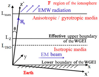
Figure 1 The geometry of the anisotropic and gyrotropic waveguide. EM waves propagate in the OX direction. H₀ is the external magnetic field. The effective WGEI for EM waves occupies the region $\mathrm{0}<z<L_z$. The isotropic medium occupies the region $\mathrm{0}<z<L_{\mathrm{ISO}}$, L_ISO<L_z. The anisotropic and gyrotropic medium occupies the region $L_{\mathrm{ISO}}<z<L_{\max }$. The covering layer occupies the region $L_z<z<L_{\max }$. WGEI includes the isotropic region $\mathrm{0}<z<L_{\mathrm{ISO}}$ and a part of the anisotropic region $L_z<z<L_{\max }$. It is supposed that the anisotropic region is relatively small part of the WG, $(L_z-L_{\mathrm{ISO}})/L_z\sim$ (0.1–0.2). At the upper boundary of the covering layer (z=L_max) EM radiation to the external region (z>L_max) is accounted for with the proper boundary conditions. The integration of the equations describing the EM field propagation allows for obtaining effective impedance boundary conditions at the upper boundary of the effective WG (z=L_z). These boundary conditions effectively include all the effects on the wave propagation of the covering layer and the radiation (at z=L_max) to the external region (z>L_max).

3 Algorithm

The boundary conditions and calculations of impedance and beam propagation in the WGEI are considered in this section. The other parts of the algorithm, e.g., the reflection of the EM waves from the WGEI effective upper boundary and the leakage of EM waves from the WGEI into the upper ionosphere and magnetosphere, will be presented very briefly as they are the subjects of the next papers.

3.1 Direct and inverse tensors characterizing the ionosphere

In the next subsections we derived the formulas describing the transfer of the boundary conditions at the upper boundary (z=L_max) (Fig. 1), resulting in the tensor impedance conditions at the upper boundary of the effective WGEI (z=L_i). Firstly let us describe the tensors characterizing the ionosphere.

The algorithm's main goal is to transfer the EM boundary conditions from the upper ionosphere at the height of L_z at ∼250–400 km to the lower ionosphere at L_z∼70–90 km. All components of the monochromatic EM field are considered to be proportional to exp (iωt). The anisotropic medium is inhomogeneous along OZ axis only and characterized by the permittivity tensor $\widehat{\mathit{\epsilon }}(\mathit{\omega },z)$ or by the inverse tensor $\widehat{\mathit{\beta }}(\mathit{\omega },z)={\widehat{\mathit{\epsilon }}}^{-\mathrm{1}}(\mathit{\omega },z)$: $\mathit{E}=\widehat{\mathit{\beta }}(\mathit{\omega },z)\cdot \mathit{D}$, where D is the electric induction. Below the absolute units are used. The expressions for the components of the effective permittivity of the ionosphere are in the coordinate frame $X^{\prime }Y{Z}^{\prime }$, where the OZ^′ axis is aligned along the geomagnetic field H₀.

$$\begin{array}{}\text{(1)}& \begin{array}{rl}{\widehat{\mathit{\epsilon }}}^{\prime }& =\left(\begin{array}{ccc}{\mathit{\epsilon }}_{\mathrm{1}}& {\mathit{\epsilon }}_h& \mathrm{0}\\ -{\mathit{\epsilon }}_h& {\mathit{\epsilon }}_{\mathrm{1}}& \mathrm{0}\\ \mathrm{0}& \mathrm{0}& {\mathit{\epsilon }}_{\mathrm{3}}\end{array}\right),\\ {\mathit{\epsilon }}_{\mathrm{1}}& =\mathrm{1}-{\displaystyle \frac{{\mathit{\omega }}_{\mathrm{pe}}^{\mathrm{2}}\cdot (\mathit{\omega }-i{\mathit{\nu }}_{\mathrm{e}})}{\left(\right(\mathit{\omega }-i{\mathit{\nu }}_{\mathrm{e}}{)}^{\mathrm{2}}-{\mathit{\omega }}_{H\mathrm{e}}^{\mathrm{2}})\cdot \mathit{\omega }}}\\ & -{\displaystyle \frac{{\mathit{\omega }}_{\mathrm{pi}}^{\mathrm{2}}\cdot (\mathit{\omega }-i{\mathit{\nu }}_{\mathrm{i}})}{\left(\right(\mathit{\omega }-i{\mathit{\nu }}_{\mathrm{i}}{)}^{\mathrm{2}}-{\mathit{\omega }}_{H\mathrm{i}}^{\mathrm{2}})\cdot \mathit{\omega }}},\\ {\mathit{\epsilon }}_h& \equiv ig;\\ g& =-{\displaystyle \frac{{\mathit{\omega }}_{\mathrm{pe}}^{\mathrm{2}}\cdot {\mathit{\omega }}_{H\mathrm{e}}}{\left(\right(\mathit{\omega }-i{\mathit{\nu }}_{\mathrm{e}}{)}^{\mathrm{2}}-{\mathit{\omega }}_{H\mathrm{e}}^{\mathrm{2}})\cdot \mathit{\omega }}}\\ & +{\displaystyle \frac{{\mathit{\omega }}_{\mathrm{pi}}^{\mathrm{2}}\cdot {\mathit{\omega }}_{H\mathrm{i}}}{\left(\right(\mathit{\omega }-i{\mathit{\nu }}_{\mathrm{i}}{)}^{\mathrm{2}}-{\mathit{\omega }}_{H\mathrm{i}}^{\mathrm{2}})\cdot \mathit{\omega }}},\\ {\mathit{\epsilon }}_{\mathrm{3}}& =\mathrm{1}-{\displaystyle \frac{{\mathit{\omega }}_{\mathrm{pe}}^{\mathrm{2}}}{(\mathit{\omega }-i{\mathit{\nu }}_{\mathrm{e}})\cdot \mathit{\omega }}}-{\displaystyle \frac{{\mathit{\omega }}_{\mathrm{pi}}^{\mathrm{2}}}{(\mathit{\omega }-i{\mathit{\nu }}_{\mathrm{i}})\cdot \mathit{\omega }}};\\ {\mathit{\omega }}_{\mathrm{pe}}^{\mathrm{2}}& ={\displaystyle \frac{\mathrm{4}\mathit{\pi }{e}^{\mathrm{2}}n}{m_{\mathrm{e}}}},\\ {\mathit{\omega }}_{\mathrm{pi}}^{\mathrm{2}}& ={\displaystyle \frac{\mathrm{4}\mathit{\pi }{e}^{\mathrm{2}}n}{m_{\mathrm{i}}}},\\ {\mathit{\omega }}_{H\mathrm{e}}& ={\displaystyle \frac{e{H}_{\mathrm{0}}}{m_{\mathrm{e}}c}},\\ {\mathit{\omega }}_{H\mathrm{i}}& ={\displaystyle \frac{e{H}_{\mathrm{0}}}{m_{\mathrm{i}}c}},\end{array}\end{array}$$

where ω_pe, ω_pi, ω_He and ω_Hi are the plasma and cyclotron frequencies for electrons and ions, respectively, m_e, m_i, ν_e and ν_i are the masses and collision frequencies for electrons and ions, respectively, and n is the electron concentration. The approximations of the three-component plasma-like ionosphere (including one electron component, one effective ion and one effective neutral component) and quasi-neutrality are accepted. The expressions for the components of the permittivity tensor $\widehat{\mathit{\epsilon }}(\mathit{\omega }$, z) are obtained from Eq. (1) by means of multiplication with the standard rotation matrices (Spiegel, 1959) dependent on angle θ. For the medium with a scalar conductivity σ, e.g., lower ionosphere or atmosphere, the effective permittivity in Eq. (1) reduces to $\mathit{\epsilon }=\mathrm{1}-\mathrm{4}\mathit{\pi }i\mathit{\sigma }/\mathit{\omega }$.

3.2 The equations for the EM field and upper boundary conditions

In the case of the VLF waveguide modes, the longitudinal wave number k_x is slightly complex and should be calculated accounting for boundary conditions at the Earth's surface and the upper surface of the effective WGEI. The EM field depends on the horizontal coordinate x as exp (−ik_xx). Taking into account k_x≈k₀ $(k_{\mathrm{0}}=\mathit{\omega }/c)$, in simulations of the VLF beam propagation, it is possible to put k_x=k₀. Therefore, Maxwell's equations are

$$\begin{array}{}\text{(2)}& \begin{array}{rl}& -{\displaystyle \frac{\partial H_y}{\partial z}}=i{k}_{\mathrm{0}}{D}_x,{\displaystyle \frac{\partial H_x}{\partial z}}+i{k}_x{H}_z=i{k}_{\mathrm{0}}{D}_y,\\ & -i{k}_x{H}_y=i{k}_{\mathrm{0}}{D}_z\\ & -{\displaystyle \frac{\partial E_y}{\partial z}}=-i{k}_{\mathrm{0}}{H}_x,{\displaystyle \frac{\partial E_x}{\partial z}}+i{k}_x{E}_z=-i{k}_{\mathrm{0}}{H}_y,\\ & -i{k}_x{E}_y=-i{k}_{\mathrm{0}}{H}_z,\end{array}\end{array}$$

where $E_x={\mathit{\beta }}_{\mathrm{11}}{D}_x+{\mathit{\beta }}_{\mathrm{12}}{D}_y+{\mathit{\beta }}_{\mathrm{13}}{D}_z$, etc. All components of the EM field can be represented through the horizontal components of the magnetic field H_x and H_y. The equations for these components are given below.

$$\begin{array}{}\text{(3a)}& {\displaystyle }\begin{array}{rl}& {\displaystyle \frac{\partial }{\partial z}}\left({\displaystyle \frac{{\mathit{\beta }}_{\mathrm{22}}}{\mathrm{1}-{\mathit{\beta }}_{\mathrm{22}}\frac{k_x^{\mathrm{2}}}{k_{\mathrm{0}}^{\mathrm{2}}}}}{\displaystyle \frac{\partial H_x}{\partial z}}\right)-{\displaystyle \frac{\partial }{\partial z}}\left({\displaystyle \frac{{\mathit{\beta }}_{\mathrm{21}}}{\mathrm{1}-{\mathit{\beta }}_{\mathrm{22}}\frac{k_x^{\mathrm{2}}}{k_{\mathrm{0}}^{\mathrm{2}}}}}{\displaystyle \frac{\partial H_y}{\partial z}}\right)\\ & -i{k}_x{\displaystyle \frac{\partial }{\partial z}}\left({\displaystyle \frac{{\mathit{\beta }}_{\mathrm{23}}}{\mathrm{1}-{\mathit{\beta }}_{\mathrm{22}}\frac{k_x^{\mathrm{2}}}{k_{\mathrm{0}}^{\mathrm{2}}}}}{H}_y\right)+k_{\mathrm{0}}^{\mathrm{2}}{H}_x=\mathrm{0}\end{array}\text{(3b)}& {\displaystyle }\begin{array}{rl}& {\displaystyle \frac{\partial }{\partial z}}\left(\left({\mathit{\beta }}_{\mathrm{11}}+{\displaystyle \frac{k_x^{\mathrm{2}}}{k_{\mathrm{0}}^{\mathrm{2}}}}{\displaystyle \frac{{\mathit{\beta }}_{\mathrm{12}}\cdot {\mathit{\beta }}_{\mathrm{21}}}{\mathrm{1}-{\mathit{\beta }}_{\mathrm{22}}\frac{k_x^{\mathrm{2}}}{k_{\mathrm{0}}^{\mathrm{2}}}}}\right){\displaystyle \frac{\partial H_y}{\partial z}}\right)-{\displaystyle \frac{\partial }{\partial z}}\left({\displaystyle \frac{{\mathit{\beta }}_{\mathrm{12}}}{\mathrm{1}-{\mathit{\beta }}_{\mathrm{22}}\frac{k_x^{\mathrm{2}}}{k_{\mathrm{0}}^{\mathrm{2}}}}}{\displaystyle \frac{\partial H_x}{\partial z}}\right)\\ & +i{k}_x{\displaystyle \frac{\partial }{\partial z}}\left(\left({\mathit{\beta }}_{\mathrm{13}}+{\displaystyle \frac{k_x^{\mathrm{2}}}{k_{\mathrm{0}}^{\mathrm{2}}}}{\displaystyle \frac{{\mathit{\beta }}_{\mathrm{12}}\cdot {\mathit{\beta }}_{\mathrm{23}}}{\mathrm{1}-{\mathit{\beta }}_{\mathrm{22}}\frac{k_x^{\mathrm{2}}}{k_{\mathrm{0}}^{\mathrm{2}}}}}\right)H_y\right)\\ & +i{k}_x\left({\mathit{\beta }}_{\mathrm{31}}+{\displaystyle \frac{k_x^{\mathrm{2}}}{k_{\mathrm{0}}^{\mathrm{2}}}}{\displaystyle \frac{{\mathit{\beta }}_{\mathrm{32}}\cdot {\mathit{\beta }}_{\mathrm{21}}}{\mathrm{1}-{\mathit{\beta }}_{\mathrm{22}}\frac{k_x^{\mathrm{2}}}{k_{\mathrm{0}}^{\mathrm{2}}}}}\right){\displaystyle \frac{\partial H_y}{\partial z}}-\\ & -i{k}_x{\displaystyle \frac{{\mathit{\beta }}_{\mathrm{32}}}{\mathrm{1}-{\mathit{\beta }}_{\mathrm{22}}\frac{k_x^{\mathrm{2}}}{k_{\mathrm{0}}^{\mathrm{2}}}}}{\displaystyle \frac{\partial H_x}{\partial z}}\\ & +k_{\mathrm{0}}^{\mathrm{2}}\left(\mathrm{1}-{\mathit{\beta }}_{\mathrm{33}}{\displaystyle \frac{k_x^{\mathrm{2}}}{k_{\mathrm{0}}^{\mathrm{2}}}}-{\displaystyle \frac{k_x^{\mathrm{4}}}{k_{\mathrm{0}}^{\mathrm{4}}}}{\displaystyle \frac{{\mathit{\beta }}_{\mathrm{23}}\cdot {\mathit{\beta }}_{\mathrm{32}}}{\mathrm{1}-{\mathit{\beta }}_{\mathrm{22}}\frac{k_x^{\mathrm{2}}}{k_{\mathrm{0}}^{\mathrm{2}}}}}\right)H_y=\mathrm{0}\end{array}\end{array}$$

The expressions for the horizontal components of the electric field E_x, E_y are given below.

$$\begin{array}{}\text{(4)}& \begin{array}{rl}{E}_x& ={\displaystyle \frac{i}{k_{\mathrm{0}}}}\left(\left({\mathit{\beta }}_{\mathrm{11}}+{\displaystyle \frac{k_x^{\mathrm{2}}}{k_{\mathrm{0}}^{\mathrm{2}}}}{\displaystyle \frac{{\mathit{\beta }}_{\mathrm{12}}\cdot {\mathit{\beta }}_{\mathrm{21}}}{\mathrm{1}-{\mathit{\beta }}_{\mathrm{22}}\frac{k_x^{\mathrm{2}}}{k_{\mathrm{0}}^{\mathrm{2}}}}}\right){\displaystyle \frac{\partial H_y}{\partial z}}-{\displaystyle \frac{{\mathit{\beta }}_{\mathrm{12}}}{\mathrm{1}-{\mathit{\beta }}_{\mathrm{22}}\frac{k_x^{\mathrm{2}}}{k_{\mathrm{0}}^{\mathrm{2}}}}}{\displaystyle \frac{\partial H_y}{\partial z}}\right)\\ & -{\displaystyle \frac{k_x}{k_{\mathrm{0}}}}\left({\mathit{\beta }}_{\mathrm{13}}+{\displaystyle \frac{k_x^{\mathrm{2}}}{k_{\mathrm{0}}^{\mathrm{2}}}}{\displaystyle \frac{{\mathit{\beta }}_{\mathrm{12}}\cdot {\mathit{\beta }}_{\mathrm{23}}}{\mathrm{1}-{\mathit{\beta }}_{\mathrm{22}}\frac{k_x^{\mathrm{2}}}{k_{\mathrm{0}}^{\mathrm{2}}}}}\right)H_y\\ E_y& ={\displaystyle \frac{i}{k_{\mathrm{0}}}}\left(-{\displaystyle \frac{{\mathit{\beta }}_{\mathrm{22}}}{\mathrm{1}-{\mathit{\beta }}_{\mathrm{22}}\frac{k_x^{\mathrm{2}}}{k_{\mathrm{0}}^{\mathrm{2}}}}}{\displaystyle \frac{\partial H_x}{\partial z}}+{\displaystyle \frac{{\mathit{\beta }}_{\mathrm{21}}}{\mathrm{1}-{\mathit{\beta }}_{\mathrm{22}}\frac{k_x^{\mathrm{2}}}{k_{\mathrm{0}}^{\mathrm{2}}}}}{\displaystyle \frac{\partial H_y}{\partial z}}\right)\\ & -{\displaystyle \frac{k_x}{k_{\mathrm{0}}}}{\displaystyle \frac{{\mathit{\beta }}_{\mathrm{23}}}{\mathrm{1}-{\mathit{\beta }}_{\mathrm{22}}\frac{k_x^{\mathrm{2}}}{k_{\mathrm{0}}^{\mathrm{2}}}}}{H}_y\end{array}\end{array}$$

In the region z≥L_max the upper ionosphere is assumed to be weakly inhomogeneous, and the geometric optics approximation is valid in the VLF range there. We should note that due to high inhomogeneity of the ionosphere in the vertical direction within the E layer (i.e., at the upper boundary of the effective VLF WGEI) such an approximation is not applicable. These conditions determine the choice of the upper boundary of z=L_max at ∼ 250–400 km, where the conditions of the radiation are formulated. The dispersion equation which connected the wave numbers and the frequency of the outgoing waves is obtained from Eq. (3a, 3b), where $H_{x,y}\sim \exp (-i{k}_{z}z)$, while the derivatives like $\partial {\mathit{\beta }}_{\mathrm{11}}/\partial z$ and the inhomogeneity of the media are neglected.

$$\begin{array}{}\text{(5)}& \begin{array}{rl}& \left({\mathit{\beta }}_{\mathrm{22}}{k}_z^{\mathrm{2}}-k_{\mathrm{0}}^{\mathrm{2}}\left(\mathrm{1}-{\mathit{\beta }}_{\mathrm{22}}{\displaystyle \frac{k_x^{\mathrm{2}}}{k_{\mathrm{0}}^{\mathrm{2}}}}\right)\right)\cdot \left(\left({\mathit{\beta }}_{\mathrm{11}}\left(\mathrm{1}-{\mathit{\beta }}_{\mathrm{22}}{\displaystyle \frac{k_x^{\mathrm{2}}}{k_{\mathrm{0}}^{\mathrm{2}}}}\right)\right.\right.\\ & \left.+{\displaystyle \frac{k_x^{\mathrm{2}}}{k_{\mathrm{0}}^{\mathrm{2}}}}{\mathit{\beta }}_{\mathrm{12}}\cdot {\mathit{\beta }}_{\mathrm{21}}\right)k_z^{\mathrm{2}}\\ & +({\mathit{\beta }}_{\mathrm{13}}+{\mathit{\beta }}_{\mathrm{31}})\left(\mathrm{1}-{\mathit{\beta }}_{\mathrm{22}}{\displaystyle \frac{k_x^{\mathrm{2}}}{k_{\mathrm{0}}^{\mathrm{2}}}}\right)+\\ & {\displaystyle \frac{k_x^{\mathrm{2}}}{k_{\mathrm{0}}^{\mathrm{2}}}}({\mathit{\beta }}_{\mathrm{12}}\cdot {\mathit{\beta }}_{\mathrm{23}}+{\mathit{\beta }}_{\mathrm{32}}\cdot {\mathit{\beta }}_{\mathrm{21}})k_x{k}_z\\ & \left.-k_{\mathrm{0}}^{\mathrm{2}}\left(\left(\mathrm{1}-{\mathit{\beta }}_{\mathrm{33}}{\displaystyle \frac{k_x^{\mathrm{2}}}{k_{\mathrm{0}}^{\mathrm{2}}}}\right)\left(\mathrm{1}-{\mathit{\beta }}_{\mathrm{22}}{\displaystyle \frac{k_x^{\mathrm{2}}}{k_{\mathrm{0}}^{\mathrm{2}}}}\right)-{\displaystyle \frac{k_x^{\mathrm{4}}}{k_{\mathrm{0}}^{\mathrm{4}}}}{\mathit{\beta }}_{\mathrm{23}}\cdot {\mathit{\beta }}_{\mathrm{32}}\right)\right)-\\ & -({\mathit{\beta }}_{\mathrm{21}}{k}_z^{\mathrm{2}}+{\mathit{\beta }}_{\mathrm{23}}{k}_x{k}_z)\cdot ({\mathit{\beta }}_{\mathrm{12}}{k}_z^{\mathrm{2}}-{\mathit{\beta }}_{\mathrm{32}}{k}_x{k}_z)=\mathrm{0}\end{array}\end{array}$$

Thus, generally Eq. (5) determined the wave numbers for the outgoing waves to be of the fourth order (Wait, 1996). The boundary conditions at the upper boundary z=L_max within the ionosphere F layer are the absence of the ingoing waves, i.e., the outgoing radiated (leakage) waves are present only. Two roots should be selected that possess the negative imaginary parts $\mathrm{Im}\left(k_{z\mathrm{1},z\mathrm{2}}\right)<\mathrm{0}$; i.e., the outgoing waves dissipate upwards. However, in the case of VLF waves, some simplification can be used. Namely, the expressions for the wave numbers k_1,2 are obtained from Eq. (3a, 3b), where the dependence on x is neglected: $\left|k_{\mathrm{1},\mathrm{2}}\right|\gg k_{\mathrm{0}}$. This approximation is valid within the F layer where the first outgoing wave corresponds to the whistlers with a small dissipation; the second one is the highly dissipating slow wave. To formulate the boundary conditions for Eq. (3a, 3b) at z≥L_max, the EM field components can be presented as

$$\begin{array}{}\text{(6)}& \begin{array}{rl}{H}_x& =A_{\mathrm{1}}{e}^{-i{k}_{z\mathrm{1}}\stackrel{\mathrm{̃}}{z}}+{\mathit{\alpha }}_{\mathrm{2}}{A}_{\mathrm{2}}{e}^{-i{k}_{z\mathrm{2}}\stackrel{\mathrm{̃}}{z}},\\ H_y& ={\mathit{\alpha }}_{\mathrm{1}}{A}_{\mathrm{1}}{e}^{-i{k}_{z\mathrm{1}}\stackrel{\mathrm{̃}}{z}}+A_{\mathrm{2}}{e}^{-i{k}_{z\mathrm{2}}\stackrel{\mathrm{̃}}{z}}.\end{array}\end{array}$$

In Eq. (6), $\stackrel{\mathrm{̃}}{z}=z-L_z$ . Equation (3a, 3b) are simplified in the approximation described above.

$$\begin{array}{}\text{(7)}& \begin{array}{rl}{\mathit{\beta }}_{\mathrm{22}}{\displaystyle \frac{{\partial }^{\mathrm{2}}{H}_x}{\partial z^{\mathrm{2}}}}& -{\mathit{\beta }}_{\mathrm{21}}{\displaystyle \frac{{\partial }^{\mathrm{2}}{H}_y}{\partial z^{\mathrm{2}}}}+k_{\mathrm{0}}^{\mathrm{2}}{H}_x=\mathrm{0},\\ {\mathit{\beta }}_{\mathrm{11}}{\displaystyle \frac{{\partial }^{\mathrm{2}}{H}_y}{\partial z^{\mathrm{2}}}}& -{\mathit{\beta }}_{\mathrm{12}}{\displaystyle \frac{{\partial }^{\mathrm{2}}{H}_x}{\partial z^{\mathrm{2}}}}+k_{\mathrm{0}}^{\mathrm{2}}{H}_y=\mathrm{0}\end{array}\end{array}$$

The solution of Eq. (7) is searched for as $H_{x,y}\sim \exp (-i{k}_z\stackrel{\mathrm{̃}}{z})$. The following equation has been obtained to get the wave numbers k_z1,z2 from Eq. (7):

$$\begin{array}{}\text{(8)}& \begin{array}{rl}& {\mathit{\kappa }}^{\mathrm{4}}-({\mathit{\beta }}_{\mathrm{22}}+{\mathit{\beta }}_{\mathrm{11}}){\mathit{\kappa }}^{\mathrm{2}}+{\mathit{\beta }}_{\mathrm{11}}{\mathit{\beta }}_{\mathrm{22}}-{\mathit{\beta }}_{\mathrm{12}}{\mathit{\beta }}_{\mathrm{21}}=\mathrm{0},\\ & {\mathit{\kappa }}^{\mathrm{2}}={\displaystyle \frac{k_{\mathrm{0}}^{\mathrm{2}}}{k_z^{\mathrm{2}}}}.\end{array}\end{array}$$

Therefore, from Eq. (8) follows,

$$\begin{array}{}\text{(9)}& {\displaystyle }\begin{array}{rl}{\mathit{\kappa }}_{\mathrm{1},\mathrm{2}}^{\mathrm{2}}& ={\displaystyle \frac{{\mathit{\beta }}_{\mathrm{11}}+{\mathit{\beta }}_{\mathrm{22}}}{\mathrm{2}}}\pm {\left({\left({\displaystyle \frac{{\mathit{\beta }}_{\mathrm{11}}+{\mathit{\beta }}_{\mathrm{22}}}{\mathrm{2}}}\right)}^{\mathrm{2}}+{\mathit{\beta }}_{\mathrm{12}}{\mathit{\beta }}_{\mathrm{21}}\right)}^{\mathrm{1}/\mathrm{2}};\\ {\mathit{\alpha }}_{\mathrm{1}}& ={\displaystyle \frac{{\mathit{\beta }}_{\mathrm{22}}-{\mathit{\kappa }}_{\mathrm{1}}^{\mathrm{2}}}{{\mathit{\beta }}_{\mathrm{21}}}}={\displaystyle \frac{{\mathit{\beta }}_{\mathrm{12}}}{{\mathit{\beta }}_{\mathrm{11}}-{\mathit{\kappa }}_{\mathrm{1}}^{\mathrm{2}}}};\\ {\mathit{\alpha }}_{\mathrm{2}}& ={\displaystyle \frac{{\mathit{\beta }}_{\mathrm{11}}-{\mathit{\kappa }}_{\mathrm{2}}^{\mathrm{2}}}{{\mathit{\beta }}_{\mathrm{12}}}}={\displaystyle \frac{{\mathit{\beta }}_{\mathrm{21}}}{{\mathit{\beta }}_{\mathrm{22}}-{\mathit{\kappa }}_{\mathrm{2}}^{\mathrm{2}}}};\\ k_{z\mathrm{1},z\mathrm{2}}^{\mathrm{2}}& ={\displaystyle \frac{k_{\mathrm{0}}^{\mathrm{2}}}{{\mathit{\kappa }}_{\mathrm{1},\mathrm{2}}^{\mathrm{2}}}}.\end{array}\end{array}$$

The signs of k_z1,z2 have been chosen from the condition $\mathrm{Im}\left(k_{z\mathrm{1},z\mathrm{2}}\right)<\mathrm{0}$. From Eq. (5) at the upper boundary of z=L_max, the following relations are valid:

$$\begin{array}{}\text{(10)}& H_x=A_{\mathrm{1}}+{\mathit{\alpha }}_{\mathrm{2}}{A}_{\mathrm{2}},H_y={\mathit{\alpha }}_{\mathrm{1}}{A}_{\mathrm{1}}+A_{\mathrm{2}}.\end{array}$$

From Eq. (10) one can get

$$\begin{array}{}\text{(11)}& \begin{array}{rl}{A}_{\mathrm{1}}& ={\mathrm{\Delta }}^{-\mathrm{1}}(H_x-{\mathit{\alpha }}_{\mathrm{2}}{H}_y);A_{\mathrm{2}}={\mathrm{\Delta }}^{-\mathrm{1}}(H_y-{\mathit{\alpha }}_{\mathrm{1}}{H}_x);\\ \mathrm{\Delta }& =\mathrm{1}-{\mathit{\alpha }}_{\mathrm{1}}{\mathit{\alpha }}_{\mathrm{2}}.\end{array}\end{array}$$

Thus, it is possible to exclude the amplitudes of the outgoing waves A_1,2 from Eqs. (9). As a result, at z=L_max the boundary conditions are rewritten in terms of H_x and H_y only.

$$\begin{array}{}\text{(12)}& \begin{array}{rl}{\displaystyle \frac{\partial H_x}{\partial z}}& =-i(k_{z\mathrm{1}}{A}_{\mathrm{1}}+k_{z\mathrm{2}}{\mathit{\alpha }}_{\mathrm{2}}{A}_{\mathrm{2}})\\ & =-{\displaystyle \frac{i}{\mathrm{\Delta }}}\left(\right(k_{z\mathrm{1}}-{\mathit{\alpha }}_{\mathrm{1}}{\mathit{\alpha }}_{\mathrm{2}}{k}_{z\mathrm{2}})H_x+{\mathit{\alpha }}_{\mathrm{2}}(k_{z\mathrm{2}}-k_{z\mathrm{1}}\left)H_y\right)\\ {\displaystyle \frac{\partial H_y}{\partial z}}& =-i(k_{z\mathrm{1}}{\mathit{\alpha }}_{\mathrm{1}}{A}_{\mathrm{1}}+k_{z\mathrm{2}}{A}_{\mathrm{2}})\\ & =-{\displaystyle \frac{i}{\mathrm{\Delta }}}\left(\right(k_{z\mathrm{2}}-{\mathit{\alpha }}_{\mathrm{1}}{\mathit{\alpha }}_{\mathrm{2}}{k}_{z\mathrm{1}})H_y+{\mathit{\alpha }}_{\mathrm{1}}(k_{z\mathrm{1}}-k_{z\mathrm{2}}\left)H_x\right)\end{array}\end{array}$$

The relations in Eq. (12) are the upper boundary conditions of the radiation for the boundary z=L_max at ∼250–400 km. These conditions will be transformed and recalculated using the analytical numerical recurrent procedure into equivalent impedance boundary conditions at z=L_z at ∼70–90 km.

Note that in the “whistler–VLF approximation” is valid at frequencies ∼10 kHz for the F region of the ionosphere. In this approximation and k_x≈0, we receive the dispersion equation using Eqs. (5), (8), (9), in the form

$$\begin{array}{}\text{(13)}& {k_z^{\prime }}^{\mathrm{2}}{k}^{\mathrm{2}}=k_{\mathrm{0}}^{\mathrm{2}}{g}^{\mathrm{2}},\end{array}$$

where $k^{\mathrm{2}}=k_x^{\mathrm{2}}+k_z^{\mathrm{2}}={k_x^{\prime }}^{\mathrm{2}}+{k_z^{\prime }}^{\mathrm{2}}$ and $k_x^{\prime }$ and $k_z^{\prime }$ are the transverse and longitudinal components of the wave number relative to geomagnetic field. For the F region of the ionosphere, where ${\mathit{\nu }}_{\mathrm{e}}\ll \mathit{\omega }\ll {\mathit{\omega }}_{H\mathrm{e}}$, Eq. (13) reduces to the standard form of the whistler dispersion equation $\left|k_z^{\prime }\right|k=k_{\mathrm{0}}\left|g\right|$, $g\approx -{\mathit{\omega }}_{\mathrm{pe}}^{\mathrm{2}}/\left(\mathit{\omega }{\mathit{\omega }}_{H\mathrm{e}}\right)$ and $\mathit{\omega }=c^{\mathrm{2}}k\left|k_z^{\prime }\right|({\mathit{\omega }}_{H\mathrm{e}}/{\mathit{\omega }}_{\mathrm{pe}}^{\mathrm{2}})$. In a special case of the waves propagating along geomagnetic field, $k_x^{\prime }=\mathrm{0}$, for the propagating whistler waves, the well-known dispersion dependence is $\mathit{\omega }=c^{\mathrm{2}}{k_z^{\prime }}^{\mathrm{2}}({\mathit{\omega }}_{H\mathrm{e}}/{\mathit{\omega }}_{\mathrm{pe}}^{\mathrm{2}})$ (Artsimovich and Sagdeev, 1979). For the formulated problem we can reasonably assume k_x≈0. Therefore Eq. (13) is reduced to $k_z^{\mathrm{4}}{\cos }^{\mathrm{2}}\mathit{\theta }=k_{\mathrm{0}}^{\mathrm{4}}{g}^{\mathrm{2}}$. As a result, we get $k_{z\mathrm{1}}=\sqrt{g/\cos \mathit{\theta }}{k}_{\mathrm{0}}$ and $k_{z\mathrm{2}}=-i\sqrt{g/\cos \mathit{\theta }}{k}_{\mathrm{0}}$, and then, similar to the relations in Eq. (12), the boundary conditions can be presented in terms of the tangential components of the electric field as

$$\begin{array}{}\text{(14)}& \begin{array}{rl}& {\displaystyle \frac{\partial \mathit{U}}{\partial z}}+\widehat{B}\mathit{U}=\mathrm{0};\\ & \mathit{U}=\left(\begin{array}{c}{E}_x\\ E_y\end{array}\right);\\ & \widehat{B}={\displaystyle \frac{\mathrm{1}}{\mathrm{2}}}\sqrt{{\displaystyle \frac{g}{\cos \mathit{\theta }}}}{k}_{\mathrm{0}}\left(\begin{array}{cc}\mathrm{1}+i& -\mathrm{1}-i\\ \mathrm{1}+i& \mathrm{1}+i\end{array}\right).\end{array}\end{array}$$

Conditions in Eq. (12) or Eq. (14) are the conditions of radiation (absence of ingoing waves) formulated at the upper boundary at z=L_max and suitable for the determination of the energy of the wave leaking from the WGEI into the upper ionosphere and magnetosphere. Note that Eqs. (12) and (14) expressed the boundary conditions of the radiation (more accurately speaking, an absence of incoming waves, which is the consequence to the causality principle) are obtained as a result of the passage to limit $|k_x/k_z|\to \mathrm{0}$ in Eq. (5). In spite of the disappearance of the dependence of these boundary conditions explicitly on k_x, the dependence of the characteristics of the wave propagation process on k_x, as a whole, is accounted for, and all results are still valid for the description of the wave beam propagation in the WGEI along the horizontal axis x with a finite k_x∼k₀.

3.3 Equivalent tensor impedance boundary conditions

The tensor impedance at the upper boundary of the effective WGEI of z=L_z (see Fig. 1) is obtained by the conditions of radiation in Eqs. (12) or (14), recalculated from the level of $z=L_{\max }\sim \mathrm{250}$–400 km, placed in the F region of the ionosphere, to the level of $z=L_z\sim \mathrm{80}$–90 km, placed in the E region.

The main idea of the effective tensor impedance method is the unification of analytical and numerical approaches and the derivation of the proper impedance boundary conditions without “thin-cover-layer” approximation. This approximation is usually used in the effective impedance approaches, applied either for artificial or natural layered gyrotropic structures (see e.g., Tretyakov, 2003; Senior and Volakis, 1995; Kurushin and Nefedov, 1983; Alperovich and Fedorov, 2007). There is one known exception, namely the invariant imbedding impedance method (Shalashov and Gospodchikov, 2011; Kim and Kim, 2016). The comparison of our method with the invariant imbedding impedance method will be presented at the end of this subsection. Equation (3a, 3b) jointly with the boundary conditions of Eq. (12) have been solved by finite differences. The derivatives in Eq. (3a, 3b) are approximated as

$$\begin{array}{}\text{(15)}& \begin{array}{rl}{\displaystyle \frac{\partial }{\partial z}}\left(C\left(z\right){\displaystyle \frac{\partial H_x}{\partial z}}\right)& \approx {\displaystyle \frac{\mathrm{1}}{h}}\left(C\left(z_{j+\mathrm{1}/\mathrm{2}}\right){\displaystyle \frac{(H_x{)}_{j+\mathrm{1}}-(H_x{)}_j}{h}}\right.\\ & \left.-C\left(z_{j-\mathrm{1}/\mathrm{2}}\right){\displaystyle \frac{(H_x{)}_j-(H_x{)}_{j-\mathrm{1}}}{h}}\right)\\ {\displaystyle \frac{\partial }{\partial z}}\left(F\right(z\left)H_x\right)& \approx {\displaystyle \frac{\mathrm{1}}{\mathrm{2}h}}\left(F\right(z_{j+\mathrm{1}}\left)\right(H_x{)}_{j+\mathrm{1}}\\ & -F\left(z_{j-\mathrm{1}}\right)\left(H_x{)}_{j-\mathrm{1}}\right).\end{array}\end{array}$$

In Eq. (15) $z_{j+\mathrm{1}/\mathrm{2}}=h\cdot (j+\mathrm{0.5})$. In Eq. (10) the approximation is $\partial H_x/\partial z\approx \left[\right(H_x{)}_N-\left(H_x{)}_{N-\mathrm{1}}\right]/h$. Here h is the discretization step along the OZ axis, and N is the total number of nodes. At each step j the difference approximations of Eq. (3a, 3b) take the form

$$\begin{array}{}\text{(16)}& {\widehat{\mathit{\alpha }}}_j^{(-)}\cdot {\mathit{H}}_{j-\mathrm{1}}+{\widehat{\mathit{\alpha }}}_j^{\left(\mathrm{0}\right)}\cdot {\mathit{H}}_j+{\widehat{\mathit{\alpha }}}_j^{(+)}\cdot {\mathit{H}}_{j+\mathrm{1}}=\mathrm{0},\end{array}$$

where ${\mathit{H}}_j=\left(\begin{array}{c}{H}_x\\ h_y\end{array}\right)$, $j=N-\mathrm{1},N-\mathrm{2},\mathrm{\dots },\mathrm{1}$, $z_j=h\cdot j$ and $L_z=h\cdot N$. Due to the complexity of expressions for the matrix coefficients in Eq. (16), we have shown them in Appendix A. The set of the matrix Eq. (16) has been solved by the factorization method also known as an elimination and matrix sweep method (see Samarskii, 2001). It can be written as

$$\begin{array}{}\text{(17a)}& {\displaystyle }{\mathit{H}}_j={\widehat{b}}_j\cdot {\mathit{H}}_{j+\mathrm{1}},j=N,\mathrm{\dots }\mathrm{1}\text{(17b)}& {\displaystyle }\begin{array}{rl}& H_{xj+\mathrm{1}}=b_{\mathrm{11}j+\mathrm{1}}{H}_{\mathrm{1}}+b_{\mathrm{12}j+\mathrm{1}}{H}_{\mathrm{2}};\\ & H_{yj+\mathrm{1}}=b_{\mathrm{21}j+\mathrm{1}}{H}_{\mathrm{1}}+b_{\mathrm{22}j+\mathrm{1}}{H}_{\mathrm{2}};\\ & H_{\mathrm{1}}\equiv H_{xj};\\ & H_{\mathrm{2}}\equiv H_{yj}\end{array}.\end{array}$$

This method is a variant of the Gauss elimination method for the matrix three-diagonal set of Eq. (16). The value of ${\widehat{b}}_N$ is obtained from the boundary conditions (12) as

$$\begin{array}{}\text{(18)}& {\widehat{\mathit{\alpha }}}_N^{(-)}\cdot {\mathit{H}}_{N-\mathrm{1}}+{\widehat{\mathit{\alpha }}}_N^{\left(\mathrm{0}\right)}\cdot {\mathit{H}}_N=\mathrm{0}.\end{array}$$

Therefore ${\widehat{b}}_N=-({\widehat{\mathit{\alpha }}}_N^{\left(\mathrm{0}\right)}{)}^{-\mathrm{1}}\cdot {\widehat{\mathit{\alpha }}}_N^{(-)}$. Then the matrices ${\widehat{b}}_j$ have been computed sequentially down to the desired value of $z=L_z=h\cdot N_z$, where the impedance boundary conditions are assumed to be applied. At each step the expression for ${\widehat{b}}_j$ follows from Eqs. (16), (17a) and (17b) as

$$\begin{array}{}\text{(19)}& ({\widehat{\mathit{\alpha }}}_j^{\left(\mathrm{0}\right)}+{\widehat{\mathit{\alpha }}}_j^{(+)}\cdot {\widehat{b}}_{j+\mathrm{1}})\cdot {\mathit{H}}_j=-{\widehat{\mathit{\alpha }}}_j^{(-)}\cdot {\mathit{H}}_{j-\mathrm{1}}=\mathrm{0}.\end{array}$$

Therefore, for Eq. (17a, 17b), we obtain ${\widehat{b}}_j=-({\widehat{\mathit{\alpha }}}_j^{\left(\mathrm{0}\right)}+{\widehat{\mathit{\alpha }}}_j^{(+)}\cdot {\widehat{b}}_{j+\mathrm{1}}{)}^{-\mathrm{1}}\cdot {\widehat{\mathit{\alpha }}}_j^{(-)}$. The derivatives in Eq. (4) have been approximated as

$$\begin{array}{}\text{(20)}& \begin{array}{rl}{\left({\displaystyle \frac{\partial H_x}{\partial z}}\right)}_{N_z}& \approx {\displaystyle \frac{(H_x{)}_{N_z+\mathrm{1}}-(H_x{)}_{N_z}}{h}}\\ & ={\displaystyle \frac{(b_{N_z+\mathrm{1}\mathrm{11}}-\mathrm{1})\cdot (H_x{)}_{N_z}+b_{N_z+\mathrm{1}\mathrm{12}}\cdot (H_y{)}_{N_z}}{h}},\end{array}\end{array}$$

and a similar equation can be obtained for ${\left(\frac{\partial H_y}{\partial z}\right)}_{N_z}$. Note that as a result of this discretization, only the values at the grid level N_z are included in the numerical approximation of the derivatives $\partial H_{x,y}/\partial z$ at z=L_z. We determine tensor impedance $\widehat{Z}$ at z=L_z at ∼85 km. The tensor values are included in the following relations, all of which are corresponded to altitude (in other words, to the grid with the number N_z and corresponding to this altitude).

$$\begin{array}{}\text{(21)}& \begin{array}{rl}& \mathit{n}\times \mathit{E}=\widehat{Z_{\mathrm{0}}}\cdot \mathit{H},\mathit{n}=(\mathrm{0},\mathrm{0},\mathrm{1})\text{ or }\\ & E_x=Z_{\mathrm{021}}{H}_x+Z_{\mathrm{022}}{H}_y;E_y=-Z_{\mathrm{011}}{H}_x-Z_{\mathrm{012}}{H}_y\end{array}\end{array}$$

The equivalent tensor impedance is obtained using a two-step procedure. (1) We obtain the matrix ${\widehat{b}}_j$ using Eq. (3a, 3b) with the boundary conditions of Eq. (12) and the procedure of Eqs. (17)–(19) described above. (2) Placing the expressions of Eq. (21) with tensor impedance into the left parts and the derivatives $\partial H_{x,y}/\partial z$ in Eq. (20) into the right parts of Eq. (4), the analytical expressions for the components of the tensor impedance are

$$\begin{array}{}\text{(22)}& \begin{array}{rl}{Z}_{\mathrm{011}}& =-{\displaystyle \frac{i}{k_{\mathrm{0}}h}}\left({\displaystyle \frac{{\mathit{\beta }}_{\mathrm{21}}}{\mathrm{1}-{\mathit{\beta }}_{\mathrm{22}}\frac{k_x^{\mathrm{2}}}{k_{\mathrm{0}}^{\mathrm{2}}}}}\cdot b_{\mathrm{21}}-{\displaystyle \frac{{\mathit{\beta }}_{\mathrm{22}}}{\mathrm{1}-{\mathit{\beta }}_{\mathrm{22}}\frac{k_x^{\mathrm{2}}}{k_{\mathrm{0}}^{\mathrm{2}}}}}\cdot (b_{\mathrm{11}}-\mathrm{1})\right),\\ Z_{\mathrm{012}}& =-{\displaystyle \frac{i}{k_{\mathrm{0}}h}}\left({\displaystyle \frac{{\mathit{\beta }}_{\mathrm{21}}}{\mathrm{1}-{\mathit{\beta }}_{\mathrm{22}}\frac{k_x^{\mathrm{2}}}{k_{\mathrm{0}}^{\mathrm{2}}}}}{\displaystyle \frac{\partial H_y}{\partial z}}\cdot (b_{\mathrm{22}}-\mathrm{1})\right.\\ & \left.-{\displaystyle \frac{{\mathit{\beta }}_{\mathrm{22}}}{\mathrm{1}-{\mathit{\beta }}_{\mathrm{22}}\frac{k_x^{\mathrm{2}}}{k_{\mathrm{0}}^{\mathrm{2}}}}}\cdot b_{\mathrm{12}}-k_{x}h\cdot {\displaystyle \frac{{\mathit{\beta }}_{\mathrm{23}}}{\mathrm{1}-{\mathit{\beta }}_{\mathrm{22}}\frac{k_x^{\mathrm{2}}}{k_{\mathrm{0}}^{\mathrm{2}}}}}\right),\\ Z_{\mathrm{021}}& ={\displaystyle \frac{i}{k_{\mathrm{0}}h}}\left({\mathit{\beta }}_{\mathrm{11}}+{\displaystyle \frac{k_x^{\mathrm{2}}}{k_{\mathrm{0}}^{\mathrm{2}}}}{\displaystyle \frac{{\mathit{\beta }}_{\mathrm{12}}\cdot {\mathit{\beta }}_{\mathrm{21}}}{\mathrm{1}-{\mathit{\beta }}_{\mathrm{22}}\frac{k_x^{\mathrm{2}}}{k_{\mathrm{0}}^{\mathrm{2}}}}}\cdot b_{\mathrm{21}}\right.\\ & \left.-{\displaystyle \frac{{\mathit{\beta }}_{\mathrm{12}}}{\mathrm{1}-{\mathit{\beta }}_{\mathrm{22}}\frac{k_x^{\mathrm{2}}}{k_{\mathrm{0}}^{\mathrm{2}}}}}\cdot (b_{\mathrm{11}}-\mathrm{1})\right),\\ Z_{\mathrm{022}}& ={\displaystyle \frac{i}{k_{\mathrm{0}}h}}\left(\left({\mathit{\beta }}_{\mathrm{11}}+{\displaystyle \frac{k_x^{\mathrm{2}}}{k_{\mathrm{0}}^{\mathrm{2}}}}{\displaystyle \frac{{\mathit{\beta }}_{\mathrm{12}}\cdot {\mathit{\beta }}_{\mathrm{21}}}{\mathrm{1}-{\mathit{\beta }}_{\mathrm{22}}\frac{k_x^{\mathrm{2}}}{k_{\mathrm{0}}^{\mathrm{2}}}}}\right)\cdot (b_{\mathrm{22}}-\mathrm{1})\right.\\ & \left.-k_{x}h\cdot \left({\mathit{\beta }}_{\mathrm{13}}+{\displaystyle \frac{k_x^{\mathrm{2}}}{k_{\mathrm{0}}^{\mathrm{2}}}}{\displaystyle \frac{{\mathit{\beta }}_{\mathrm{12}}\cdot {\mathit{\beta }}_{\mathrm{23}}}{\mathrm{1}-{\mathit{\beta }}_{\mathrm{22}}\frac{k_x^{\mathrm{2}}}{k_{\mathrm{0}}^{\mathrm{2}}}}}\right)-{\displaystyle \frac{{\mathit{\beta }}_{\mathrm{12}}}{\mathrm{1}-{\mathit{\beta }}_{\mathrm{22}}\frac{k_x^{\mathrm{2}}}{k_{\mathrm{0}}^{\mathrm{2}}}}}\cdot b_{\mathrm{12}}\right).\end{array}\end{array}$$

The proposed method of the transfer of the boundary conditions from the ionosphere F layer at L_max=250–400 km into the lower part of the E layer at L_z=80–90 km is stable and easily realizable in comparison with some alternative approaches based on the invariant imbedding methods (Shalashov and Gospodchikov, 2011; Kim and Kim, 2016). The stability of our method is due to the stability of the Gauss elimination method when the coefficients at the matrix central diagonal are dominating. The last is valid for the ionosphere with electromagnetic losses where the absolute values of the permittivity tensor are large. The application of the proposed matrix sweep method in the media without losses may require the use of the Gauss method with the choice of the maximum element to ensure stability. However, as our simulations (not presented here) demonstrated, for the electromagnetic problems in the frequency domain, the simple Gauss elimination and the choice of the maximal element give the same results. The accumulation of errors may occur in evolutionary problems in the time domain when the Gauss method should be applied sequentially many times. The use of the independent functions H_x and H_y in Eq. (3a, 3b) seems natural, as well as the transfer of Eq. (17a), because the impedance conditions are the expressions of the electric E_x and E_y through the magnetic components H_x and H_y at the upper boundary of the VLF waveguide at 80–90 km. The naturally chosen direction of the recalculation of the upper boundary conditions from z=L_max to z=L_z, i.e., from the upper layer with a large impedance value to the lower-altitude layer with a relatively small impedance value, provides, at the same time, the stability of the simulation procedure. The obtained components of the tensor impedance are small, $\left|Z_{\mathrm{0}\mathit{\alpha }\mathit{\beta }}\right|\le \mathrm{0.1}$. This determines the choice of the upper boundary at z=L_z for the effective WGEI. Due to the small impedance, EM waves incident from below on this boundary are reflected effectively back. Therefore, the region $\mathrm{0}\le z\le L_z$ indeed can be presented as an effective WGEI. This waveguide includes not only lower boundary at L_ISO at ∼65–75 km with a rather small losses, but it also includes thin dissipative and anisotropic and gyrotropic layers between 75 and 85–90 km.

Finally, the main differences and advantages of the proposed tensor impedance method from other methods for impedance recalculating, and in particular invariant imbedding methods (Shalashov and Gospodchikov, 2011; Kim and Kim, 2016), can be summarized as follows:

1. In contrast to the invariant imbedding method, the currently proposed method can be used for the direct recalculation of tensor impedance, as is determined analytically (see Eq. 22).

2. For the media without non-locality, the proposed method does not require the solving of one or more integral equations.

3. The proposed method does not require forward and reflected waves. The conditions for the radiation at the upper boundary of z=L_max (see Eq. 12) are determined through the total field components of H_x,y, which simplify the overall calculations.

4. The overall calculation procedure is very effective and computationally stable. Note that even for the very low-loss systems, the required level of stability can be achieved with modification based on the choice of the maximal element for matrix inversion.

3.4 Propagation of electromagnetic waves in the gyrotropic waveguide and the TIMEB method

Let us use the transverse components of the electric E_y and magnetic H_y fields to derive equations for the slow varying amplitudes $A(x,y,z)$ and $B(x,y,z)$ of the VLF beams. These components can be represented as

$$\begin{array}{}\text{(23)}& \begin{array}{rl}{E}_y& ={\displaystyle \frac{\mathrm{1}}{\mathrm{2}}}A(x,y,z)\cdot e^{i\mathit{\omega }t-i{k}_{\mathrm{0}}x}+c.c.,\\ H_y& ={\displaystyle \frac{\mathrm{1}}{\mathrm{2}}}B(x,y,z)\cdot e^{i\mathit{\omega }t-i{k}_{\mathrm{0}}x}+c.c.\end{array}\end{array}$$

Here we assumed k_x=k₀ to reflect beam propagation in the WGEI with the main part in the atmosphere and lower ionosphere (D region), which are similar to free space by its electromagnetic parameters. The presence of a thin anisotropic and dissipative layer belonging to the E region (Guglielmi and Pokhotelov, 1996) of the ionosphere causes, altogether with the impedance boundary condition, the proper z dependence of $B(x,y,z)$. Using Eqs. (21) and (22), the boundary conditions are determined at the height of z=L_z for the slowly varying amplitudes $A(x,y,z)$ and $B(x,y,z)$ of the transverse components E_y and H_y. As it follows from Maxwell's equations, the components E_x and H_x through E_y and H_y in the method of beams have the form

$$\begin{array}{}\text{(24)}& H_x\approx -{\displaystyle \frac{i}{k_{\mathrm{0}}}}{\displaystyle \frac{\partial E_y}{\partial z}},E_x\approx {\mathit{\gamma }}_{\mathrm{12}}{E}_y+i{\displaystyle \frac{{\stackrel{\mathrm{̃}}{\mathit{\beta }}}_{\mathrm{33}}}{k_{\mathrm{0}}}}{\displaystyle \frac{\partial H_y}{\partial z}}+{\stackrel{\mathrm{̃}}{\mathit{\beta }}}_{\mathrm{13}}{H}_y,\end{array}$$

where ${\mathit{\gamma }}_{\mathrm{12}}={\mathrm{\Delta }}_{\mathrm{0}}^{-\mathrm{1}}({\mathit{\epsilon }}_{\mathrm{13}}{\mathit{\epsilon }}_{\mathrm{32}}-{\mathit{\epsilon }}_{\mathrm{12}}{\mathit{\epsilon }}_{\mathrm{33}})$, ${\stackrel{\mathrm{̃}}{\mathit{\beta }}}_{\mathrm{13}}={\mathrm{\Delta }}_{\mathrm{0}}^{-\mathrm{1}}{\mathit{\epsilon }}_{\mathrm{13}}$ and ${\stackrel{\mathrm{̃}}{\mathit{\beta }}}_{\mathrm{33}}={\mathrm{\Delta }}_{\mathrm{0}}^{-\mathrm{1}}{\mathit{\epsilon }}_{\mathrm{33}}$; ${\mathrm{\Delta }}_{\mathrm{0}}={\mathit{\epsilon }}_{\mathrm{11}}{\mathit{\epsilon }}_{\mathrm{33}}-{\mathit{\epsilon }}_{\mathrm{13}}{\mathit{\epsilon }}_{\mathrm{31}}$. From Eqs. (21) and (24), the boundary conditions for A and B can be defined as

$$\begin{array}{}\text{(25)}& \begin{array}{rl}& A-{\displaystyle \frac{i}{k_{\mathrm{0}}}}{Z}_{\mathrm{011}}\cdot {\displaystyle \frac{\partial A}{\partial z}}+Z_{\mathrm{012}}\cdot B\approx \mathrm{0},\\ & {\mathit{\gamma }}_{\mathrm{12}}\cdot A+{\displaystyle \frac{i}{k_{\mathrm{0}}}}{Z}_{\mathrm{021}}\cdot {\displaystyle \frac{\partial A}{\partial z}}+({\stackrel{\mathrm{̃}}{\mathit{\beta }}}_{\mathrm{13}}-Z_{\mathrm{022}})\\ & \cdot B+{\displaystyle \frac{i}{k_{\mathrm{0}}}}{\stackrel{\mathrm{̃}}{\mathit{\beta }}}_{\mathrm{33}}\cdot {\displaystyle \frac{\partial B}{\partial z}}\approx \mathrm{0}.\end{array}\end{array}$$

The evolution equations for the slowly varying amplitudes $A(x,y,z)$ and $B(x,y,z)$ of the VLF beams are derived. The monochromatic beams are considered when the frequency ω is fixed and the amplitudes do not depend on time t. Looking for the solutions for the EM field as $\mathit{E},\mathit{H}\sim \exp (i\mathit{\omega }t-i{k}_{x}x-i{k}_{y}y)$, Maxwell's equations are

$$\begin{array}{}\text{(26)}& \begin{array}{rl}& -i{k}_y{H}_z-{\displaystyle \frac{\partial H_y}{\partial z}}=i{k}_{\mathrm{0}}{D}_x,\\ & {\displaystyle \frac{\partial H_x}{\partial z}}+i{k}_x{H}_z=i{k}_{\mathrm{0}}{D}_y,\\ & -i{k}_x{H}_y+i{k}_y{H}_x=i{k}_{\mathrm{0}}{D}_z\\ & -i{k}_y{E}_z-{\displaystyle \frac{\partial E_y}{\partial z}}=-i{k}_{\mathrm{0}}{H}_x,\\ & {\displaystyle \frac{\partial E_x}{\partial z}}+i{k}_x{E}_z=-i{k}_{\mathrm{0}}{H}_y,\\ & -i{k}_x{E}_y+i{k}_y{E}_x=-i{k}_{\mathrm{0}}{H}_z.\end{array}\end{array}$$

Here $D_x={\mathit{\epsilon }}_{\mathrm{11}}{E}_x+{\mathit{\epsilon }}_{\mathrm{12}}{E}_y+{\mathit{\epsilon }}_{\mathrm{13}}{E}_z$. From Eq. (21), the equations for E_x and E_z through E_yandH_y are

$$\begin{array}{}\text{(27)}& \begin{array}{rl}{E}_x& ={\displaystyle \frac{\mathrm{1}}{{\mathrm{\Delta }}_y}}\left\{\left[{\mathit{\epsilon }}_{\mathrm{13}}{\mathit{\epsilon }}_{\mathrm{32}}-\left({\mathit{\epsilon }}_{\mathrm{12}}+{\displaystyle \frac{k_x{k}_y}{k_{\mathrm{0}}^{\mathrm{2}}}}\right)\cdot \left({\mathit{\epsilon }}_{\mathrm{33}}-{\displaystyle \frac{k_y^{\mathrm{2}}}{k_{\mathrm{0}}^{\mathrm{2}}}}\right)\right]E_y\right.\\ & \left.+{\displaystyle \frac{i}{k_{\mathrm{0}}}}\left({\mathit{\epsilon }}_{\mathrm{33}}-{\displaystyle \frac{k_y^{\mathrm{2}}}{k_{\mathrm{0}}^{\mathrm{2}}}}\right){\displaystyle \frac{\partial H_y}{\partial z}}+{\displaystyle \frac{k_x}{k_{\mathrm{0}}}}{\mathit{\epsilon }}_{\mathrm{13}}\cdot H_y+i{\displaystyle \frac{k_y}{k_{\mathrm{0}}^{\mathrm{2}}}}{\mathit{\epsilon }}_{\mathrm{13}}{\displaystyle \frac{\partial E_y}{\partial z}}\right\}\\ E_z& ={\displaystyle \frac{\mathrm{1}}{{\mathrm{\Delta }}_y}}\left\{\left[{\mathit{\epsilon }}_{\mathrm{31}}\left({\mathit{\epsilon }}_{\mathrm{12}}+{\displaystyle \frac{k_x{k}_y}{k_{\mathrm{0}}^{\mathrm{2}}}}\right)-{\mathit{\epsilon }}_{\mathrm{32}}\left({\mathit{\epsilon }}_{\mathrm{11}}-{\displaystyle \frac{k_y^{\mathrm{2}}}{k_{\mathrm{0}}^{\mathrm{2}}}}\right)\right]E_y\right.\\ & -{\displaystyle \frac{i}{k_{\mathrm{0}}}}{\mathit{\epsilon }}_{\mathrm{31}}{\displaystyle \frac{\partial H_y}{\partial z}}-{\displaystyle \frac{k_x}{k_{\mathrm{0}}}}\left({\mathit{\epsilon }}_{\mathrm{11}}-{\displaystyle \frac{k_y^{\mathrm{2}}}{k_{\mathrm{0}}^{\mathrm{2}}}}\right)H_y\\ & \left.-i{\displaystyle \frac{k_y}{k_{\mathrm{0}}^{\mathrm{2}}}}\left({\mathit{\epsilon }}_{\mathrm{11}}-{\displaystyle \frac{k_y^{\mathrm{2}}}{k_{\mathrm{0}}^{\mathrm{2}}}}\right){\displaystyle \frac{\partial E_y}{\partial z}}\right\}.\end{array}\end{array}$$

In Eq. (27), ${\mathrm{\Delta }}_y\equiv \left({\mathit{\epsilon }}_{\mathrm{11}}-\frac{k_y^{\mathrm{2}}}{k_{\mathrm{0}}^{\mathrm{2}}}\right)\cdot \left({\mathit{\epsilon }}_{\mathrm{33}}-\frac{k_y^{\mathrm{2}}}{k_{\mathrm{0}}^{\mathrm{2}}}\right)-{\mathit{\epsilon }}_{\mathrm{31}}\cdot {\mathit{\epsilon }}_{\mathrm{13}}$. The equations for E_y and H_y obtained from the Maxwell equations are

$$\begin{array}{}\text{(28)}& \begin{array}{rl}\left({\displaystyle \frac{{\partial }^{\mathrm{2}}}{\partial z^{\mathrm{2}}}}\right.& \left.-k_x^{\mathrm{2}}-k_y^{\mathrm{2}}\right)E_y+i{k}_y\left({\displaystyle \frac{\partial E_z}{\partial z}}-i{k}_x{E}_x-i{k}_y{E}_y\right)\\ & +k_{\mathrm{0}}^{\mathrm{2}}{D}_y=\mathrm{0};-i{k}_{\mathrm{0}}{\displaystyle \frac{\partial E_x}{\partial z}}+k_x{k}_{\mathrm{0}}{E}_z+k_{\mathrm{0}}^{\mathrm{2}}{H}_y=\mathrm{0}.\end{array}\end{array}$$

After the substitution of Eq. (27) for E_x and E_z into Eqs. (28), the coupled equations for E_y and H_y can be derived. The following expansion should be used: $k_x=k_{\mathrm{0}}+\mathit{\delta }{k}_x$, $\left|\mathit{\delta }{k}_x\right|\ll k_{\mathrm{0}}$; also $\left|k_y\right|\ll k_{\mathrm{0}}$. Then, according to Weiland and Wilhelmsson (1977),

$$\begin{array}{}\text{(29)}& -i\cdot \mathit{\delta }{k}_x\to {\displaystyle \frac{\partial }{\partial x}},-i\cdot k_y\to {\displaystyle \frac{\partial }{\partial y}}.\end{array}$$

The expansions should be used until the quadratic terms in k_y and the linear terms in δk_x. As a result, parabolic equations (Levy, 2000) for the slowly varying amplitudes A and B are derived. In the lower ionosphere and atmosphere, where the effective permittivity reduces to a scalar ε(ω,z), they are independent.

$$\begin{array}{}\text{(30a)}& \begin{array}{rl}& {\displaystyle \frac{\partial A}{\partial x}}+{\displaystyle \frac{i}{\mathrm{2}{k}_{\mathrm{0}}}}\left({\displaystyle \frac{{\partial }^{\mathrm{2}}A}{\partial y^{\mathrm{2}}}}+{\displaystyle \frac{{\partial }^{\mathrm{2}}A}{\partial z^{\mathrm{2}}}}\right)+{\displaystyle \frac{i{k}_{\mathrm{0}}}{\mathrm{2}}}\cdot (\mathit{\epsilon }-\mathrm{1})A=\mathrm{0}\\ & {\displaystyle \frac{\partial B}{\partial x}}+{\displaystyle \frac{i}{\mathrm{2}{k}_{\mathrm{0}}}}\left({\displaystyle \frac{\mathrm{1}}{\mathit{\beta }}}{\displaystyle \frac{\partial }{\partial z}}\left(\mathit{\beta }{\displaystyle \frac{\partial B}{\partial z}}\right)+{\displaystyle \frac{{\partial }^{\mathrm{2}}B}{\partial y^{\mathrm{2}}}}\right)+{\displaystyle \frac{i{k}_{\mathrm{0}}}{\mathrm{2}}}\cdot (\mathit{\epsilon }-\mathrm{1})B=\mathrm{0},\end{array}\end{array}$$

where $\mathit{\beta }\equiv {\mathit{\epsilon }}^{-\mathrm{1}}$. Accounting for the presence of the gyrotropic layer and the tensor impedance boundary conditions at the upper boundary of z=L_z of the VLF waveguide, the equations for the slowly varying amplitudes in the general case are

$$\begin{array}{}\text{(30b)}& \begin{array}{rl}& {\displaystyle \frac{\partial A}{\partial x}}+{\displaystyle \frac{i}{\mathrm{2}{k}_{\mathrm{0}}}}\left({\displaystyle \frac{{\partial }^{\mathrm{2}}A}{\partial y^{\mathrm{2}}}}+{\displaystyle \frac{{\partial }^{\mathrm{2}}A}{\partial z^{\mathrm{2}}}}\right)+{\displaystyle \frac{i{k}_{\mathrm{0}}}{\mathrm{2}}}\cdot ({\stackrel{\mathrm{̃}}{\mathit{\epsilon }}}_{\mathrm{22}}-\mathrm{1})\cdot A\\ & +{\displaystyle \frac{{\mathit{\gamma }}_{\mathrm{21}}}{\mathrm{2}}}{\displaystyle \frac{\partial B}{\partial z}}+{\displaystyle \frac{i{k}_{\mathrm{0}}}{\mathrm{2}}}\cdot {\mathit{\gamma }}_{\mathrm{23}}B=\mathrm{0}\\ & {\displaystyle \frac{\partial B}{\partial x}}+{\displaystyle \frac{i}{\mathrm{2}{k}_{\mathrm{0}}}}\left({\displaystyle \frac{\mathrm{1}}{{\stackrel{\mathrm{̃}}{\mathit{\beta }}}_{\mathrm{11}}}}{\displaystyle \frac{\partial }{\partial z}}\left({\stackrel{\mathrm{̃}}{\mathit{\beta }}}_{\mathrm{33}}{\displaystyle \frac{\partial B}{\partial z}}\right)+{\displaystyle \frac{{\partial }^{\mathrm{2}}B}{\partial y^{\mathrm{2}}}}\right)\\ & +{\displaystyle \frac{i}{\mathrm{2}{\stackrel{\mathrm{̃}}{\mathit{\beta }}}_{\mathrm{11}}}}{\displaystyle \frac{\partial }{\partial z}}\left({\mathit{\gamma }}_{\mathrm{12}}A\right)+{\displaystyle \frac{\mathrm{1}}{\mathrm{2}{\stackrel{\mathrm{̃}}{\mathit{\beta }}}_{\mathrm{11}}}}{\displaystyle \frac{\partial }{\partial z}}\left({\stackrel{\mathrm{̃}}{\mathit{\beta }}}_{\mathrm{13}}B\right)+{\displaystyle \frac{i{k}_{\mathrm{0}}}{\mathrm{2}{\stackrel{\mathrm{̃}}{\mathit{\beta }}}_{\mathrm{11}}}}{\mathit{\gamma }}_{\mathrm{32}}A+\\ & +{\displaystyle \frac{{\stackrel{\mathrm{̃}}{\mathit{\beta }}}_{\mathrm{31}}}{\mathrm{2}{\stackrel{\mathrm{̃}}{\mathit{\beta }}}_{\mathrm{11}}}}{\displaystyle \frac{\partial B}{\partial z}}+{\displaystyle \frac{i{k}_{\mathrm{0}}}{\mathrm{2}}}\cdot \left({\displaystyle \frac{\mathrm{1}}{{\stackrel{\mathrm{̃}}{\mathit{\beta }}}_{\mathrm{11}}}}-\mathrm{1}\right)\cdot B=\mathrm{0}.\end{array}\end{array}$$

In Eq. (30b),

$$\begin{array}{rl}& {\mathit{\gamma }}_{\mathrm{12}}\equiv {\displaystyle \frac{{\mathit{\epsilon }}_{\mathrm{13}}\cdot {\mathit{\epsilon }}_{\mathrm{32}}-{\mathit{\epsilon }}_{\mathrm{12}}\cdot {\mathit{\epsilon }}_{\mathrm{33}}}{\mathrm{\Delta }}},\\ & {\mathit{\gamma }}_{\mathrm{21}}\equiv {\displaystyle \frac{{\mathit{\epsilon }}_{\mathrm{23}}\cdot {\mathit{\epsilon }}_{\mathrm{31}}-{\mathit{\epsilon }}_{\mathrm{21}}\cdot {\mathit{\epsilon }}_{\mathrm{33}}}{\mathrm{\Delta }}},\\ & {\mathit{\gamma }}_{\mathrm{23}}\equiv {\displaystyle \frac{{\mathit{\epsilon }}_{\mathrm{21}}\cdot {\mathit{\epsilon }}_{\mathrm{13}}-{\mathit{\epsilon }}_{\mathrm{23}}\cdot {\mathit{\epsilon }}_{\mathrm{11}}}{\mathrm{\Delta }}},\\ & {\mathit{\gamma }}_{\mathrm{32}}\equiv {\displaystyle \frac{{\mathit{\epsilon }}_{\mathrm{31}}\cdot {\mathit{\epsilon }}_{\mathrm{12}}-{\mathit{\epsilon }}_{\mathrm{32}}\cdot {\mathit{\epsilon }}_{\mathrm{11}}}{\mathrm{\Delta }}},\\ & {\stackrel{\mathrm{̃}}{\mathit{\beta }}}_{\mathrm{11}}\equiv {\displaystyle \frac{{\mathit{\epsilon }}_{\mathrm{11}}}{\mathrm{\Delta }}},\\ & {\stackrel{\mathrm{̃}}{\mathit{\beta }}}_{\mathrm{13}}\equiv {\displaystyle \frac{{\mathit{\epsilon }}_{\mathrm{13}}}{\mathrm{\Delta }}},\\ & {\stackrel{\mathrm{̃}}{\mathit{\beta }}}_{\mathrm{31}}\equiv {\displaystyle \frac{{\mathit{\epsilon }}_{\mathrm{31}}}{\mathrm{\Delta }}},\\ & {\stackrel{\mathrm{̃}}{\mathit{\beta }}}_{\mathrm{33}}\equiv {\displaystyle \frac{{\mathit{\epsilon }}_{\mathrm{33}}}{\mathrm{\Delta }}},\\ & \mathrm{\Delta }\equiv {\mathit{\epsilon }}_{\mathrm{11}}\cdot {\mathit{\epsilon }}_{\mathrm{33}}-{\mathit{\epsilon }}_{\mathrm{13}}\cdot {\mathit{\epsilon }}_{\mathrm{31}};\\ & {\stackrel{\mathrm{̃}}{\mathit{\epsilon }}}_{\mathrm{22}}\equiv {\mathit{\epsilon }}_{\mathrm{22}}+{\displaystyle \frac{{\mathit{\epsilon }}_{\mathrm{21}}({\mathit{\epsilon }}_{\mathrm{13}}{\mathit{\epsilon }}_{\mathrm{32}}-{\mathit{\epsilon }}_{\mathrm{12}}{\mathit{\epsilon }}_{\mathrm{33}})+{\mathit{\epsilon }}_{\mathrm{23}}({\mathit{\epsilon }}_{\mathrm{31}}{\mathit{\epsilon }}_{\mathrm{12}}-{\mathit{\epsilon }}_{\mathrm{32}}{\mathit{\epsilon }}_{\mathrm{11}})}{\mathrm{\Delta }}}.\end{array}$$

Equation (30b) is reduced to Eq. (30a) when the effective permittivity is scalar. At the Earth's surface of z=0, the impedance conditions are reduced, accounting for the medium being isotropic and the conductivity of the Earth being finite, to the form

$$\begin{array}{}\text{(31a)}& E_y=Z_{\mathrm{0}E}{H}_x,E_x=-Z_{\mathrm{0}E}{H}_y,Z_{\mathrm{0}E}\equiv {\left({\displaystyle \frac{i\mathit{\omega }}{\mathrm{4}\mathit{\pi }{\mathit{\sigma }}_E}}\right)}^{\mathrm{1}/\mathrm{2}},\end{array}$$

where ${\mathit{\sigma }}_E\sim {\mathrm{10}}^{\mathrm{8}}{\mathrm{s}}^{-\mathrm{1}}$ is the Earth's conductivity. The boundary conditions (31a) at the Earth's surface, where $Z_{\mathrm{022}}=Z_{\mathrm{021}}\equiv Z_{\mathrm{0}E}$, $Z_{\mathrm{012}}=Z_{\mathrm{021}}=\mathrm{0}$, ${\mathit{\beta }}_{\mathrm{33}}={\mathit{\epsilon }}^{-\mathrm{1}}(z=\mathrm{0})$, γ₁₂=0 and ${\stackrel{\mathrm{̃}}{\mathit{\beta }}}_{\mathrm{13}}=\mathrm{0}$ can be rewritten as

$$\begin{array}{}\text{(31b)}& \begin{array}{rl}& E_y+{\displaystyle \frac{i}{k_{\mathrm{0}}}}{Z}_{\mathrm{0}E}{\displaystyle \frac{\partial E_y}{\partial z}}=\mathrm{0},\\ & {\displaystyle \frac{i}{\mathit{\epsilon }(z=\mathrm{0})k_{\mathrm{0}}}}{\displaystyle \frac{\partial H_y}{\partial z}}+Z_{\mathrm{0}E}{H}_y=\mathrm{0}.\end{array}\end{array}$$

Equation (30a, 30b), combined with the boundary conditions of Eq. (25) at the upper boundary of the VLF waveguide of z=L_z, and with the boundary conditions at the Earth's surface (Eq. 31b), are used to simulate the VLF wave propagation. The surface impedance of the Earth has been calculated from the Earth's conductivity (see Eq. 31a). The initial conditions to the solution of Eqs. (30a, 30b), (25) and (31b) are chosen in the form

$$\begin{array}{}\text{(32)}& \begin{array}{rl}& A(x=\mathrm{0},y,z)=\mathrm{0},\\ & B(x=\mathrm{0},y,z)=B_{\mathrm{0}}\exp (-((y-\mathrm{0.5}{L}_y)/y_{\mathrm{0}}{)}^{\mathrm{2}n})\\ & \cdot \exp (-((z-z_{\mathrm{1}})/z_{\mathrm{0}}{)}^{\mathrm{2}n}),\\ & n=\mathrm{2}.\end{array}\end{array}$$

In the relations of Eq. (32), z₁, z₀, y₀ and B₀ are the vertical position of maximum value, the vertical and transverse characteristic dimensions of the spatial distribution and the maximum value of H_y, respectively, at the input of the system, x=0. The size of the computing region along the OY axis is, by the order of value, L_y∼2000 km. Because the gyrotropic layer is relatively thin and is placed at the upper part of the VLF waveguide, the beams are excited near the Earth's surface. The wave diffraction in this gyrotropic layer along the OY axis is quite small; i.e., the terms ${\partial }^{\mathrm{2}}A/\partial y^{\mathrm{2}}$ and ${\partial }^{\mathrm{2}}B/\partial y^{\mathrm{2}}$ are small there as well. Contrary to this, the wave diffraction is very important in the atmosphere in the lower part of the VLF waveguide near the Earth's surface. To solve the problem of the beam propagation, the method of splitting with respect to physical factors has been applied (Samarskii, 2001). Namely, the problem has been approximated by the finite differences

$$\begin{array}{}\text{(33)}& \mathit{C}\equiv \left(\begin{array}{c}A\\ B\end{array}\right),{\displaystyle \frac{\partial \mathit{C}}{\partial x}}+{\widehat{L}}_y\mathit{C}+{\widehat{L}}_z\mathit{C}=\mathrm{0}.\end{array}$$

In the terms of $\widehat{L_y}\mathit{C}$, the derivatives with respect to y are included, whereas all other terms are included in $\widehat{L_z}\mathit{C}$. Then the following fractional steps have been applied; the first one is along y, and the second one is along z.

$$\begin{array}{}\text{(34)}& \begin{array}{rl}& {\displaystyle \frac{{\mathit{C}}^{p+\mathrm{1}/\mathrm{2}}-{\mathit{C}}^p}{h_x}}+{\widehat{L}}_y{\mathit{C}}^{p+\mathrm{1}/\mathrm{2}}=\mathrm{0},\\ & {\displaystyle \frac{{\mathit{C}}^{p+\mathrm{1}}-{\mathit{C}}^{p+\mathrm{1}/\mathrm{2}}}{h_x}}+{\widehat{L}}_z{\mathit{C}}^{p+\mathrm{1}}=\mathrm{0}\end{array}\end{array}$$

The region of simulation is $\mathrm{0}<x<L_x=\mathrm{1000}$–2000 km, $\mathrm{0}<y<L_y=$ 2000–3000 km and $\mathrm{0}<z<L_z=\mathrm{80}$–90 km. The numerical scheme of Eq. (34) is absolutely stable. Here h_x is the step along the OX axis, and x_p=ph_x and $p=\mathrm{0},\mathrm{1},\mathrm{2},\mathrm{\dots }$. This step has been chosen from the conditions of the simulation result independence of the diminishing h_x.

Figure 2 The rotation of the local Cartesian coordinate frame at each step along the Earth's surface h_x on a small angle $\mathit{\delta }\mathit{\phi }\approx \mathrm{\Delta }x/R_E$ in radians, while Δx=h_x. The following strong inequalities are valid for $h_x\ll L_z\ll R_{\mathrm{E}}$. At the Earth's surface z=0.

On the simulation at each step along the OX axis, the correction on the Earth's curvature has been inserted in an adiabatic manner applying the rotation of the local coordinate frame XOZ. Because the step along x is small h_x and $\sim \mathrm{1}\mathrm{km}\ll L_z$, this correction of the C results in the multiplier $\exp (-i{k}_{\mathrm{0}}\cdot \mathit{\delta }x)$, where $\mathit{\delta }x=z\cdot (h_x/R_{\mathrm{E}})$ and R_E≫L_z is the Earth's radius (see Fig. 2 and the caption to this figure). At the distances of x≤1000 km, the simulation results do not depend on the insertion of this correction, whereas at higher distances a quantitative difference occurs: the VLF beam propagates more closely to the upper boundary of the waveguide.

3.5 VLF waveguide modes and reflection from the VLF waveguide upper effective boundary

In general, our model needs the consideration of the waveguide mode excitations by a current source such as a dipole-like VLF radio source and lightning discharge. Then, the reflection of the waves incident on the upper boundary (z=L_z) of the effective WGEI can be considered. There it will be possible to demonstrate that this structure indeed has waveguiding properties that are good enough. Then, in the model described in the present paper, the VLF beam is postulated already on the input of the system. To understand how such a beam is excited by the, say, dipole antenna near the lower boundary of z=0 of the WGEI, the formation of the beam structure based on the mode presentation should be searched. Then the conditions of the radiation (absence of ingoing waves; Eq. 12) can be used as the boundary conditions for the VLF beam radiated to the upper ionosphere and magnetosphere. Due to a relatively large scale of the inhomogeneity in this region, the complex geometrical optics (Rapoport et al., 2014) would be quite suitable for modeling beam propagation, even accounting for the wave dispersion in magnetized plasma. The proper effective boundary condition, similar to Rapoport et al. (2014), would allow for making a relatively accurate match between the regions, described by the full-wave electromagnetic approach with Maxwell's equations and the complex geometrical optics (FWEM-CGO approach). All of these materials are not included in this paper, but they will be delivered in the two future papers. The first paper will be dedicated to the modeling of VLF waves propagating in the WGEI based on the field expansion as a set of eigenmodes of the waveguide (the mode presentation approach). The second paper will deal with the leakage of the VLF beam from the WGEI into the upper ionosphere and magnetosphere and the VLF beam propagation in these media. Here we describe only one result, which concerns the mode excitation in the WGEI, because this result is principally important for the justification of the TIMEB method. It was shown that more than the five lowest modes of the WGEI are strongly localized in the atmosphere or lower ionosphere. Their longitudinal wave numbers are close to the corresponding wave numbers of EM waves in the atmosphere. This fact demonstrates that the TIMEB method can be applied to the propagation of the VLF electromagnetic waves in the WGEI.

4 Modeling results

The dependencies of the permittivity components ε₁, ε₃ and ε_h in the coordinate frame associated with the geomagnetic field H₀ are given in Fig. 3. The parameters of the ionosphere used for modeling are taken from Al'pert (1972), Alperovich and Fedorov (2007), Kelley (2009), Schunk and Nagy (2010), and Jursa (1985). The typical results of simulations are presented in Fig. 4. The parameters of the ionosphere correspond to Fig. 3. The angle θ (Fig. 1) is 45^∘. The VLF frequency is ω=10⁵ s⁻¹ and $f=\mathit{\omega }/\mathrm{2}\mathit{\pi }\approx \mathrm{15.9}$ kHz. The Earth's surface is assumed to as ideally conductive at the level of z=0. The values of the EM field are given in absolute units. The magnetic field is measured in oersted (Oe) or gauss (Gs) ($\mathrm{1}\mathrm{Gs}={\mathrm{10}}^{-\mathrm{4}}$ T), whereas the electric field is also in Gs, 1 Gs=300 V cm⁻¹. Note that in the absolute (Gaussian) units of the magnitudes of the magnetic field component $\left|H_y\right|$ are the same as ones of the electric field component $\left|E_z\right|$ in the atmosphere region where the permittivity is ε≈1. The correspondence between the absolute units and practical SI units is given in the Fig. 4 caption.

It is seen that the absolute values of the permittivity components increase sharply above z=75 km. The behavior of the permittivity components is step-like, as seen from Fig. 3a. Therefore, the results of simulations are tolerant to the choice of the upper wall position of the Earth's surface–ionosphere waveguide. The computed components of the tensor impedance at z=85 km are $Z_{\mathrm{011}}=\mathrm{0.087}+i\mathrm{0.097}$, $Z_{\mathrm{021}}=\mathrm{0.085}+i\mathrm{0.063}$, $Z_{\mathrm{012}}=-\mathrm{0.083}-i\mathrm{0.094}$ and $Z_{\mathrm{022}}=\mathrm{0.093}+i\mathrm{0.098}$. So, a condition of $\left|Z_{\mathrm{0}\mathit{\alpha }\mathit{\beta }}\right|\le \mathrm{0.15}$ is satisfied there, which is necessary for the applicability of the boundary conditions in Eq. (25). The maximum value of the H_y component is $\mathrm{0.1}\mathrm{Oe}={\mathrm{10}}^{-\mathrm{5}}$ T in Fig. 4a for the initial VLF beam at x=0. This corresponds to the value of the E_z component of $\mathrm{0.1}\mathrm{Gs}=\mathrm{30}\mathrm{V}{\mathrm{cm}}^{-\mathrm{1}}$. At the distance of x=1000 km the magnitudes of the magnetic field H_y are of about $\mathrm{3}\times {\mathrm{10}}^{-\mathrm{5}}\mathrm{Oe}=\mathrm{3}\mathrm{nT}$, whereas the electric field E_y is $\mathrm{3}\times {\mathrm{10}}^{-\mathrm{6}}\mathrm{Gs}\approx \mathrm{1}\mathrm{mV}{\mathrm{cm}}^{-\mathrm{1}}$.

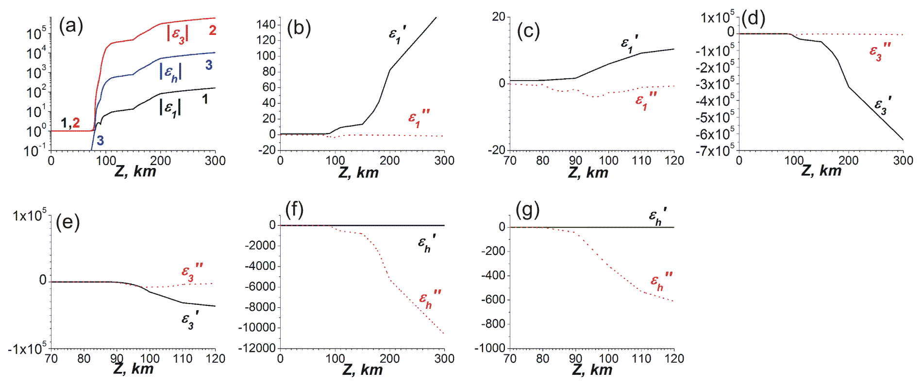
Figure 3 (a) The vertical dependencies of the modules of components of the permittivity in the frame associated with the geomagnetic field $\left|{\mathit{\epsilon }}_{\mathrm{1}}\right|$, $\left|{\mathit{\epsilon }}_{\mathrm{3}}\right|$ and $\left|{\mathit{\epsilon }}_h\right|$ with curves 1, 2 and 3, correspondingly. (b)–(g) The real (corresponding lines with the values denoted by one prime) and imaginary parts (corresponding lines with the values denoted by two primes) of the components ε₁, ε₃ and ε_h in general and detailed views.

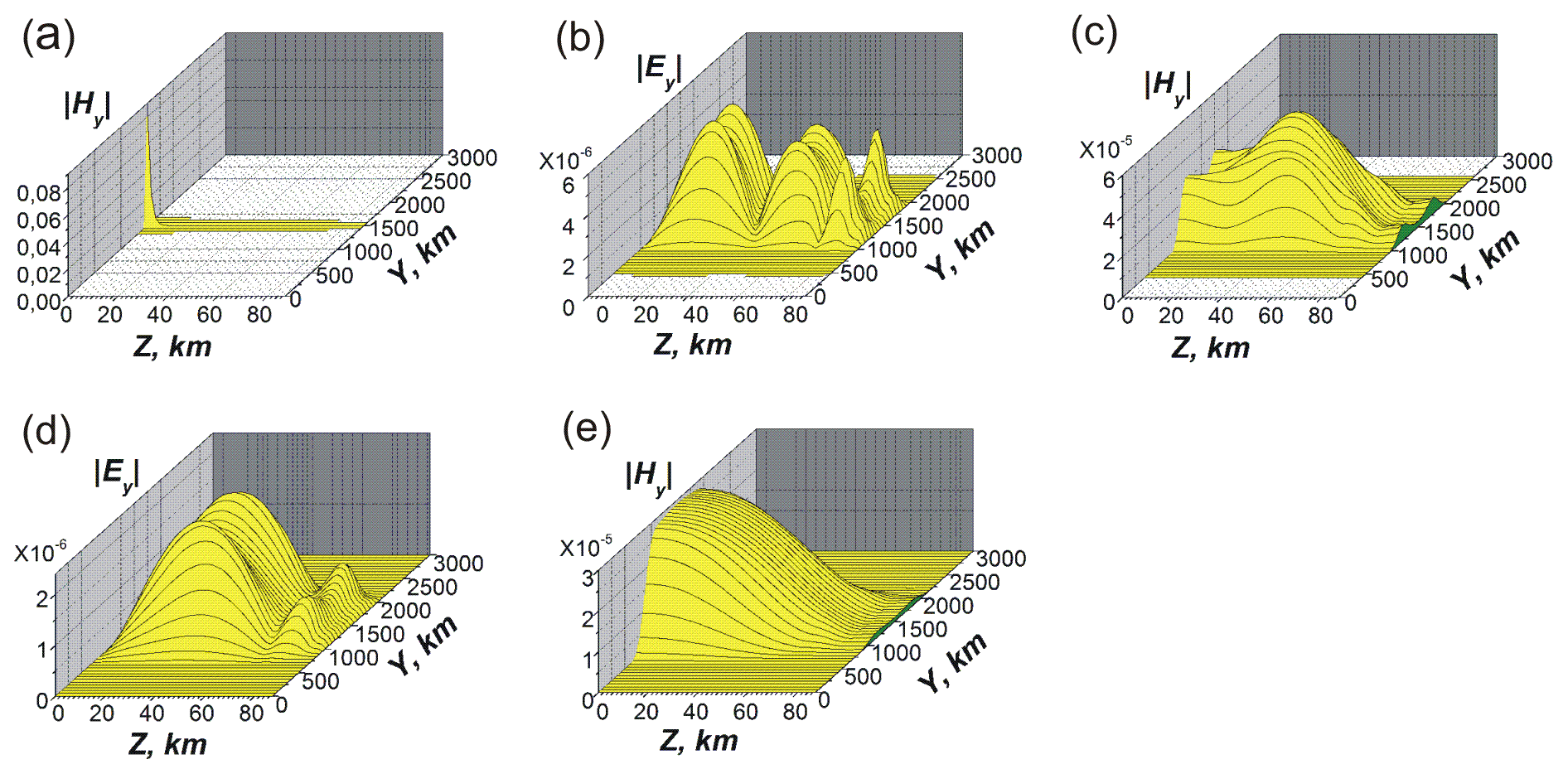
Figure 4 Panel (a) is the initial distribution of $\left|H_y\right|$ at x=0. Panels (b) and (c) are $\left|E_y\right|$ and $\left|H_y\right|$ at x=600 km. Panels (d) and (e) are $\left|E_y\right|$ and $\left|H_y\right|$ at x=1000 km. For the electric field, the maximum value (d) is $\mathrm{3}\times {\mathrm{10}}^{-\mathrm{6}}\mathrm{Gs}\approx \mathrm{1}\mathrm{mV}{\mathrm{cm}}^{-\mathrm{1}}$; for the magnetic field, the maximum value (e) is $\mathrm{3}\times {\mathrm{10}}^{-\mathrm{5}}\mathrm{Gs}\approx \mathrm{3}\mathrm{nT}$. At the altitudes $z<\mathrm{75}\mathrm{km},\left|E_z\right|\approx \left|H_y\right|$. $\mathit{\omega }=\mathrm{1.0}\times {\mathrm{10}}^{\mathrm{5}}{\mathrm{s}}^{-\mathrm{1}}$ and θ=45^∘.

The wave beams are localized within the WGEI at $\mathrm{0}<z<\mathrm{75}\mathrm{km}$, mainly in the regions with the isotropic permittivity (see Fig. 4b–e). The mutual transformations of the beams of different polarizations occur near the waveguide upper boundary due to the anisotropy of the ionosphere within the thin layer at $\mathrm{75}\mathrm{km}<z<\mathrm{85}\mathrm{km}$ (Fig. 4b, d). These transformations depend on the permittivity component values of the ionosphere at the altitude of z>80 km and on the components of the tensor impedance. Therefore, the measurements of the phase and amplitude modulations of different EM components near the Earth's surface can provide information on the properties of the lower and middle ionosphere.

In accordance with boundary condition in Eq. (32), we suppose that when entering the system at X=0, only one of the two polarization modes is excited, namely, the transverse magnetic (TM) mode, i.e., at x=0, H_y≠0 and E_y=0 (Fig. 4a). Upon further propagation of the beam with such boundary conditions at the entrance to the system in a homogeneous isotropic waveguide, the property of the electromagnetic field described by the relation H_y≠0 and E_y=0 will remain valid. The qualitative effect due to the presence of gyrotropy (a) in a thin bulk layer near the upper boundary of WGEI and (b) in the upper boundary condition with complex gyrotropic and anisotropic impedance is as follows: during beam propagation in the WGEI, the transverse electric (TE) polarization mode with the corresponding field components, including E_y, is also excited. This effect is illustrated in Fig. 4b and d.

The magnitude of the E_y component depends on the values of the electron concentration at the altitudes z=75–100 km. In Fig. 5a and b the different dependencies of the electron concentration n(z) are shown (see the solid, dashed and dotted lines 1, 2 and 3, respectively). The corresponding dependencies of the component absolute values of the permittivity are shown in Fig. 4c and d.

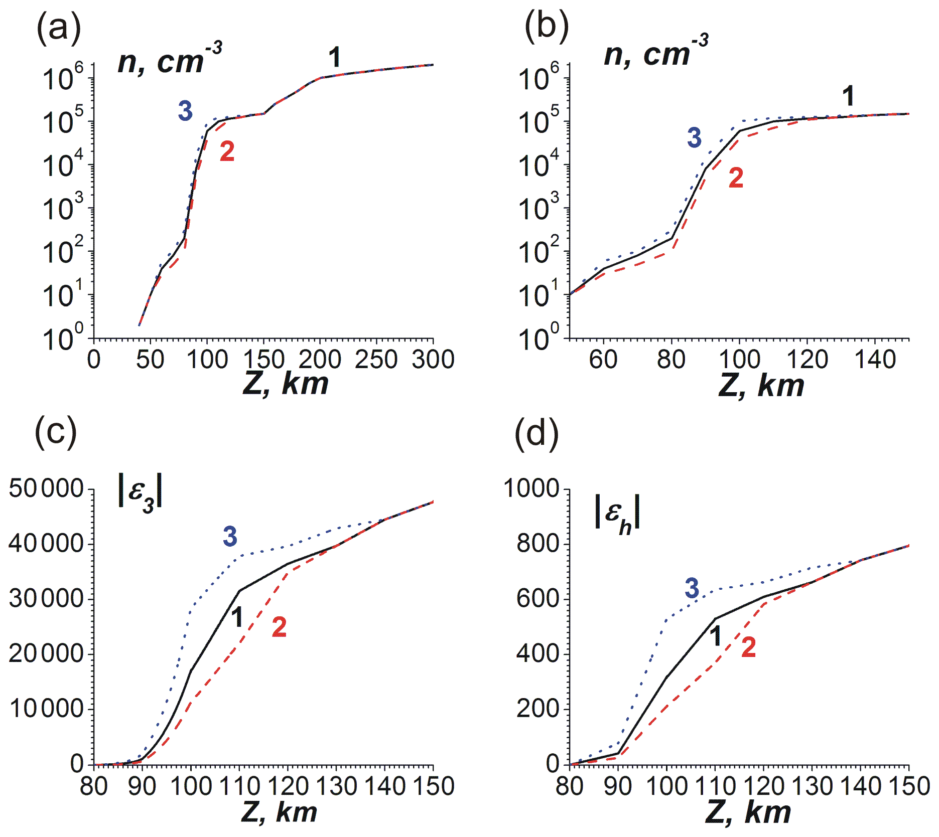
Figure 5 Different profiles of the electron concentration n(z) used in simulations: solid, dashed and dotted lines correspond to undisturbed, decreased and increased concentrations, respectively. Shown are the (a) detailed view and (b) general view. Panels (c) and (d) show the permittivity $\left|{\mathit{\epsilon }}_{\mathrm{3}}\right|$ and ε_h modules.

The distributions of $\left|E_y\right|$ and $\left|H_y\right|$ at x=1000 km are given in Fig. 6. Results in Fig. 6a and b correspond to the solid (1) curve n(z) in Fig. 5; Fig. 6c and d correspond to the dashed (2) curve; Fig. 6e and f correspond to the dotted (3) curve in Fig. 5. The initial H_y beam is the same and is given in Fig. 4a. The values of the tensor impedance for these three cases are presented in Table 1.

Table 1 The values of tensor impedance components corresponding to the data shown in Fig. 5.

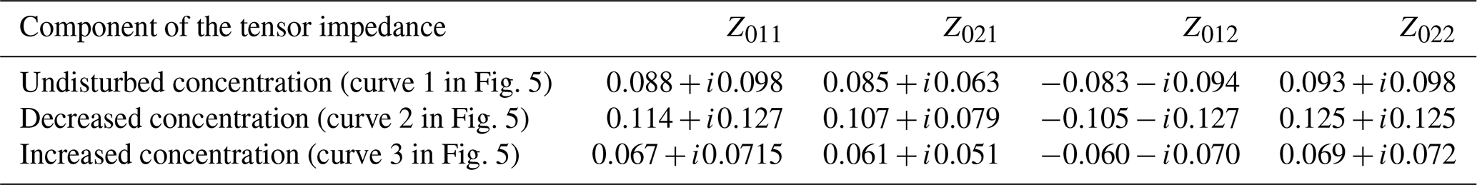
Figure 6 Panels (a), (c) and (e) are dependencies of $\left|E_y\right|$. Panels (b), (d) and (f) are dependencies of $\left|H_y\right|$ at x=1000 km, with $\mathit{\omega }=\mathrm{1.0}\times {\mathrm{10}}^{\mathrm{5}}{\mathrm{s}}^{-\mathrm{1}}$ and θ=45^∘. The initial beams are the same as in Fig. 4a. Panels (a) and (b) correspond to the solid (1) curves in Fig. 5. Panels (c) and (d) are for the dashed (2) curves. Panels (e) and (f) correspond to the dotted (3) curves there.

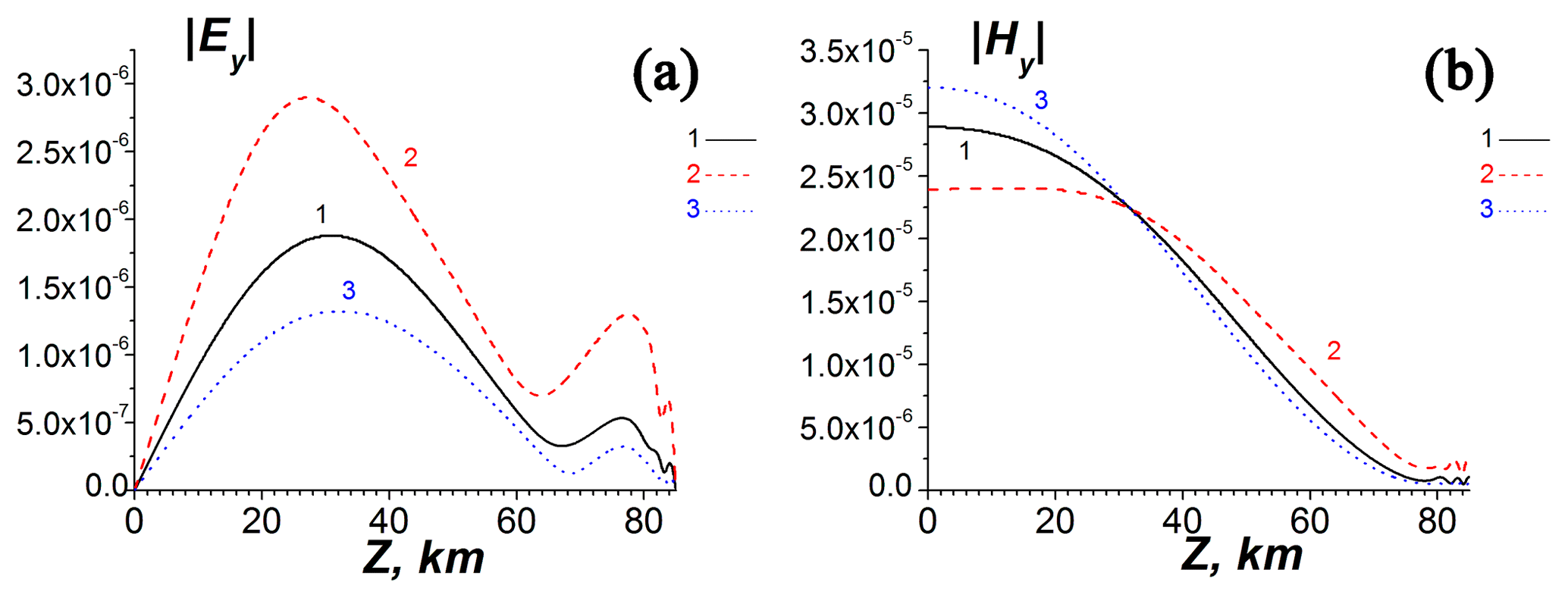
Figure 7 The dependencies of EM components at altitude z in the center of the waveguide at y=1500 km for the different profiles of the electron concentration. The solid (1), dashed (2) and dotted (3) curves correspond to the different profiles of the electron concentration in Fig. 5. Panels (a) and (b) are the same kinds of curves, with $\mathit{\omega }=\mathrm{1.0}\times {\mathrm{10}}^{\mathrm{5}}{\mathrm{s}}^{-\mathrm{1}}$ and θ=45^∘.

The distributions of $\left|E_y\right|$ and $\left|H_y\right|$ on z at x=1000 km in the center of the waveguide, y=1500 km, are given in Fig. 7. These simulations show that the change in the complex tensors of both volume dielectric permittivity and impedance at the lower and upper boundaries of the effective WGEI influence the VLF losses remarkably. The modulation of the electron concentration at the altitudes above z=120 km affects the excitation of the E_y component within the waveguide rather weakly.

5 Influence of the parameters of the WGEI on the polarization transformation and losses of the propagating VLF waves

An important effect of the gyrotropy and anisotropy is the corresponding transformation of the field polarization during the propagation in the WGEI, which is absent in the ideal metal planar waveguide without gyrotropy and anisotropy. We will show that this effect is quite sensitive to the carrier frequency of the beam, propagating in the WGEI, and the inclination of the geomagnetic field and perturbations in the electron concentration, which can vary under the influences of the powerful sources placed below, above and inside the ionosphere. In the real WGEI, the anisotropy and gyrotropy are connected with the volume effect and effective surface tensor impedances at the lower and upper surfaces of the effective WGEI, where z=0 and z=L_z (Fig. 1). For the corresponding transformation of the field polarization determination, we introduce the characteristic polarization relation $|E_y/H_y|(z;y=L_y/\mathrm{2};x=x_{\mathrm{0}})$, taken at the central plane of the beam (y=L_y) at the characteristic distance (x=x₀) from the beam input and VLF transmitter. The choice of the characteristic polarization parameter ($|E_y/H_y|$) and its dependence on the vertical coordinate (z) is justified by conditions (1)–(3). (1) The WGEI is similar to the ideal planar metalized waveguide because, first, the tensor $\widehat{\mathit{ϵ}}$ is different from the isotropic $\widehat{I}$ only in the relatively small upper part of the WGEI in the altitude range from 75–80 to 85 km (see Fig. 1). Second, both the Earth and ionosphere conductivity are quite high, and corresponding impedances are quite low. In particular, the elements of the effective tensor impedance at the upper boundary of the WGEI are small, $\left|Z_{\mathrm{0}\mathit{\alpha }\mathit{\beta }}\right|\le \mathrm{0.1}$ (see, for example, Table 1). (2) Respectively, the carrier modes of the VLF beam are close to the modes of the ideal metalized planar waveguide. These uncoupled modes are subdivided into sets of ($E_x,H_y,E_z$) and ($H_x,E_y,H_z$). The detailed search of the propagation of the separate eigenmodes of the WGEI is not a goal of this paper and will be the subject of the separate paper. (3) Because we have adopted the input boundary conditions in Eq. (32) (with H_y≠0, E_y=0) for the initial beam(s), the above-mentioned value $|E_y/H_y|(z;y=L_y/\mathrm{2};x=x_{\mathrm{0}})$ characterizes the mode coupling and corresponding transformation of the polarization at the distance of x₀ from the beam input due to the presence of the volume and surface gyrotropy and anisotropy in the real WGEI. The results presented below are obtained for x₀=1000 km, that is, by the order of value, a typical distance, for example, between the VLF transmitter and receiver of the European VLF/LF radio network (Biagi et al., 2015). Another parameter characterizing the propagation of the beam in the WGEI is the effective total loss parameter of $\left|H_{y\max }\right(x=x_{\mathrm{0}})/H_{y\max }(x=\mathrm{0}\left)\right|$. Note that this parameter characterizes both dissipative and diffraction losses. The last are connected with beam spreading in the transverse (y) direction during the propagation in the WGEI.

In Fig. 8 the polarization and loss characteristic dependencies on both the carrier beam frequency and the angle θ between the geomagnetic field and the vertical directions (see Fig. 1) are shown.

Figure 8 Characteristics of the polarization transformation parameter $|E_y/H_y|$ (a–c) and the effective coefficient of the total losses at the distance of x₀=1000 km from the beam input (d). Corresponding altitude dependence of the electron concentration is shown in line 1 of Fig. 5b. Panels (a), (b) and (d) show dependences of the polarization parameter (a, b) and total losses (d) on the vertical coordinate and frequency for different θ angles, respectively. Black (1), red (2), green (3) and blue (4) curves in panels (a), (b) and (d) correspond to 5, 30, 45 and 60^∘, respectively. Panels (a) and (b) correspond to the frequencies $\mathit{\omega }=\mathrm{0.86}\times {\mathrm{10}}^{\mathrm{5}}{\mathrm{s}}^{-\mathrm{1}}$ and $\mathit{\omega }=\mathrm{1.14}\times {\mathrm{10}}^{\mathrm{5}}{\mathrm{s}}^{-\mathrm{1}}$, respectively. Panel (c) shows the dependence of the polarization parameter on the vertical coordinate for the different frequencies. Black (1), red (2) and green (3) lines correspond to the frequencies 0.86×10⁵, 1×10⁵ and $\mathrm{1.14}\times {\mathrm{10}}^{\mathrm{5}}{\mathrm{s}}^{-\mathrm{1}}$, respectively, and θ=45^∘.

In Fig. 8a–c the altitude dependence of the polarization parameter $|E_y/H_y|$ exhibits two main maxima in the WGEI. The first one lies in the gyrotropic region above 70 km, while the second one in the isotropic region of the WGEI. As seen from Fig. 8a and b, the value of the (larger) second maximum increases, while the value of the first maximum decreases, and its position shifts to the lower altitudes with increasing frequency. At the higher frequency ($\mathit{\omega }=\mathrm{1.14}\times {\mathrm{10}}^{\mathrm{5}}{\mathrm{s}}^{-\mathrm{1}}$), the larger maximum of the polarization parameter corresponds to the intermediate value of the angle θ=45^∘ (Fig. 8b); for the lower frequency ($\mathit{\omega }=\mathrm{0.86}\times {\mathrm{10}}^{\mathrm{5}}{\mathrm{s}}^{-\mathrm{1}}$), the largest value of the first (higher) maximum corresponds to the almost vertical direction of the geomagnetic field (θ=5^∘; Fig. 8a). For the intermediate value of the angle (θ=45^∘), the largest value of the main maximum corresponds to the higher frequency ($\mathit{\omega }=\mathrm{1.14}\times {\mathrm{10}}^{\mathrm{5}}{\mathrm{s}}^{-\mathrm{1}}$) in the considered frequency range (Fig. 8c). The total losses increase monotonically with increasing frequency and depend weakly on the value of θ (Fig. 8d).

To model the effect of increasing and decreasing the electron concentration n_e in the lower ionosphere on the polarization parameter, we have used the following parameterization for the n_e change $\mathrm{\Delta }{n}_{\mathrm{e}}=n_{\mathrm{e}}\left(z\right)-n_{\mathrm{0}\mathrm{e}}\left(z\right)$ of the electron concentration, where n_0e(z) is the unperturbed altitude distribution of the electron concentration.

$$\begin{array}{}\text{(35)}& \begin{array}{rl}& \mathrm{\Delta }{n}_{\mathrm{e}}\left(z\right)=n_{\mathrm{0}\mathrm{e}}\left(z\right)\mathrm{\Phi }\left(z\right);\\ & \mathrm{\Phi }\left(z\right)=\left[F\right(z\left)\right]-{\displaystyle \frac{(z-z_{\mathrm{2}}{)}^{\mathrm{2}}}{\mathrm{\Delta }{z}_{\mathrm{12}}^{\mathrm{2}}}}\left[F\right(z_{\mathrm{1}}\left)\right]-{\displaystyle \frac{(z-z_{\mathrm{1}}{)}^{\mathrm{2}}}{\mathrm{\Delta }{z}_{\mathrm{12}}^{\mathrm{2}}}}\left[F\right(z_{\mathrm{2}}\left)\right];\\ & F\left(z\right)=f_{\mathrm{00}}\cdot {\cosh }^{-\mathrm{2}}\left\{\left[z-\left({\displaystyle \frac{z_{\mathrm{1}}+z_{\mathrm{2}}}{\mathrm{2}}}\right)\right]/\mathrm{\Delta }z\right\}\end{array}\end{array}$$

In Eq. (35), $\mathrm{\Delta }{z}_{\mathrm{12}}\equiv z_{\mathrm{2}}-z_{\mathrm{1}}$; Δz is the effective width of the electron concentration perturbation altitude distribution. The perturbation Δn_e is concentrated in the range of altitudes $z_{\mathrm{1}}\le z\le z_{\mathrm{2}}$ and is equal to zero outside this region, $\mathrm{\Delta }{n}_{\mathrm{e}}\left(z_{\mathrm{1}}\right)=\mathrm{\Delta }{n}_{\mathrm{e}}\left(z_{\mathrm{2}}\right)=\mathrm{0}$, while $\mathrm{\Phi }\left(z_{\mathrm{1}}\right)=\mathrm{\Phi }\left(z_{\mathrm{2}}\right)=\mathrm{0}$.

Figure 9 (a) Decreased and increased electron concentration (line 2, red) and (line 3, blue) correspond to $f_{\mathrm{00}}=-\mathrm{1.25}$ and f₀₀=250, respectively, relative to the reference concentration (line 1, black) with parametrization conditions (see Eq. 35) z₁=50 km, z₂=90 km and Δ=20 km. Panels (b) and (c) are the polarization parameter $|E_y/H_y|$ altitude distribution for decreased and increased electron concentration, respectively. In (b) and (c) lines 1, 2 and 3 correspond to ω values $\mathrm{0.86}\times {\mathrm{10}}^{\mathrm{5}}{\mathrm{s}}^{-\mathrm{1}}$, $\mathrm{1.0}\times {\mathrm{10}}^{\mathrm{5}}{\mathrm{s}}^{-\mathrm{1}}$ and $\mathrm{1.14}\times {\mathrm{10}}^{\mathrm{5}}{\mathrm{s}}^{-\mathrm{1}}$, respectively. Angle θ is equal to 45^∘.

The change in the concentration in the lower ionosphere causes a rather nontrivial effect on the parameter of the polarization transformation $|E_y/H_y|$ (Fig. 9a–c). Note that either an increase or a decrease in the ionosphere plasma concentration have been reported as a result of seismogenic phenomena, tsunamis, particle precipitation in the ionosphere due to wave–particle interaction in the radiation belts (Pulinets and Boyarchuk, 2005; Shinagawa et al., 2013; Arnoldy and Kintner, 1989; Glukhov et al., 1992; Tolstoy et al., 1986), etc. The changes in the $|E_y/H_y|$ due to an increase or decrease in electron concentration vary by absolute values from dozens to thousands of a percent. This can be seen from the comparison between Fig. 9b and c (lines 3) and Fig. 8c (line 3), which corresponds to the unperturbed distribution of the ionospheric electron concentration (see also lines 1 in Figs. 5b and 9a). It is even more interesting that in the case of decreasing (Fig. 9a, curve 2) electron concentration, the main maximum of $|E_y/H_y|$ appears in the lower atmosphere (at the altitude around 20 km, Fig. 9b, curve 3, which corresponds to $\mathit{\omega }=\mathrm{1.14}\times {\mathrm{10}}^{\mathrm{5}}{\mathrm{s}}^{-\mathrm{1}}$). In the case of increasing electron concentration (Fig. 9a, curve 3), the main maximum of $|E_y/H_y|$ appears near the E region of the ionosphere (at the altitude around 77 km, Fig. 9c). The secondary maximum, which is placed, in the absence of the perturbation of the electron concentration, in the lower atmosphere (Fig. 8c, curves 2 and 3) or mesosphere and ionosphere D region ((Fig. 8c, curve 1) practically disappears or just is not seen in the present scale in the case under consideration (Fig. 9c, curves 1–3).

Figure 10 (a, b) Frequency dependencies of the real (a) and imaginary (b) parts of the effective tensor impedance Z₀₁₁ component at the upper boundary (z=L_z, see Fig. 1) of the WGEI. Lines 1 (black), 2 (red), 3 (blue) and 4 (green) correspond to θ=5, 30, 45 and 60^∘, respectively. Panel (c) shows the polarization parameter $|E_y/H_y|$ altitude dependency at the frequency $\mathrm{0.86}\times {\mathrm{10}}^{\mathrm{5}}{\mathrm{s}}^{-\mathrm{1}}$ and angle θ=45^∘ for the isotropic surface impedance Z₀ at the lower surface of the WGEI equal to 10⁻⁴. Earth conductivity σ is equal to 10⁹ s⁻¹ for line 1 and $Z_{\mathrm{0}}={\mathrm{10}}^{-\mathrm{2}}$ ($\mathit{\sigma }={\mathrm{10}}^{\mathrm{7}}{\mathrm{s}}^{-\mathrm{1}}$) for line 2.

In Fig. 10, the real (a) and imaginary (b) parts of the surface impedance at the upper boundary of the WGEI have a quasi-periodical character with the amplitude of oscillations occurring around the effective average values (not shown explicitly in Fig. 10a and b), which decreases with an increasing angle of θ. The average Re(Z₀₁₁) and Im(Z₀₁₁) values in general decrease with an increasing angle of θ (see Fig. 10a and b). The average values of Re(Z₀₁₁) at θ=5, 30, 45 and 60^∘ (lines 1–4 in Fig. 10a) and Im(Z₀₁₁) at θ=45^∘ and θ=60^∘ (curves 3 and 4 in Fig. 10b) increase with an increasing frequency in the frequency range (0.86–1.14) $\times {\mathrm{10}}^{\mathrm{5}}{\mathrm{s}}^{-\mathrm{1}}$. The average Im(Z₀₁₁) value at θ=5 and 30^∘ changes in the frequency range (0.86–1.14) $\times {\mathrm{10}}^{\mathrm{5}}{\mathrm{s}}^{-\mathrm{1}}$ non-monotonically with the maximum at (1–1.1) $\times {\mathrm{10}}^{\mathrm{5}}{\mathrm{s}}^{-\mathrm{1}}$. The value of finite impedance at the lower Earth–atmosphere boundary of the WGEI influences the polarization transformation parameter minimum near the E region of the ionosphere (lines 1 and 2 in Fig. 10c). The decrease of surface impedance Z₀ at the lower Earth–atmosphere boundary of the WGEI by two orders of magnitude produces the 100 % increase of the corresponding $|E_y/H_y|$ minimum at z∼75 km (Fig. 10c).

6 Discussion

The observations presented in Rozhnoi et al. (2015) show a possibility for seismogenic increasing losses of VLF waves in the WGEI (Fig. 11; see details in Rozhnoi et al., 2015). We discuss the qualitative correspondence of our results to these experimental data.

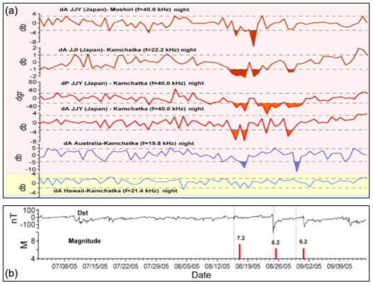
Figure 11 Averaged residual VLF and LF signals from ground-based observations at the wave paths of JJY-Moshiri, JJI-Kamchatka, JJY-Kamchatka, Australia-Kamchatka and Hawaii-Kamchatka. Horizontal dotted lines show the 2σ level. The color-filled zones highlight values exceeding the −2σ level. In panel b Dst (disturbance storm time index) variations and earthquakes magnitude values are shown (from Rozhnoi et al., 2015, see their Fig. 1 but not including the Detection of Electro-Magnetic Emissions Transmitted from Earthquake Regions (DEMETER) data; the work of Rozhnoi et al., 2015, is licensed under a Creative Commons Attribution 4.0 International License (CC BY 4.0)). See other details in Rozhnoi et al. (2015).

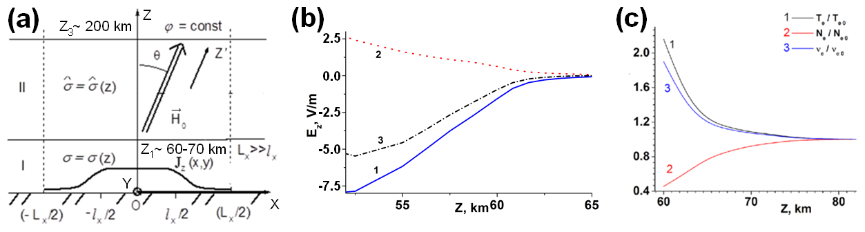
Figure 12 Modification of the ionosphere by the electric field of seismogenic origin based on the theoretical model (Rapoport et al., 2006). (a) Geometry of the model (Rapoport et al., 2006) for the determination of the electric field excited by the seismogenic current source J_z(x,y) and penetrated into the ionosphere with isotropic (I) and anisotropic (II) regions of the “atmosphere–ionosphere” system. (b) Electric field in the mesosphere in the presence of the seismogenic current sources only in the mesosphere (1), in the lower atmosphere (2), and both in the mesosphere and in the lower atmosphere (3). (c) Relative perturbations caused by the seismogenic electric field, normalized on the corresponding steady-state values in the absence of the perturbing electric field, denoted by the index “0”, electron temperature (T_e∕T_e0), electron concentration (N_e∕N_e0) and electron collision frequency (ν_e∕ν_e0).

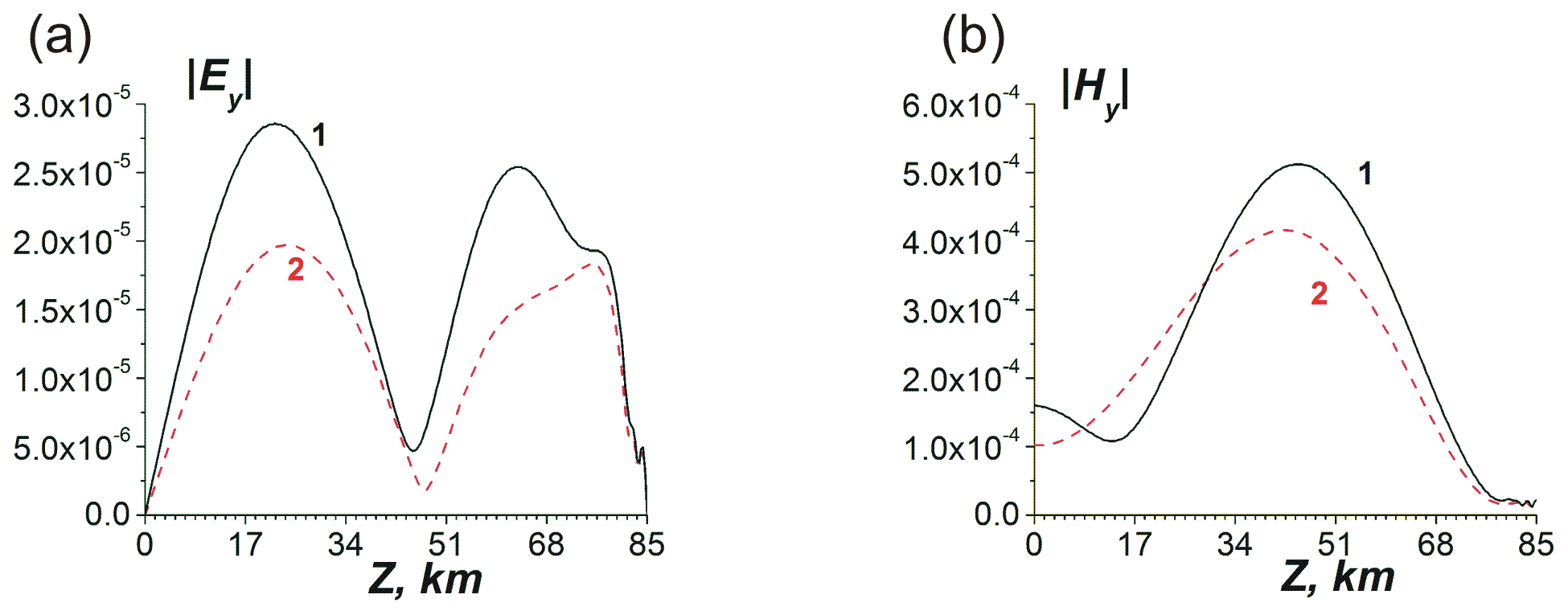
Figure 13 Altitude distributions of the normalized tangential (y) electric (a) and magnetic (b) VLF beam field components in the central plane of the transverse beam distribution (y=0) at the distance of x=1000 km from the input of the system. Line 1 in (a, b) corresponds to the presence of the mesospheric electric current source only with a relatively small value of N_e and a large ν_e. Line 2 corresponds to the presence of both mesospheric and near-ground seismogenic electric current sources with a relatively large value of N_e and small ν_e. Lines 1 and 2 in (a) and (b) correspond qualitatively to the lines 1 and 3, respectively, in Fig. 12b, with $\mathit{\omega }=\mathrm{1.5}\times {\mathrm{10}}^{\mathrm{5}}{\mathrm{s}}^{-\mathrm{1}}$ and θ=45^∘.

The modification of the ionosphere due to electric field excited by the near-ground seismogenic current source has been taken into account. In the model (Rapoport et al., 2006), the presence of the mesospheric current source, which followed from the observations (Martynenko et al., 2001; Meek et al., 2004; Bragin et al., 1974) is also taken into account. It is assumed that the mesospheric current only has the z component and is positive, which means that it is directed vertically downward, as in the fair-weather current (curve 1, Fig. 12b). Then suppose that the surface seismogenic current is directed in the same way as the mesospheric current. We first consider the case when the mesospheric current is zero and only the corresponding seismogenic current is present near the Earth. The corresponding mesospheric electric field under the condition of a given potential difference between the Earth and the ionosphere (curve 2, Fig. 12b) is directed opposite to those excited by the corresponding mesospheric current (curve 1, Fig. 12b). As a result, in the presence of both mesospheric and a seismogenic surface current, the total mesospheric electric field (curve 3, Fig. 12b) is smaller in absolute value than in the presence of only a mesospheric current (curve 1, Fig. 12b). It has been shown by Rapoport et al. (2006) that the decrement of losses $\left|k^{\prime \prime }\right|$ for VLF waves in the WGEI is proportional to $\left|k^{\prime \prime }\right|\sim \left|{\mathit{\epsilon }}^{\prime \prime }\right|\sim N_{\mathrm{e}}/{\mathit{\nu }}_{\mathrm{e}}$. N_e and ν_e decrease and increase, respectively, due to the appearance of a seismogenic surface electric current, in addition to the mesospheric current (curve 3, Fig. 12b). As a result, the losses increase compared with the case when the seismogenic current is absent and the electric field has a larger absolute value (curve 1, Fig. 12). The increase in losses in the VLF beam, shown in Fig. 13 (compare curves 2 and 1 in Fig. 13a and b), corresponds to an increase in losses with an increase in the absolute value of the imaginary part of the dielectric constant when a near-surface seismogenic current source appears (curve 3 in Fig. 12b) in addition to the existing mesospheric current source (curve 2 in Fig. 12b). This seismogenic increase in losses corresponds qualitatively to the results presented in Rozhnoi et al. (2015).

The TIMEB is a new method of modeling characteristics of the WGEI. The results of beam propagation in WGEI modeling presented above include the range of altitudes inside the WGEI (see Figs. 4–7). Nevertheless, the TIMEB method described by Eqs. (15)–(19), (22)–(24), (27), (30a) and (30b) and allows for the determination of all field components in the range of altitudes of $\mathrm{0}\le z\le L_{\max }$, where L_max=300 km. The structure and behavior of these eigenmodes in the WGEI and leakage waves will be a subject of separate papers. We present here only the final qualitative result of the simulations. In the range $L_z\le z\le L_{\max }$, where L_z=85 km is the upper boundary of the effective WGEI, all field components (1) are at least one order of altitude less than the corresponding maximal field value in the WGEI and (2) have the oscillating character along the z coordinate and describe the modes leaking from the WGEI.

Let us make a note also on the dependences of the field components in the WGEI on the vertical coordinate (z). The initial distribution of the electromagnetic field with altitude z (Fig. 4a) is determined by the boundary conditions of the beam (see Eq. 32). The field component includes higher eigenmodes of the WGEI. The higher-order modes experienced quite large losses and practically disappear after beam propagation on a 1000 km distance. This determines the change in altitude (z) and transverse (y) distributions of the beam field during propagation along the WGEI. In particular, at the distance of x=600 km from the beam input (Figs. 4b, c), the few lowest modes of the WGEI along the z and y coordinates still persist. At distance x=1000 km (Figs. 4d, c; 6e, f; and 7a, b), only the main mode persists in the z direction. Note that the described field structure correspond to the real WGEI with losses. The gyrotropy and anisotropy causes the volume effects and surface impedance, in distinction to the ideal planar metalized waveguide with isotropic filling (Collin, 2001).

The closest approach of the direct investigation of the VLF electromagnetic field profile in the Earth–ionosphere waveguide was a series of sounding rocket campaigns at mid and high latitudes at Wallops Island, Virginia, USA, and Siple Station in Antarctica (Kintner et al., 1983; Brittain et al., 1983; Siefring and Kelley, 1991; Arnoldy and Kintner, 1989). Here single-axis E field and three-axis B field antennas, supplemented in some cases with in situ plasma density measurements, were used to detect the far-field fixed-frequency VLF signals radiated by US Navy and Stanford ground transmitters.

The most comprehensive study of the WGEI will be provided by the ongoing NASA VIPER (VLF Trans-Ionospheric Propagation Experiment Rocket) project (PI John Bonnell, University of California, Berkeley; NASA grant no. 80NSSC18K0782). The VIPER sounding rocket campaign consists of a summer nighttime launch during quiet magnetosphere conditions from Wallops Flight Facility, Virginia, USA, collecting data through the D, E and F regions of the ionosphere with a payload carrying the following instrumentation: 2-D E and 3-D H field waveforms (DC-1 kHz); 3-D waveforms ranging from an ELF (extremely low frequency) to VLF (100 Hz to 50 kHz); 1-D wideband E field measurements of plasma and upper hybrid lines (100 kHz to 4 MHz); and Langmuir probe plasma density and ion gauge neutral-density measurements at a sampling rate of at least tens of Hz. The VIPER project will fly a fully 3-D EM field measurement, direct current (DC) through VLF, and relevant plasma and neutral particle measurements at mid latitudes through the radiation fields of (1) an existing VLF transmitter (the very low-frequency shore radio station with the call sign NAA at Cutler, Maine, USA, which transmits at a frequency of 24 kHz and an input power of up to 1.8 MW; see Fig. 11) and (2) naturally occurring lightning transients through and above the leaky upper boundary of the WGEI. This is supported by a vigorous theory and modeling effort in order to explore the vertical and horizontal profile of the observed 3-D electric and magnetic radiated fields of the VLF transmitter and the profile related to the observed plasma and neutral densities. The VLF wave's reflection, absorption and transmission processes as a function of altitude will be searched making use of the data on the vertical VLF E and H field profile.

Figure 14 Proposed VIPER trajectory.

The aim of this experiment will be the investigation of the VLF beams launched by the near-ground source and VLF transmitter with the known parameters and propagating both in the WGEI and leaking from WGEI into the upper ionosphere. Characteristics of these beams will be compared with the theory proposed in the present paper and the theory on leakage of the VLF beams from WGEI, which we will present in the next papers.

7 Conclusions

1. We have developed the new and highly effective robust method of tensor impedance for the VLF electromagnetic beam propagation in the inhomogeneous waveguiding media: the “tensor impedance method for modeling propagation of electromagnetic beams” in a multi-layered and inhomogeneous waveguide. The main differences and advantages of the proposed tensor impedance method in comparison with the known method of impedance recalculating, in particular invariant imbedding methods (Shalashov and Gospodchikov, 2011; Kim and Kim, 2016), are the following: (i) our method is a direct method of the recalculation of tensor impedance, and the corresponding tensor impedance is determined analytically (see Eq. 22); (ii) our method applied for the media without non-locality does not need a solution for integral equation(s), as in the invariant imbedding method; and (iii) the proposed tensor impedance method does not need to reveal the forward and reflected waves. Moreover, even the conditions of the radiation in Eq. (12) at the upper boundary z=L_max are determined through the total field components H_x,y that makes the proposed procedure technically less cumbersome and practically more convenient.

2. The waveguide includes the region for the altitudes $\mathrm{0}<z<\mathrm{80}$–90 km. The boundary conditions are the radiation conditions at z=300 km, which can be recalculated to the lower altitudes as the tensor relations between the tangential components of the EM field. In another words, the tensor impedance conditions have been used at z=80–90 km.

3. The application of this method jointly with the previous results of the modification of the ionosphere by seismogenic electric field gives results which qualitatively are in agreement with the experimental data on the seismogenic increasing losses of VLF wave/beam propagation in the WGEI.

4. The observable qualitative effect is the mutual transformation of different polarizations of the electromagnetic field occur during the propagation. This transformation of the polarization depends on the electron concentration, i.e., the conductivity, of the D and E layers of the ionosphere at altitudes of 75–120 km.

5. Changes in complex tensors of both volume dielectric permittivity and impedances at the lower and upper boundaries of effective the WGEI influence the VLF losses in the WGEI remarkably.

6. An influence is demonstrated on the parameters characterizing the propagation of the VLF beam in the WGEI, in particular, the parameter of the transformation polarization $|E_y/H_y|$ and tensor impedance at the upper boundary of the effective WGEI, the carrier beam frequency, and the inclination of the geomagnetic field and the perturbations in the altitude distribution of the electron concentration in the lower ionosphere.

   • (i)

     The altitude dependence of the polarization parameter $|E_y/H_y|$ has two main maxima in the WGEI: the higher maximum is in the gyrotropic region above 70 km, while the other is in the isotropic region of the WGEI. The value of the (larger) second maximum increases, while the value of the first maximum decreases, and its position shifts to the lower altitudes with increasing frequency. In the frequency range of ω= (0.86–1.14) ×10⁵ s⁻¹, at the higher frequency, the larger maximum polarization parameter corresponds to the intermediate value of the angle θ=45^∘; for the lower frequency, the largest value of the first (higher) maximum corresponds to the nearly vertical direction of the geomagnetic field. The total losses increase monotonically with increasing frequency and depend weakly on the value of θ (Fig. 1).

   • (ii)

     The change in the concentration in the lower ionosphere causes a rather nontrivial effect on the parameter of the polarization transformation $|E_y/H_y|$. This effect does include the increase and decrease of the maximum value of the polarization transformation parameter $|E_y/H_y|$. The corresponding change of this parameter has large values from dozens to thousands of a percent. In the case of a decreasing electron concentration, the main maximum of $|E_y/H_y|$ appears in the lower atmosphere at an altitude of around 20 km. In the case of an increasing electron concentration, the main maximum of $|E_y/H_y|$ appears near the E region of the ionosphere (at the altitude around 77 km), while the secondary maximum practically disappears.

   • (iii)

     The real and imaginary parts of the surface impedance at the upper boundary of the WGEI have a quasi-periodical character with the amplitude of “oscillations” occurring around some effective average value decreases with an increasing angle of θ. Corresponding average values of Re(Z₁₁) and Im(Z₁₁), in general, decrease with an increasing angle of θ. Average values of Re(Z₁₁) for θ equal to 5, 30, 45 and 60^∘ and Im(Z₁₁) correspond to θ equal to 45 and 60^∘, and these increase with an increasing frequency in the considered frequency range of 0.86–1.14 $\times {\mathrm{10}}^{\mathrm{5}}{\mathrm{s}}^{-\mathrm{1}}$. The average value of Im(Z₁₁) corresponds to θ equal to 5 and 30^∘ and changes in the frequency range of 0.86–1.14 $\times {\mathrm{10}}^{\mathrm{5}}{\mathrm{s}}^{-\mathrm{1}}$ non-monotonically while having maximum values around the frequency of 1–1.1 $\times {\mathrm{10}}^{\mathrm{5}}{\mathrm{s}}^{-\mathrm{1}}$.

   • (iv)

     The value of finite impedance at the lower Earth–atmosphere boundary of the WGEI quite observably influences the polarization transformation parameter minimum near the E region of the ionosphere. The decrease of surface impedance Z at the lower Earth–atmosphere boundary of the WGEI in two orders causes the increase of the corresponding minimum value of $|E_y/H_y|$ in ∼100 %.

7. In the range $L_z\le z\le L_{\max }$, where L_z=85 km is the upper boundary of the effective WGEI, all field components (a) are at least one order of altitude less than the corresponding maximal value in the WGEI and (b) have the oscillating character (along the z coordinate), which describes the modes leaking from the WGEI. The detail consideration of the electromagnetic waves leaking from the WGEI will be presented in a separate paper. The initial distribution of the electromagnetic field with z (vertical direction) is determined by the initial conditions on the beam. This field includes higher eigenmodes of the WGEI. The higher-order modes, in distinction to the lower ones, have quite large losses and practically disappear after a beam propagation for 1000 km distance. This circumstance determines the change in altitude (z) distribution of the field of the beam during its propagation along the WGEI. In particular, at the distance of x=600 km from the beam input, the few lowest modes of the WGEI along z coordinates still survived. Further, at x=1000 km, practically, only the main mode in the z direction remains. This fact is reflected in a minimum number of oscillations of the beam field components along z at a given value of x.

8. The proposed propagation of VLF electromagnetic beams in the WGEI model and results will be useful to explore the characteristics of these waves as an effective instrument for diagnostics of the influences on the ionosphere from above in the Sun–solar-wind–magnetosphere–ionosphere system; from below from the most powerful meteorological, seismogenic and other sources in the lower atmosphere and lithosphere and Earth, such as hurricanes, earthquakes and tsunamis; from inside the ionosphere by strong thunderstorms with lightning discharges; and even from far space by gamma flashes and cosmic rays events.

Appendix A: The matrix coefficients included in Eq. (16)

Here the expressions of the matrix coefficients are presented that are used in the matrix factorization to compute the tensor impedance (see Eq. 16).

$$\begin{array}{}\text{(A1)}& \begin{array}{rl}& {\widehat{\mathit{\alpha }}}_N^{\left(\mathrm{0}\right)}=\left(\begin{array}{cc}\mathrm{1}+\frac{i{h}_z}{\mathrm{\Delta }}(k_{\mathrm{1}}-{\mathit{\alpha }}_{\mathrm{1}}{\mathit{\alpha }}_{\mathrm{2}}{k}_{\mathrm{2}});& \frac{i{h}_z}{\mathrm{\Delta }}{\mathit{\alpha }}_{\mathrm{2}}(k_{\mathrm{2}}-k_{\mathrm{1}})\\ \frac{i{h}_z}{\mathrm{\Delta }}{\mathit{\alpha }}_{\mathrm{1}}(k_{\mathrm{1}}-k_{\mathrm{2}});& \mathrm{1}+\frac{i{h}_z}{\mathrm{\Delta }}(k_{\mathrm{2}}-{\mathit{\alpha }}_{\mathrm{1}}{\mathit{\alpha }}_{\mathrm{2}}{k}_{\mathrm{1}})\end{array}\right),{\widehat{\mathit{\alpha }}}_N^{(-)}=\left(\begin{array}{cc}-\mathrm{1};& \mathrm{0}\\ \mathrm{0};& -\mathrm{1}\end{array}\right);\mathrm{\Delta }\equiv \mathrm{1}-{\mathit{\alpha }}_{\mathrm{1}}{\mathit{\alpha }}_{\mathrm{2}};\\ & {\widehat{\mathit{\alpha }}}_j^{(-)}=\left(\begin{array}{cc}(\frac{{\mathit{\beta }}_{\mathrm{22}}}{\mathrm{1}-{\mathit{\beta }}_{\mathrm{22}}\frac{k_x^{\mathrm{2}}}{k_{\mathrm{0}}^{\mathrm{2}}}}{)}_{j-\mathrm{1}/\mathrm{2}};& -(\frac{{\mathit{\beta }}_{\mathrm{21}}}{\mathrm{1}-{\mathit{\beta }}_{\mathrm{22}}\frac{k_x^{\mathrm{2}}}{k_{\mathrm{0}}^{\mathrm{2}}}}{)}_{j-\mathrm{1}/\mathrm{2}}+\frac{i{k}_x{h}_z}{\mathrm{2}}(\frac{{\mathit{\beta }}_{\mathrm{23}}}{\mathrm{1}-{\mathit{\beta }}_{\mathrm{22}}\frac{k_x^{\mathrm{2}}}{k_{\mathrm{0}}^{\mathrm{2}}}}{)}_{j-\mathrm{1}}\\ -(\frac{{\mathit{\beta }}_{\mathrm{12}}}{\mathrm{1}-{\mathit{\beta }}_{\mathrm{22}}\frac{k_x^{\mathrm{2}}}{k_{\mathrm{0}}^{\mathrm{2}}}}{)}_{j-\mathrm{1}/\mathrm{2}}+\frac{i{k}_x{h}_z}{\mathrm{2}}(\frac{{\mathit{\beta }}_{\mathrm{32}}}{\mathrm{1}-{\mathit{\beta }}_{\mathrm{22}}\frac{k_x^{\mathrm{2}}}{k_{\mathrm{0}}^{\mathrm{2}}}}{)}_{j-\mathrm{1}};& ({\mathit{\beta }}_{\mathrm{11}}+\frac{k_x^{\mathrm{2}}}{k_{\mathrm{0}}^{\mathrm{2}}}\frac{{\mathit{\beta }}_{\mathrm{12}}\cdot {\mathit{\beta }}_{\mathrm{21}}}{\mathrm{1}-{\mathit{\beta }}_{\mathrm{22}}\frac{k_x^{\mathrm{2}}}{k_{\mathrm{0}}^{\mathrm{2}}}}{)}_{j-\mathrm{1}/\mathrm{2}}-\\ & -\frac{i{k}_x{h}_z}{\mathrm{2}}({\mathit{\beta }}_{\mathrm{13}}+\frac{k_x^{\mathrm{2}}}{k_{\mathrm{0}}^{\mathrm{2}}}\frac{{\mathit{\beta }}_{\mathrm{12}}\cdot {\mathit{\beta }}_{\mathrm{23}}}{\mathrm{1}-{\mathit{\beta }}_{\mathrm{22}}\frac{k_x^{\mathrm{2}}}{k_{\mathrm{0}}^{\mathrm{2}}}}{)}_{j-\mathrm{1}}-\frac{i{k}_x{h}_z}{\mathrm{2}}({\mathit{\beta }}_{\mathrm{31}}+\frac{k_x^{\mathrm{2}}}{k_{\mathrm{0}}^{\mathrm{2}}}\frac{{\mathit{\beta }}_{\mathrm{32}}\cdot {\mathit{\beta }}_{\mathrm{21}}}{\mathrm{1}-{\mathit{\beta }}_{\mathrm{22}}\frac{k_x^{\mathrm{2}}}{k_{\mathrm{0}}^{\mathrm{2}}}}{)}_j\end{array}\right)\\ & {\widehat{\mathit{\alpha }}}_j^{(+)}=\left(\begin{array}{cc}(\frac{{\mathit{\beta }}_{\mathrm{22}}}{\mathrm{1}-{\mathit{\beta }}_{\mathrm{22}}\frac{k_x^{\mathrm{2}}}{k_{\mathrm{0}}^{\mathrm{2}}}}{)}_{j+\mathrm{1}/\mathrm{2}};& -(\frac{{\mathit{\beta }}_{\mathrm{21}}}{\mathrm{1}-{\mathit{\beta }}_{\mathrm{22}}\frac{k_x^{\mathrm{2}}}{k_{\mathrm{0}}^{\mathrm{2}}}}{)}_{j+\mathrm{1}/\mathrm{2}}-\frac{i{k}_x{h}_z}{\mathrm{2}}(\frac{{\mathit{\beta }}_{\mathrm{23}}}{\mathrm{1}-{\mathit{\beta }}_{\mathrm{22}}\frac{k_x^{\mathrm{2}}}{k_{\mathrm{0}}^{\mathrm{2}}}}{)}_{j+\mathrm{1}}\\ -(\frac{{\mathit{\beta }}_{\mathrm{12}}}{\mathrm{1}-{\mathit{\beta }}_{\mathrm{22}}\frac{k_x^{\mathrm{2}}}{k_{\mathrm{0}}^{\mathrm{2}}}}{)}_{j+\mathrm{1}/\mathrm{2}}-\frac{i{k}_x{h}_z}{\mathrm{2}}(\frac{{\mathit{\beta }}_{\mathrm{32}}}{\mathrm{1}-{\mathit{\beta }}_{\mathrm{22}}\frac{k_x^{\mathrm{2}}}{k_{\mathrm{0}}^{\mathrm{2}}}}{)}_{j+\mathrm{1}};& ({\mathit{\beta }}_{\mathrm{11}}+\frac{k_x^{\mathrm{2}}}{k_{\mathrm{0}}^{\mathrm{2}}}\frac{{\mathit{\beta }}_{\mathrm{12}}\cdot {\mathit{\beta }}_{\mathrm{21}}}{\mathrm{1}-{\mathit{\beta }}_{\mathrm{22}}\frac{k_x^{\mathrm{2}}}{k_{\mathrm{0}}^{\mathrm{2}}}}{)}_{j+\mathrm{1}/\mathrm{2}}+\\ & +\frac{i{k}_x{h}_z}{\mathrm{2}}({\mathit{\beta }}_{\mathrm{13}}+\frac{k_x^{\mathrm{2}}}{k_{\mathrm{0}}^{\mathrm{2}}}\frac{{\mathit{\beta }}_{\mathrm{12}}\cdot {\mathit{\beta }}_{\mathrm{23}}}{\mathrm{1}-{\mathit{\beta }}_{\mathrm{22}}\frac{k_x^{\mathrm{2}}}{k_{\mathrm{0}}^{\mathrm{2}}}}{)}_{j+\mathrm{1}}+\frac{i{k}_x{h}_z}{\mathrm{2}}({\mathit{\beta }}_{\mathrm{31}}+\frac{k_x^{\mathrm{2}}}{k_{\mathrm{0}}^{\mathrm{2}}}\frac{{\mathit{\beta }}_{\mathrm{32}}\cdot {\mathit{\beta }}_{\mathrm{21}}}{\mathrm{1}-{\mathit{\beta }}_{\mathrm{22}}\frac{k_x^{\mathrm{2}}}{k_{\mathrm{0}}^{\mathrm{2}}}}{)}_j\end{array}\right)\\ & {\widehat{\mathit{\alpha }}}_j^{\left(\mathrm{0}\right)}=\left(\begin{array}{cc}-(\frac{{\mathit{\beta }}_{\mathrm{22}}}{\mathrm{1}-{\mathit{\beta }}_{\mathrm{22}}\frac{k_x^{\mathrm{2}}}{k_{\mathrm{0}}^{\mathrm{2}}}}{)}_{j-\mathrm{1}/\mathrm{2}}-(\frac{{\mathit{\beta }}_{\mathrm{22}}}{\mathrm{1}-{\mathit{\beta }}_{\mathrm{22}}\frac{k_x^{\mathrm{2}}}{k_{\mathrm{0}}^{\mathrm{2}}}}{)}_{j+\mathrm{1}/\mathrm{2}}+k_{\mathrm{0}}^{\mathrm{2}}{h}_z^{\mathrm{2}};& (\frac{{\mathit{\beta }}_{\mathrm{21}}}{\mathrm{1}-{\mathit{\beta }}_{\mathrm{22}}\frac{k_x^{\mathrm{2}}}{k_{\mathrm{0}}^{\mathrm{2}}}}{)}_{j-\mathrm{1}/\mathrm{2}}+(\frac{{\mathit{\beta }}_{\mathrm{21}}}{\mathrm{1}-{\mathit{\beta }}_{\mathrm{22}}\frac{k_x^{\mathrm{2}}}{k_{\mathrm{0}}^{\mathrm{2}}}}{)}_{j+\mathrm{1}/\mathrm{2}}\\ (\frac{{\mathit{\beta }}_{\mathrm{12}}}{\mathrm{1}-{\mathit{\beta }}_{\mathrm{22}}\frac{k_x^{\mathrm{2}}}{k_{\mathrm{0}}^{\mathrm{2}}}}{)}_{j-\mathrm{1}/\mathrm{2}}+(\frac{{\mathit{\beta }}_{\mathrm{12}}}{\mathrm{1}-{\mathit{\beta }}_{\mathrm{22}}\frac{k_x^{\mathrm{2}}}{k_{\mathrm{0}}^{\mathrm{2}}}}{)}_{j+\mathrm{1}/\mathrm{2}};& -({\mathit{\beta }}_{\mathrm{11}}+\frac{k_x^{\mathrm{2}}}{k_{\mathrm{0}}^{\mathrm{2}}}\frac{{\mathit{\beta }}_{\mathrm{12}}\cdot {\mathit{\beta }}_{\mathrm{21}}}{\mathrm{1}-{\mathit{\beta }}_{\mathrm{22}}\frac{k_x^{\mathrm{2}}}{k_{\mathrm{0}}^{\mathrm{2}}}}{)}_{j-\mathrm{1}/\mathrm{2}}-({\mathit{\beta }}_{\mathrm{11}}+\frac{k_x^{\mathrm{2}}}{k_{\mathrm{0}}^{\mathrm{2}}}\frac{{\mathit{\beta }}_{\mathrm{12}}\cdot {\mathit{\beta }}_{\mathrm{21}}}{\mathrm{1}-{\mathit{\beta }}_{\mathrm{22}}\frac{k_x^{\mathrm{2}}}{k_{\mathrm{0}}^{\mathrm{2}}}}{)}_{j+\mathrm{1}/\mathrm{2}}+\\ & +k_{\mathrm{0}}^{\mathrm{2}}{h}_z^{\mathrm{2}}\cdot (\mathrm{1}-{\mathit{\beta }}_{\mathrm{33}}\frac{k_x^{\mathrm{2}}}{k_{\mathrm{0}}^{\mathrm{2}}}-\frac{k_x^{\mathrm{4}}}{k_{\mathrm{0}}^{\mathrm{4}}}\frac{{\mathit{\beta }}_{\mathrm{23}}\cdot {\mathit{\beta }}_{\mathrm{32}}}{\mathrm{1}-{\mathit{\beta }}_{\mathrm{22}}\frac{k_x^{\mathrm{2}}}{k_{\mathrm{0}}^{\mathrm{2}}}}{)}_j\end{array}\right)\end{array}\end{array}$$