the Creative Commons Attribution 4.0 License.
the Creative Commons Attribution 4.0 License.
 | 06 Feb 2020
Observing geometry effects on a Global Navigation Satellite System (GNSS)-based water vapor tomography solved by least squares and by compressive sensing
Marion Heublein
Patrick Erik Bradley
Stefan Hinz
In this work, the effect of the observing geometry on the tomographic reconstruction quality of both a regularized least squares (LSQ) approach and a compressive sensing (CS) approach for water vapor tomography is compared based on synthetic Global Navigation Satellite System (GNSS) slant wet delay (SWD) estimates. In this context, the term “observing geometry” mainly refers to the number of GNSS sites situated within a specific study area subdivided into a certain number of volumetric pixels (voxels) and to the number of signal directions available at each GNSS site. The novelties of this research are (1) the comparison of the observing geometry's effects on the tomographic reconstruction accuracy when using LSQ or CS for the solution of the tomographic system and (2) the investigation of the effect of the signal directions' variability on the tomographic reconstruction. The tomographic reconstruction is performed based on synthetic SWD data sets generated, for many samples of various observing geometry settings, based on wet refractivity information from the Weather Research and Forecasting (WRF) model. The validation of the achieved results focuses on a comparison of the refractivity estimates with the input WRF refractivities. The results show that the recommendation of Champollion et al. (2004) to discretize the analyzed study area into voxels with horizontal sizes comparable to the mean GNSS intersite distance represents a good rule of thumb for both LSQ- and CS-based tomography solutions. In addition, this research shows that CS needs a variety of at least 15 signal directions per site in order to estimate the refractivity field more accurately and more precisely than LSQ. Therefore, the use of CS is particularly recommended for water vapor tomography applications for which a high number of multi-GNSS SWD estimates are available.
- Article
(6262 KB) - Full-text XML
- BibTeX
- EndNote


In this paper, we intend to determine the three-dimensional (3-D) atmospheric water vapor distribution for each point in time. This adds further essential information to the spatio-temporal analyses of two-dimensional (2-D) water vapor fields commonly used in weather forecasting and climate research. In addition, atmospheric water vapor delays the microwave signal propagation within the atmosphere and thus represents an error source in, e.g., Global Navigation Satellite System (GNSS) and Interferometric Synthetic Aperture Radar (InSAR) observations. Therefore, a precise knowledge of the water vapor field, for example, is required for accurate deformation monitoring using InSAR (Hansen and Yu, 2001). However, the atmospheric water vapor distribution is difficult to model because it is highly variable in time and space. Several approaches exist for reconstructing the 3-D tomographic water vapor reconstruction using one-dimensional (1-D) GNSS slant wet delays (SWDs); see Sect. 2.
One of the main limiting factors in water vapor tomographies consists of the point-wise GNSS observing geometry, which causes an ill-conditioned inverse tomographic model that needs to be regularized. Yet, even after regularization, the observing geometry composed, e.g., of the number and the geographic distribution of the GNSS sites, the SWD signal directions, and the voxel discretization still affect the quality of the tomographic solution. This work therefore meets the challenge of comparing the observing geometry's effect on a GNSS-based water vapor tomography solved by means of least squares (LSQ) or by means of compressive sensing (CS). By investigating the observing geometry's effect on the LSQ and CS solution strategies, the differences between the LSQ solution and a CS solution approach benefiting from the signal's sparsity in an appropriate transform domain for regularization are better understood, and recommendations can be given for future water vapor tomography campaigns and the processing of their measurements. Based on synthetic data sets deduced from the Weather Research and Forecasting (WRF) model described in Skamarock et al. (2005), the presented work answers the research question of (1) to what extent the rule of thumb of Champollion et al. (2004), derived for LSQ and recommending a voxel size corresponding to the mean GNSS intersite distance, can be transferred from an LSQ solution to a CS solution. In addition, this research investigates (2) in which settings CS is able to more accurately and more precisely reconstruct the tomographic water vapor field than LSQ and (3) to what extent multi-GNSS SWD observations improve the tomographic solution obtained by means of LSQ or CS when compared to solutions obtained from SWDs originating from the Global Positioning System (GPS) only.
Current water vapor tomographies can be distinguished, e.g., based on the methodology and the data sets applied for solving the tomographic model. The tomographic model is commonly established based on the directions along which space-geodetic SWD estimates are acquired and based on a discretization of the investigated atmospheric volume into volumetric pixels (voxels), e.g., of constant refractivity. The existing tomography solution approaches applied to such a discretized atmosphere are subdivided into iterative and non-iterative techniques. Bender et al. (2011a) propose different iterative algebraic reconstruction techniques (ARTs), while Hirahara (2000), Flores et al. (2000), Champollion et al. (2004), Troller (2004), Song et al. (2006), Notarpietro et al. (2008), and Rohm (2013) apply different non-iterative methods for solving the tomographic system using an LSQ adjustment. Thanks to its good capability to estimate dynamically changing parameters, Flores et al. (2000), Gradinarsky and Jarlemark (2004), and Rohm et al. (2014) choose a Kalman filter approach. Hirahara (2000) proposes a damped least squares solution known from seismic tomography to solve the tomographic problem. Xia et al. (2013) combine iterative and non-iterative techniques. Instead of using voxels in water vapor tomographies with a small number of GNSS sites, Ding et al. (2018) discretize the tomographic field based on the perimeter of the tomographic boundary on the plane and based on meshing techniques. They then determine tomographic fields by means of fitting the real distribution of GNSS signals on different tomographic planes at different tomographic epochs.
In addition to slant wet delay estimates from the GNSS, Hurter and Maier (2013) introduce wet refractivity profiles from radio occultation and radiosonde observations into a combined least squares collocation. Rather than using slant wet delay estimates as input observations, Nilsson and Elgered (2007) apply a solution that relies directly on GPS phase observations.
Independently of the reconstruction strategy, due to the point-wise GNSS observing geometry, the tomographic system of equations is usually ill posed and needs to be regularized, e.g., (i) by constraining the tomographic system by means of pseudo observations, (ii) by introducing additional observations from models, from simulations, or from other sensors, or (iii) by decreasing the number of voxels crossed by no rays at all.
Both Flores et al. (2000) and Gradinarsky and Jarlemark (2004) regularize the solution by means of adding horizontal and vertical smoothing constraints to the tomographic system and by means of introducing a boundary constraint assuming the refractivity to approach zero above a certain height. Alternatively, as proposed in Elosegui et al. (1998), the refractivity field can be assumed to decrease exponentially with increasing height. Yet, while regularizing the solution significantly, both geometric constraints and the exponential decay usually are not able to accurately model the real atmospheric state. As an alternative to using horizontal and vertical constraints relying on physical approximations to the atmospheric behavior, the work in Heublein et al. (2018) and Heublein (2019) exploits the signal's sparsity in a particular, predefined transform domain as prior knowledge for regularizing the tomographic system in order to then reconstruct the signal using an L1-norm minimization. Similarly, CS and sparse reconstruction are applied here for the tomographic reconstruction of the 3-D water vapor field, and the CS solution to water vapor tomography is compared to a solution obtained using a classical LSQ approach. Initially presented by Candès (2006), Donoho (2006), Baraniuk (2007), and Candès and Wakin (2008) for the image or signal recovery from a number of samples below the desired resolution or the Nyquist rate, CS has been, since then, applied to many remote sensing problems in which sparse signals occur. For example, Potter et al. (2010) and Alonso et al. (2010) describe the use of CS for synthetic aperture radar (SAR) imaging, Pruente (2010) applies CS for ground-moving target identification, Zhu and Bamler (2010), Budillon et al. (2011), Aguilera et al. (2013), and Zhu and Bamler (2014) apply CS to SAR tomography, and Li and Yang (2011), Zhu and Bamler (2013), Grohnfeldt et al. (2013), Jiang et al. (2014), and Zhu et al. (2016) use CS for pan-sharpening and hyperspectral image enhancement. When compared to classical LSQ adjustments usually applying L2-norm regularizations, compressive sensing and sparse reconstruction based on a small number of measurements led to promising results.
However, compressive sensing only yields encouraging results if the input data acquisition – corresponding, in water vapor tomography, to the determination of SWD estimates – fulfills certain prerequisites. For general applications of CS, Rauhut (2010), e.g., states that randomness in the acquisition step helps in utilizing the minimum number of measurements. When reconstructing images based on frequency data, Candès (2006), e.g., alternatively recommend randomly measuring frequency coefficients such that sparse objects are sensed by taking as few measurements as possible. For CS-based water vapor tomography approaches, no explicit requirements for acquiring the SWD or for designing advantageous observing geometry settings have been established so far.
For LSQ, Champollion et al. (2004) state that the optimal horizontal size of a voxel should correspond to the mean intersite distance between the used GNSS sites. Given a certain cutoff elevation angle, the height layers' thicknesses in their approach should be defined such that signals received at a GNSS site situated within a voxel's center are able to cross neighboring voxels. Due to the small wet refractivity values in the upper layers and in order to make the tomographic solutions less sensitive to errors in the input data, Rohm (2012) recommends increasing the height layer thicknesses with increasing altitude. Bender and Raabe (2007) and Bender et al. (2009) estimate the spatial distribution of the geometric intersection points between different ray paths in order to compute the information density contained in a given set of GPS signals. They then use this information as a precondition for an optimal tomographic reconstruction and in order to identify regions that are well covered by GPS slant paths. Although Bender et al. (2011b) and Zhao et al. (2019) state that changing the observing geometry by combining multi-GNSS observations instead of GPS-only observations does not substantially improve the reconstruction quality, Rohm (2012) realizes that the uncertainty of the tomographic solution is largely influenced by the mathematical properties of the design matrix, depending itself on the observing geometry. With the aim of giving advice for the installation of new permanent sites and for the solution of future water vapor tomographies, this work therefore investigates the observing geometry's effect on the quality of both an LSQ solution and a CS solution to the tomographic system.
In order to analyze the observing geometry's effect on the quality of the LSQ and CS solutions to water vapor tomography, different observing geometry settings are defined. Based on synthetic SWD estimates derived from WRF, 3-D water vapor distributions are reconstructed for each of the defined observing geometry settings using both LSQ and CS. The quality of the LSQ and CS solutions to water vapor tomography is then compared with respect to the respective observing geometry settings.
3.1 Tomographic model
For tomography using GNSS SWDs, Flores et al. (2000) introduce the functional model
where SWDi, cont stands for the integrated slant wet delay observations between a certain satellite and a certain GNSS site and dl is a differential along the slant ray path. As in Heublein et al. (2018) and Heublein (2019), the variable spi is the ith slant ray path, i.e., the slant ray path of the radio-wave signal between a certain satellite and a certain receiver. The variable Nwet contains the wet refractivity along this path. The index i attains the values
where N corresponds to the number of observations available between any receiver and any satellite. When tomographically reconstructing the wet refractivity, however, the continuous functional model from Eq. (1) is usually replaced by a discrete functional model:
That is, the 3-D water vapor distribution is discretized into voxels in longitude, latitude, and height, assuming a constant refractivity value for each voxel. As in Heublein et al. (2018) and Heublein (2019), in this work, a uniform voxel discretization is selected in the horizontal directions, while the voxel sizes in the vertical direction increase with increasing height. Horizontally, the voxels are limited by constant longitudes and latitudes. In the vertical direction, the voxels are separated by layers of constant ellipsoidal height.
As in Heublein et al. (2018) and Heublein (2019), summarizing all observations SWDi, disc in an observation vector , all unknown refractivities Nwet j for
in a parameter vector , and all distances dij in a design matrix , the discrete tomographic system from Eq. (3) can be rewritten as
with
As each signal only passes a small subsection of the study area, most entries of the matrix Φdata are zero and only a few matrix elements are non-zero (e.g., only about 5 % of the entries of Φdata are non-zero in the case of an about 95×99 km2 large study area subdivided into voxels, consisting of seven GNSS sites and 10 signals per site). For voxels that are not crossed by any signals, Φdata has a zero column. Therefore, the tomographic model and the mathematical properties of the design matrix largely depend on the observing geometry settings described in Sect. 3.3.
3.2 Solution of the inverse tomographic model using LSQ or CS
The LSQ solution to Eq. (5) is derived by solving the minimization problem
regularized by means of t=3 regularization terms, namely by horizontal and vertical smoothing constraints as well as by prior knowledge from surface meteorology. That is, the wet refractivity at the surface is computed from in situ observations of pressure, temperature, and dew point temperature at a single weather site within the study area. As described in Heublein et al. (2018), the horizontal smoothing constraints assuming the refractivity of a voxel to equal the weighted mean refractivity of the surrounding voxels with voxel indices p≠a and q≠b within the same height layer k are defined by
The weights can, e.g., be derived using inverse distance weighting:
with distances between the center of voxel (p,q) and the center of voxel (a,b) of the considered kth height layer.
Moreover, Davis et al. (1993) state that an average refractivity profile can be approximated assuming the refractivity to exponentially decrease with height:
The variable hk is the height of the kth layer, h0 stands for some reference height at which the refractivity equals Nwet(h0), and Hscale represents the scale height of the local troposphere. As Hscale is essential for defining an exponential decay with height, its value is determined within the solution of the tomographic system from a set of realistic values for Hscale between 1000 and 2000 m. Both the weights for the horizontal and vertical smoothing constraints and for the prior knowledge from surface meteorology are determined with respect to the data fidelity term using the place holder trade-off parameter in Eq. (7). The selection of the trade-off parameters from a certain number of logarithmically scaled possible trade-off parameters and the selection of Hscale are described in Heublein et al. (2018) and Heublein (2019).
When aiming at a tomographic reconstruction of atmospheric water vapor by means of compressive sensing, the parameters x are sparsely represented in some transform domain
as sparse parameters s. Estimates for these sparse parameters are obtained by
as described in Heublein et al. (2018) and Heublein (2019). Instead of adding horizontal and vertical constraints to the data fidelity term as in Eq. (7), an L1-norm regularization term is introduced into the CS solution to promote sparse solutions for s, as described in Heublein et al. (2018) and Heublein (2019). The L1-norm minimization of the sparse parameters reduces the solution space. The wet refractivity estimates are then reconstructed using
with a dictionary . As in Heublein et al. (2018) and Heublein (2019), the dimension M of the parameters in the transform domain varies with the number of base functions or atoms in Ψ. Similarly to Heublein et al. (2018) and Heublein (2019), we assert that a sparse representation of the refractivity distribution can be obtained by means of, e.g., a dictionary composed of Kronecker products of inverse discrete cosine transform (iDCT) letters in longitudinal and latitudinal directions and of Euler letters and Dirac letters in the height direction. When thinking of languages, an atom would stand for a word within a dictionary. Comparably to a word composed of different letters within a language dictionary, each atom results from the Kronecker product of smaller items, namely letters, within the dictionary for sparse representation. That is, for each column, i.e., line, of the 3-D wet refractivity signal, a Kronecker product of the 1-D letters along the longitudinal, latitudinal, and height directions is computed. In the longitudinal and latitudinal directions, iDCT letters will represent horizontal refractivity variations. The Euler letters model an exponential refractivity decay with height, and the Dirac letters describe deviations from a decay described by a linear combination of Euler letters.
3.3 Characteristics of the study area and observing geometry settings
In Sect. 4, tomographic solutions obtained based on a high number of different observing geometry settings are compared. The observing geometry settings result from (i) a fixed voxel discretization, (ii) 7 to 32 sites, (iii) 5 to 20 signal directions per site, and (iv) 48 signal direction samples per number of sites and signals. Champollion et al. (2004) recommend (i) horizontal voxel sizes for an LSQ solution to water vapor tomography greater than or equal to the mean intersite distance between the available GNSS sites, i.e., voxel sizes greater than or equal to about 37×37 km2 or to about 17×17 km2 in the case of 7 or 32 uniformly distributed GNSS sites within the investigated study area of about 95×99 km2 in size. In this work, the study area is discretized into voxels of horizontal sizes of about 19×20 km2. In the vertical direction, five height layers are distinguished. With increasing height, the height layer thicknesses increase from 1300 up to 2900 m. The lowest layer's thickness is set to 1300 m in order to ensure at least for signals with very low elevation angles that a signal arriving at the center of a voxel is able to pass the horizontally neighboring voxel within the same height layer. This is only possible if the minimum thickness Δdlmin of the height layers is related to the horizontal voxel size Δhz=20 km and to the cutoff elevation angle ϵcut=7∘ by means of
The (ii) minimum number of seven sites originates from the real GNSS Upper Rhine Graben (URG) network site distribution within the analyzed study area. The maximum number of sites is chosen such that the rule of thumb of Champollion et al. (2004), introduced in Sect. 2, is clearly fulfilled. The horizontal position of the synthetic GNSS sites corresponds, for seven sites, to the position of real GNSS sites within the analyzed study area. The horizontal position of the additionally defined synthetic GNSS sites is chosen such that they are uniformly distributed within the study area. The vertical position of the synthetic GNSS sites corresponds to the height of the WRF digital elevation model at the horizontal position of the sites. The (iii) number of signal directions per site is motivated by the GPS or by a multi-GNSS orbit geometry. According to Feairheller and Clark (2006), the Global'naya Navigatsionnaya Sputnikova Sistema (GLONASS) constellation consists of 21 active plus 3 spare satellites on three orbital planes inclined by 64.8∘ with respect to the Equator. In contrast, Hofmann-Wellenhof et al. (2008) describe the GPS orbit constellation as consisting of 21 satellites plus 3 spares on six orbital planes inclined by 55∘ with respect to the Equator and the Galileo orbit constellation as consisting of 27 operational plus 3 spare satellites on three planes inclined by 56∘ with respect to the Equator. Therefore, five signal directions and five visible satellites correspond to a pessimistic GPS setting, e.g., with site-specific shadowing. Eight signal directions per site are here considered to be a typical GPS setting at a GNSS permanent site (there may even be up to 12 observations for GPS-only), at which about 30 % of the total number of GPS satellites is visible at a time. Similarly, a total number of 20 signal directions per site corresponds to a visibility of about 30 % of the total number of satellites at a time within a multi-GNSS constellation composed of GPS, GLONASS, and Galileo. Similarly, observation of the BeiDou Navigation Satellite System could also be used in order to increase the number of signal directions in tomography applications. For each of the mentioned numbers of sites and numbers of visible satellites, 48 signal direction samples are defined. Given the GPS repeat cycle of about 1 d, the number of 48 signal direction samples is chosen in order to emulate about half-hourly orbit samples. Using the orbit characteristics mentioned above, such synthetic half-hourly satellite positions are approximated by means of circular orbits.
For each of the described observing geometry settings, synthetic SWD observations as input for the tomographic system are deduced from one single WRF simulation covering an about 200 km × 200 km large area centered around the longitude and latitude (λ, φ) = (8.15, 49.15∘) at a 900 m horizontal resolution. The vertical resolution increases with height, ranging from about 50 to about 500 m. As schematically illustrated in Fig. 1, for each synthetic GNSS site, this is done by means of averaging the refractivity information of all WRF cells situated within the defined tomographic voxels, a direct ray tracing within these tomographic voxels, and adding together the SWD along each signal direction within the tomographic voxels using Eq. (3). As the voxels are limited by ellipsoidal upper and lower borders, the ray tracing is performed according to Perler (2011).
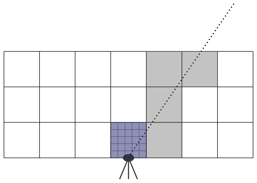
Figure 1Schematic illustration of the generation of synthetic GNSS SWDs according to Heublein (2019): within each tomographic voxel (grey), the WRF refractivities of all those WRF cells (blue) situated within that voxel are averaged. A direct ray tracing along the considered signal direction then yields the SWD introduced into the tomographic system.
The horizontal distribution of the synthetic GNSS sites within the URG study area is shown in Fig. 2. The signal directions result from selecting at random the defined number of signal directions from a synthetic multi-GNSS orbit constellation composed of GPS, GLONASS, and Galileo. Both signals entering the study area at its top and on its side are included.
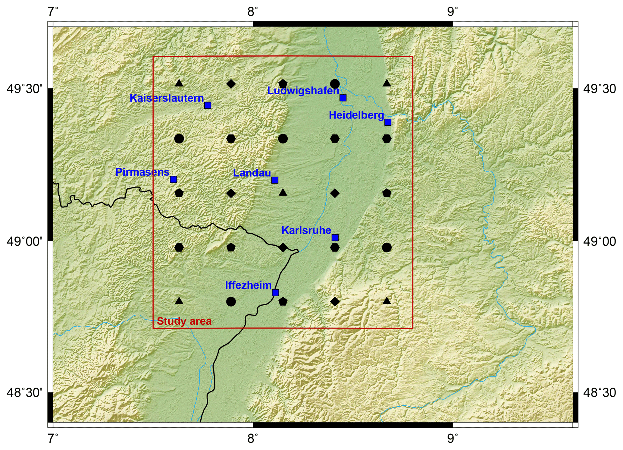
Figure 2Distribution of the 7 GNSS permanent sites (blue squares) as well as of the 5 to 25 additional, synthetic sites (black symbols) within the URG study area. The additional, synthetic sites are distributed within a grid that uniformly covers the study area. Triangles, pentagons, hexagons, diamonds, and circles represent the first, second, third, fourth, and fifth group of five additional sites each.
From WRF, simulations of water vapor mixing ratio, temperature, pressure, and geopotential height are available at a 900 m horizontal resolution for generating the synthetic GNSS SWDs within the 95×99 km2 large study area situated in the URG as shown in Fig. 2. The topography within the Rhine Valley is flat. Height differences mainly occur at the foot of the Black Forest mountain range. The height difference between the highest and lowest synthetic GNSS sites used for this study is about 494 m.
For the most humid acquisition date (27 June 2005) for which WRF simulations were provided for this research and for an exemplary voxel in the lower middle of the lowest voxel layer, Fig. 3 shows that variations in the SWD signal directions available within the tomographic system cause variations in the estimated refractivities. The magnitudes of the absolute wet refractivity values during the analyzed weather conditions range from 0 to 74 ppm. As variations in the signal directions imply a change in the observed atmospheric volume, these variations in the estimated refractivities seem obvious. Yet, Fig. 3 illustrates that the variations in the refractivity estimates vary with the selected solution strategy. When considering many sites and many signal directions per site (e.g., at least 27 sites and at least 15 signal directions), the difference between the CS refractivity estimates and the WRF refractivity of the considered voxel approaches zero for most samples. However, e.g., for 27 sites and 20 signal directions per site, there are some samples in which the CS-based refractivity estimate differs from the WRF refractivity by up to 3.3 ppm. That is, for many signal directions, CS is able to accurately and precisely reconstruct the voxel's refractivity, but for some signal directions, the voxel's refractivity estimate does not match well with the voxel's validation refractivity from WRF. In contrast, in the case of few sites and few signal directions per site (e.g., 12 sites and 10 signal directions per site), LSQ yields refractivity estimates differing from −5.9 to −0.7 ppm from the WRF refractivity, while the CS refractivity estimates differ much more from the WRF refractivity (differences of −42.9 to 26.9 ppm). Consequently, when investigating the observing geometry's effect on the quality of the tomographic reconstruction, the chosen solution strategy as well as the effect of varying signal directions should be taken into account. Therefore, in this research, a representative set of 48 half-hourly samples of synthetic GNSS orbits is considered in order to analyze the observing geometry's effect on the tomographic reconstruction quality.

Figure 3Absolute differences between estimated refractivity and the WRF refractivity in ppm for an exemplary voxel in the lower middle of the lowest voxel layer for the 48 samples of each investigated observing geometry setting. The two left columns use an ordinate ranging from −25 to 25 ppm, the third column plots the differences within the range −10 to 10 ppm, and the right column plots the differences within the range −5 to 5 ppm. The legend in the upper left subplot holds for all the subplots: red circles stand for the LSQ results, while blue squares represent the CS results. In each subplot, the minimum and maximum absolute differences in ppm of the LSQ or CS refractivity estimate with respect to the WRF input refractivities and the mean and the standard deviation over all samples are given in red and blue. Moreover, the mean and the standard deviation over all the samples are indicated for LSQ by a red dashed line, for CS by a blue dash-dotted line, and in the corresponding colors by error bars.
As expected, an increased number of sites and an increased number of signal directions per site, in general, decrease the mean of the absolute difference (called mean difference in the following) and the standard deviation of the difference between estimated refractivities and WRF refractivities. Yet, as shown in Fig. 4 averaged over all voxels, in the case of an LSQ solution to the tomographic system, the mean difference decrease by means of introducing more SWD estimates into the tomographic reconstruction is much smaller than that in the case of a CS solution. When averaged over 48 samples per observing geometry, introducing more SWD estimates improves the mean difference by up to 1.3 ppm or 1.9 ppm (maximum improvement observed for 20 or 15 signal directions per site in the case of LSQ or CS).
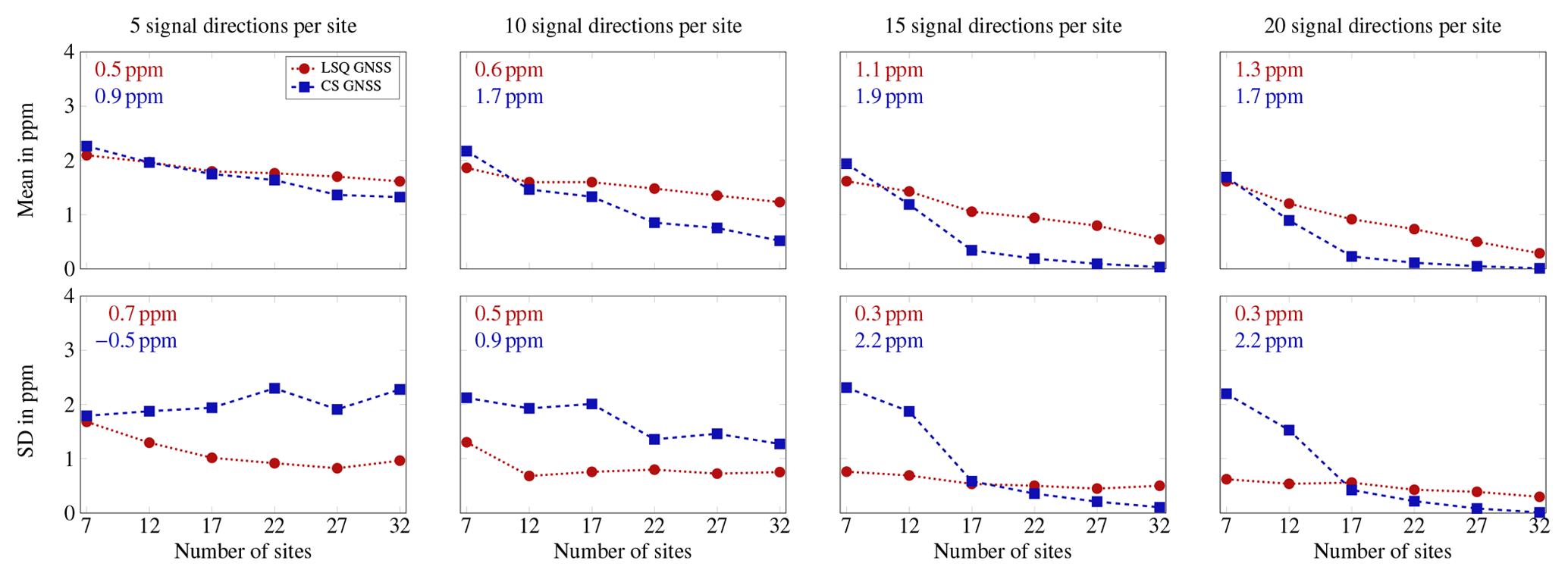
Figure 4Averaged over all voxels, this figure shows the mean of the absolute difference and the standard deviation (SD) of the difference between estimated refractivities and WRF refractivities in ppm, deduced from 48 samples of each investigated observing geometry setting composed of a certain number of synthetic GNSS sites and various numbers of signal directions per site. The dashed and dotted lines serve for better following the variation of the represented quantities with the number of sites, but only the discrete values indicated by the markers should be evaluated. The legend in the upper left subplot holds for all the subplots. In each subplot, the improvement by introducing 32 sites instead of 7 sites is given in red and blue. Degradations are given with a minus sign.
A more in-depth analysis does not show any significant differences among the individual voxels. Moreover, no significant systematics between the LSQ and CS solutions appeared, neither at the boundary layer nor at the top of the atmosphere. For most of the tested scenarios, LSQ provides better results than CS. However, if there are many sites and many different signal directions available, CS yields more accurate and more precise results than LSQ.
When investigating the standard deviation of the differences between estimated refractivities and WRF refractivities for the CS case, considering an increased number of synthetic GNSS sites only while keeping a constant number of five signal directions per site is not advantageous. However, as of 15 different signal directions per site, a clear improvement in standard deviation is visible when increasing the number of sites in the tomographic setting solved by means of CS. Independently of the number of sites, for realistic GPS-like observing geometry settings with 5 to 10 signal directions per site, the LSQ refractivity estimates are more precise than the CS refractivity estimates. In contrast, as of 15 signal directions per site, the CS solution yields more accurate and more precise refractivity estimates than the LSQ solution if at least 22 sites are available. That is, this study shows that LSQ is less sensitive to the number of signal directions than CS. Therefore, we recommend using LSQ for water vapor tomography with GPS-only observations and CS for water vapor tomography with multi-GNSS SWD estimates.
In the case of the maximum number of sites and the maximum number of signal directions per site (32 sites and 20 signal directions per site), when averaged over the 48 considered samples per observing geometry, the mean difference and the standard deviation of the LSQ or CS reconstruction attain values of about 0.3 ppm or 0.0 ppm. Therefore, the number of sites and the number of signal directions per site are of particular interest when aiming at a very accurate and very precise tomographic reconstruction using CS.
For the given voxel discretization with horizontal voxel sizes of 19 km and 20 km, the rule of thumb of Champollion et al. (2004) requires the mean intersite distance to correspond to no more than 19 to 20 km. The results show that, using the investigated synthetic data set with at least 15 signal directions per site, the CS solution is able to more accurately and more precisely reconstruct the atmospheric water vapor distribution than LSQ in the case of 22 sites within the 95×99 km2 large study area, i.e., at a site density of about 1 site per 20.7×20.7 km2, which is a bit lower than that required by the rule of thumb of Champollion et al. (2004). That is, if 15 signal directions are available per site, the rule of thumb can be transferred from the LSQ solution to water vapor tomography to CS solutions.
Consequently, the following three main results are summarized from this study.
-
The rule of thumb of Champollion et al. (2004) can be transferred from LSQ to CS.
-
Based on site distributions obeying the rule of thumb of Champollion et al. (2004), CS needs a variety of at least 15 signal directions per site in order to estimate the 3-D refractivity field more accurately and precisely than LSQ.
-
LSQ seems to be less sensitive to the number of signal directions than CS. Therefore, CS should only be used in the case of multi-GNSS SWD estimates yielding a variety of at least 15 signal directions per site.
Section 4 states not only that the rule of thumb of Champollion et al. (2004) holds for a tomographic solution based on LSQ, but also that it ensures a good tomographic reconstruction in the case of a CS solution. Although this finding is based on many different observing geometry settings, it only refers to a single voxel discretization and to a single study area with a single topography and a single site distribution within that study area. As a consequence, this research mainly investigates the validity of the rule of thumb of Champollion et al. (2004) for CS for the given study area, weather condition, and voxel discretization. For generalization, further tests should be performed that repeat the described methodology for other study areas, weather conditions, and voxel discretizations and for site distributions varying not only in the number but also the position of the sites. In particular, using only five vertical layers potentially represents limits to the validity of the results of the proposed approach.
Moreover, as the presented approach only relies on a synthetic data set deduced from WRF, the synthetic SWDs introduced within the tomographic system in this research are too optimistic when compared to real GNSS SWD estimates. Therefore, the conclusions drawn in Sect. 4 cannot necessarily be transferred to tomographic applications involving real SWD estimates. In order to get a better idea of the transferability of the results, the analysis should be repeated based on real data or the effect of adding different types of noise to the synthetic SWD estimates should be investigated (e.g., measurement and sensor noise and uncertainties resulting from the observing geometry). In the presented approach, instead of mapping ZWDs (zenith wet delays, related to SWDs by means of mapping as described, e.g., in Niell, 1996) to the slant signal directions as in the case of a real GNSS processing, the synthetic SWD data set is computed based on a direct ray tracing within the same voxels in which the tomographic reconstruction is thereafter performed. Yet, Heublein (2019) shows that this involves neglecting both a voxel discretization error and a mapping error committed in the case of real data.
Furthermore, Sect. 4 shows that the standard deviation of the difference between LSQ refractivity estimates and WRF refractivities is 6 % to 65 % smaller than that computed based on the CS refractivity estimates if at most 10 different signal directions per site are available. In contrast, in the case of a high number of sites and a high number of signal directions per site, the LSQ reconstruction is not able to yield as accurate and as precise estimates of the water vapor distribution as CS. That is, when solving the tomographic system by means of LSQ, increasing the number of SWD signal directions improves the tomographic reconstruction quality less than when using CS. This may be due to the geometric smoothing constraints forming the basis of the LSQ solution. In the case of a small number of observations, the smoothing constraints ensure a smooth solution free of outliers that does not necessarily correspond to the prevailing atmospheric conditions. In the case of a high variety of observations, the smoothing constraints become less important with respect to the data fidelity term within the LSQ solution to the tomographic system, but they still affect the tomographic solution. Even in the case of a very high number of observations, the tomographic system cannot be solved in a purely data-driven way. Instead, the tomographic solution always takes into account the chosen model assumptions; i.e., the LSQ solution always applies a certain amount of smoothing.
In addition, a low or high number of signal directions chosen from a synthetic multi-GNSS constellation for the recommendation of LSQ or CS for GPS-only or multi-GNSS water vapor tomography applications should not be set equal to considering a real GPS-only or real multi-GNSS setting. Choosing a small number of signal directions from a multi-GNSS constellation yields a higher variability in the signal directions than choosing the same small number of signal directions from a GPS-only constellation. Since a high number of signal directions proved to be of particular importance in the case of a CS solution, the quality of the refractivity estimates deduced using CS may decrease if real GPS-only signal directions are chosen.
Finally, future research should analyze in more detail which signal directions are necessary in an LSQ- or CS-based water vapor tomography in order to reconstruct well the refractivities of as many voxels as possible. A two-step CS LSQ may then first yield accurate refractivity estimates for most voxels by means of CS and then use the geometric smoothing constraints applied in LSQ to improve the refractivity estimates of those voxels in which CS yields inaccurate refractivity estimates even if a high number of sites and a high number of signal directions per site are available.
As the input data result from a cooperation and were exclusively provided for this research, they cannot be accessed online. For more information on the input data, please contact the Remote Sensing Technology Institute of the German Aerospace Center.
MH developed the theory and performed the computations. PEB and SH verified the analytical methods and supervised the findings of MH's work.
Within the last years, Marion Heublein and Stefan Hinz collaborated with the Signal Processing in Earth Observation (SiPEO) team of the German Aerospace Center and with former collaborators Giovanni Nico (Consiglio Nazionale delle Ricerche Bari, Italy) and Pedro Benevides (University of Lisbon, Portugal).
Thanks to Franz Ulmer (formerly at the German Aerospace Center at the Remote Sensing Technology Institute) for providing WRF data.
The first author was supported by a scholarship of the
Deutsche Telekom Stiftung. This publication of this research
has been supported by the KIT-Publication Fund of the
Karlsruhe Institute of Technology (grant application no. 1189).
The article processing charges for this open-access
publication were covered by a Research
Centre of the Helmholtz Association.
This paper was edited by Gunter Stober and reviewed by two anonymous referees.
Aguilera, E., Nannini, M., and Reigber, A.: A data-adaptive compressed sensing approach to polarimetric SAR tomography of forested areas, IEEE Geosci. Remote Sens. Lett., 10, 543–547, 2013. a
Alonso, M. T., López-Dekker, P., and Mallorquí, J. J.: A novel strategy for radar imaging based on compressive sensing, IEEE T. Geosci. Remote Sens., 48, 4285–4295, 2010. a
Baraniuk, R.: Compressive sensing, IEEE Signal Proc. Mag., 24, 118–120, 2007. a
Bender, M. and Raabe, A.: Preconditions to ground based GPS water vapour tomography, Ann. Geophys., 25, 1727–1734, https://doi.org/10.5194/angeo-25-1727-2007, 2007. a
Bender, M., Dick, G., Wickert, J., Ramatschi, M., Ge, M., Gendt, G., Rothacher, M., Raabe, A., and Tetzlaff, G.: Estimates of the information provided by GPS slant data observed in Germany regarding tomographic applications, J. Geophys. Res.-Atmos., 114, D06303, https://doi.org/10.1029/2008JD011008, 2009. a
Bender, M., Dick, G., Ge, M., Deng, Z., Wickert, J., Kahle, H.-G., Raabe, A., and Tetzlaff, G.: Development of a GNSS water vapour tomography system using algebraic reconstruction techniques, Adv. Space Res., 47, 1704–1720, https://doi.org/10.1016/j.asr.2010.05.034, 2011a. a
Bender, M., Stosius, R., Zus, F., Dick, G., Wickert, J., and Raabe, A.: GNSS water vapour tomography–Expected improvements by combining GPS, GLONASS and Galileo observations, Adv. Space Res., 47, 886–897, 2011b. a
Budillon, A., Evangelista, A., and Schirinzi, G.: Three-dimensional SAR focusing from multipass signals using compressive sampling, IEEE T. Geosci. Remote Sens., 49, 488–499, 2011. a
Candès, E. J. and Wakin, M. B.: An introduction to compressive sampling, IEEE Signal Proc. Mag., 25, 21–30, 2008. a
Candès, E. J.: Compressive sampling, in: Proceedings of the international congress of mathematicians, Vol. 3, 1433–1452, European Mathematical Society Publishing House, Madrid, Spain, 2006. a, b
Champollion, C., Masson, F., Bouin, M.-N., Walpersdorf, A., Doerflinger, E., Bock, O., and Van Baelen, J.: GPS water vapour tomography: preliminary results from the ESCOMPTE field experiment, Atmos. Res., 74, 253–274, 2004. a, b, c, d, e, f, g, h, i, j, k, l
Davis, J. L., Elgered, G., Niell, A. E., and Kuehn, C. E.: Ground-based measurement of gradients in the “wet” radio refractivity of air, Radio Sci., 28, 1003–1018, 1993. a
Ding, N., Zhang, S., Wu, S., Wang, X., Kealy, A., and Zhang, K.: A new approach for GNSS tomography from a few GNSS stations, Atmos. Meas. Tech., 11, 3511–3522, https://doi.org/10.5194/amt-11-3511-2018, 2018. a
Donoho, D. L.: Compressed sensing, IEEE T. Inform. Theory, 52, 1289–1306, 2006. a
Elosegui, P., Ruis, A., Davis, J., Ruffini, G., Keihm, S., Bürki, B., and Kruse, L.: An experiment for estimation of the spatial and temporal variations of water vapor using GPS data, Phys. Chem. Earth, 23, 125–130, https://doi.org/10.1016/S0079-1946(97)00254-1, 1998. a
Feairheller, S. and Clark, R.: Other satellite navigation systems, Understanding GPS–principles and applications, 2nd Edn., Artech House, Norwood, 595–634, 2006. a
Flores, A., Ruffini, G., and Rius, A.: 4D tropospheric tomography using GPS slant wet delays, Ann. Geophys., 18, 223–234, https://doi.org/10.1007/s00585-000-0223-7, 2000. a, b, c, d
Gradinarsky, L. P. and Jarlemark, P.: Ground-based GPS tomography of water vapor: Analysis of simulated and real data, J. Meteorol. Soc. Jpn., 82, 551–560, 2004. a, b
Grohnfeldt, C., Zhu, X. X., and Bamler, R.: Jointly sparse fusion of hyperspectral and multispectral imagery, in: IEEE Geoscience and Remote Sensing Symposium (IGARSS), 4090–4093, 2013 IEEE International, Melbourne, VIC, Australia, 2013. a
Hansen, M. H. and Yu, B.: Model selection and the principle of minimum description length, J. Am. Stat. Assoc., 96, 746–774, 2001. a
Heublein, M.: GNSS and InSAR based water vapor tomography: A Compressive Sensing solution, PhD thesis, Karlsruhe Institute of Technology (KIT), https://doi.org/10.5445/IR/1000093403, 2019. a, b, c, d, e, f, g, h, i, j, k
Heublein, M., Alshawaf, F., Erdnüß, B., Zhu, X. X., and Hinz, S.: Compressive sensing reconstruction of 3D wet refractivity based on GNSS and InSAR observations, J. Geodesy, 93, 197–217, https://doi.org/10.1007/s00190-018-1152-0, 2018. a, b, c, d, e, f, g, h, i, j
Hirahara, K.: Local GPS tropospheric tomography, Earth Planets Space, 52, 935–939, https://doi.org/10.1186/BF03352308, 2000. a, b
Hofmann-Wellenhof, B., Lichtenegger, H., and Wasle, E.: GNSS – Global Navigation Satellite Systems: GPS, GLONASS, Galileo and more, Springer, Wien, https://doi.org/10.1007/978-3-211-73017-1, 2008. a
Hurter, F. and Maier, O.: Tropospheric profiles of wet refractivity and humidity from the combination of remote sensing data sets and measurements on the ground, Atmos. Meas. Tech., 6, 3083–3098, https://doi.org/10.5194/amt-6-3083-2013, 2013. a
Jiang, C., Zhang, H., Shen, H., and Zhang, L.: Two-step sparse coding for the pan-sharpening of remote sensing images, IEEE J. Sel. Top. Appl., 7, 1792–1805, 2014. a
Li, S. and Yang, B.: A new pan-sharpening method using a compressed sensing technique, IEEE T. Geosci. Remote Sens., 49, 738–746, 2011. a
Niell, A.: Global mapping functions for the atmosphere delay at radio wavelengths, J. Geophys. Res.-Sol. Ea., 101, 3227–3246, 1996. a
Nilsson, T. and Elgered, G.: Water vapour tomography using GPS phase observations: Results from the ESCOMPTE experiment, Tellus A, 59, 674–682, 2007. a
Notarpietro, R., Gabella, M., and Perona, G.: Tomographic reconstruction of neutral atmospheres using slant and horizontal wet delays achievable through the processing of signal observed from small GPS networks, Ital. J. Remote Sens., 40, 63–74, 2008. a
Perler, D.: Water vapor tomography using global navigation satellite systems, PhD thesis, Diss., Eidgenössische Technische Hochschule ETH Zürich, No. 20012, 2011. a
Potter, L. C., Ertin, E., Parker, J. T., and Cetin, M.: Sparsity and compressed sensing in radar imaging, P. IEEE, 98, 1006–1020, 2010. a
Pruente, L.: Application of compressed sensing to SAR/GMTI-data, in: Synthetic Aperture Radar (EUSAR), 2010 8th European Conference on, 1–4, VDE, Aachen, Germany, 2010. a
Rauhut, H.: Compressive sensing and structured random matrices, in: Theoretical foundations and numerical methods for sparse recovery, 9, 1–92, Walter de Gruyter https://doi.org/10.1515/9783110226157.1, 2010. a
Rohm, W.: The precision of humidity in {GNSS} tomography, Atmos. Res., 107, 69–75, https://doi.org/10.1016/j.atmosres.2011.12.008, 2012. a, b
Rohm, W.: The ground GNSS tomography–unconstrained approach, Adv. Space Res., 51, 501–513, 2013. a
Rohm, W., Zhang, K., and Bosy, J.: Limited constraint, robust Kalman filtering for GNSS troposphere tomography, Atmos. Meas. Tech., 7, 1475–1486, https://doi.org/10.5194/amt-7-1475-2014, 2014. a
Skamarock, W. C., Klemp, J. B., Dudhia, J., Gill, D. O., Barker, D. M., Wang, W., and Powers, J. G.: A description of the advanced research WRF version 2, Tech. rep., National Center For Atmospheric Research Boulder Co Mesoscale and Microscale Meteorology Div, Tech. Note TN-475+STR, https://doi.org/10.5065/D6DZ069T, 2005. a
Song, S., Zhu, W., Ding, J., and Peng, J.: 3D water-vapor tomography with Shanghai GPS network to improve forecasted moisture field, Chinese Sci. Bull., 51, 607–614, https://doi.org/10.1007/s11434-006-0607-5, 2006. a
Troller, M.: GPS based determination of the integrated and spatially distributed water vapor in the troposphere, Vol. 67, ETH Zurich, Zurich, 2004. a
Xia, P., Cai, C., and Liu, Z.: GNSS troposphere tomography based on two-step reconstructions using GPS observations and COSMIC profiles, Ann. Geophys., 31, 1805–1815, https://doi.org/10.5194/angeo-31-1805-2013, 2013. a
Zhao, Q., Yao, Y., Cao, X., and Yao, W.: Accuracy and reliability of tropospheric wet refractivity tomography with GPS, BDS, and GLONASS observations, Adv. Space Res., 63, 2836–2847, 2019. a
Zhu, X. X. and Bamler, R.: Tomographic SAR inversion by L1-norm regularization – The compressive sensing approach, IEEE T. Geosci. Remote Sens., 48, 3839–3846, 2010. a
Zhu, X. X. and Bamler, R.: A sparse image fusion algorithm with application to pan-sharpening, IEEE T. Geosci. Remote Sens., 51, 2827–2836, 2013. a
Zhu, X. X. and Bamler, R.: Superresolving SAR tomography for multidimensional imaging of urban areas: Compressive sensing-based TomoSAR inversion, IEEE Signal Proc. Mag., 31, 51–58, 2014. a
Zhu, X. X., Grohnfeldt, C., and Bamler, R.: Exploiting joint sparsity for pansharpening: The J-SparseFI algorithm, IEEE T. Geosci. Remote Sens., 54, 2664–2681, 2016. a