Odd hydrogen response thresholds for indication of solar proton and electron impact in the mesosphere and stratosphere

Understanding the atmospheric forcing from energetic particle precipitation (EPP) is important for climate simulations on decadal time scales. However, presently there are large uncertainties in energy flux measurements of electron precipitation. One approach to narrowing these uncertainties is by analyses of EPP direct atmospheric impacts and their relation to measured EPP fluxes. Here we use observations from the microwave limb sounder (MLS) and Whole Atmosphere Community Climate Model (WACCM) simulations, together with EPP fluxes from the Geostationary Operational Environmental Satellite (GOES) and Polar-orbiting Operational Environmental Satellite (POES) to determine the OH and HO₂ response thresholds to solar proton events (SPEs) and radiation belt electron (RBE) precipitation. Because of their better signal-to-noise ratio and extended altitude range, we utilize MLS HO₂ data from an improved offline processing instead of the standard operational product. We consider a range of altitudes in the middle atmosphere and all magnetic latitudes from pole to pole. We find that the nighttime flux limits for day-to-day EPP impact detection using OH and HO₂ are 50–130 $\mathrm{protons}{\mathrm{cm}}^{-\mathrm{2}}{\mathrm{s}}^{-\mathrm{1}}{\mathrm{sr}}^{-\mathrm{1}}$ (E>10 MeV) and 1.0–2.5×10⁴ $\mathrm{electrons}{\mathrm{cm}}^{-\mathrm{2}}{\mathrm{s}}^{-\mathrm{1}}{\mathrm{sr}}^{-\mathrm{1}}$ (E = 100–300 keV). Based on the WACCM simulations, nighttime OH and HO₂ are good EPP indicators in the polar regions and provide best coverage in altitude and latitude. Due to larger background concentrations, daytime detection requires larger EPP fluxes and is possible in the mesosphere only. SPE detection is easier than RBE detection because a wider range of polar latitudes is affected, i.e., the SPE impact is rather uniform poleward of 60^∘, while the RBE impact is focused at 60^∘. Altitude-wise, the SPE and RBE detection are possible at ≈ 35–80 and ≈ 65–75 km, respectively. We also find that the MLS OH observations indicate a clear nighttime response to SPE and RBE in the mesosphere, similar to the simulations. However, the MLS OH data are too noisy for response detection in the stratosphere below 50 km, and the HO₂ measurements are overall too noisy for confident EPP detection on a day-to-day basis.

1 Introduction

Solar energetic particle precipitation (EPP) affects the polar atmospheric chemistry directly at the altitude region from the upper stratosphere to the lower thermosphere. Ionization caused by precipitating protons and electrons leads to, for example, the production of odd hydrogen and odd nitrogen from ionic reactions and, subsequently, to the loss of ozone through catalytic reactions (Sinnhuber et al., 2012). There is evidence of EPP-driven variability in winter–springtime ozone (Andersson et al., 2014a; Damiani et al., 2016), which could further connect to decadal variability in regional climate via modulation of polar vortex dynamics and the top-down coupling (e.g., Seppälä et al., 2014).

In atmospheric and climate modeling, EPP forcing can be defined using satellite-based particle flux observations (Matthes et al., 2017, and references therein). Solar wind proton fluxes are continuously measured by detectors aboard the Geostationary Operational Environmental Satellites (GOES) in the geosynchronous orbit (https://www.ngdc.noaa.gov/stp/satellite/goes/, last access: 17 December 2020). These measurements provide a good representation of proton forcing because MeV protons have enough rigidity, i.e., momentum/charge, to penetrate through Earth's magnetic field in polar regions and enter the atmosphere directly from the solar wind. Several studies have shown that the observed atmospheric effects can be well represented in models using the GOES proton observations if the relevant ion-neutral chemistry is considered as well (Jackman et al., 2001; Verronen et al., 2006; Funke et al., 2011; Andersson et al., 2016). For electron precipitation, the situation is different. Electrons have less mass than protons and are captured by Earth's magnetosphere, e.g., in the radiation belts (Baker et al., 2018), from where they are eventually lost either to space or into the atmosphere. Satellite-based observations of electron precipitation fluxes are being made from low-orbiting satellites, but these measurements do not capture full spatiotemporal variability and also suffer from restricted measurement geometry and proton contamination, like in the case of the Medium Energy Proton And Electron Detector (MEPED) and Polar-orbiting Operational Environmental Satellite (POES) instruments (Rodger et al., 2010a; van de Kamp et al., 2018). Atmospheric impacts seen in observations seem to indicate a need for a large adjustment of the electron-forcing representation in simulations (Clilverd et al., 2012; Randall et al., 2015). Thus atmospheric observations of EPP impact could help in understanding the uncertainties in the electron flux data and how these flux observations relate to effects in the atmosphere (e.g. Verronen et al., 2011). Thus, EPP detection limits for atmospheric data are valuable information.

Ground-based ionospheric observations provide the most direct measure of EPP atmospheric impact (e.g., Verronen et al., 2015; Heino et al., 2019), but in practice, only satellite-based measurements can offer a global view. Measurement of odd hydrogen species (OH and HO₂) are well suited for monitoring EPP impacts due to their relative short chemical lifetime (Verronen et al., 2006; Damiani et al., 2010a). Satellite-based observations of OH were made continuously in 2004–2009 by the microwave limb sounder (MLS) aboard the Aura satellite (Pickett et al., 2006a, b, 2008). They have since been used to study both solar proton events and electron precipitation (Verronen et al., 2006; Damiani et al., 2010a; Jackman et al., 2011; Andersson et al., 2012; Verronen et al., 2013; Jackman et al., 2014; Andersson et al., 2014b), particularly at 60–80 km altitudes where the largest EPP events can produce order-of-magnitude increases. Compared to the OH observations, MLS HO₂ measurements have been made since 2004 and, thus, provide a longer time series than the OH observations. However, the standard HO₂ data from operational processing have a lower signal-to-noise ratio and only cover the lower mesosphere and stratosphere (Pickett et al., 2008; Livesey et al., 2018). Thus, the use of standard HO₂ data has been limited to large proton events (Jackman et al., 2011; Zou et al., 2018). An improved offline processing of HO₂ data provides better quality (Millán et al., 2015), extending the altitude range to the mesopause and enhancing possibilities for studies of daily EPP impact.

In this paper, we use MLS observations of OH and HO₂ to determine EPP flux thresholds for impact detection in the stratosphere and mesosphere. Looking at different latitude bands and altitudes individually, we first consider large proton events, which have a well-known flux from satellite observations, to develop a method for EPP threshold detection. We then apply the same method to medium-energy electrons for which the satellite-based flux observations are not all inclusive. We compare satellite-data-based thresholds to those from the Whole Atmosphere Community Climate Model (WACCM, version 4) to discuss both limitations of the satellite data and EPP forcing in WACCM. Our results provide the limits of MLS OH and HO₂ for EPP detection and usability in EPP studies.

2 Data and models

The microwave limb sounder (MLS) measures millimeter and submillimeter thermal emissions from the Earth's limb atmosphere from which temperature, trace gases, and cloud ice are retrieved. Launched in July 2004 into a Sun-synchronous near-polar orbit, the geographic latitude coverage of the measurements is from 82^∘ S to 82^∘ N on each orbit, and measurements are made during both day and night conditions. The instrument is described in detail by Waters et al. (2006). A detailed description of MLS version 4 data products and quality is given by Livesey et al. (2018). The MLS target species in the stratosphere and mesosphere include OH and HO₂.

For the version 4 OH data used in our study, the recommended pressure range of observations is 32–0.0032 hPa (approx. altitudes 25–95 km). At levels with p>0.01 hPa, the vertical resolution of observations is 2.5 km. Version 2.2 data have been validated with balloon-borne remote sensing instruments and with ground-based column measurements (Pickett et al., 2008; Wang et al., 2008). Instead of the standard HO₂ data, we use data from the offline processing described in detail and validated against other observations by Millán et al. (2015). This algorithm retrieves daily zonal means of HO₂ over an extended vertical range by first averaging the radiances in 10^∘ bins, resulting in a better signal-to-noise ratio and an extended altitude range compared to the standard HO₂ data. The recommended pressure range for the offline HO₂ data is 10–0.0032 hPa (≈ 35–90 km), and the vertical resolution is about 4 km between 10 and 0.1 hPa, 8 km at 0.02 hPa, and around 14 km for lower pressures. Daytime and nighttime data are provided separately, using measurement tangent point solar zenith angle limits <90 and $>{\mathrm{100}}^{\circ }$, respectively.

The Whole Atmosphere Community Climate Model (WACCM) is a chemistry–climate model that extends from the surface to about $\mathrm{5.9}\times {\mathrm{10}}^{-\mathrm{6}}$ hPa (≈140 km), with a horizontal resolution of 1.9^∘ latitude by 2.5^∘ longitude. WACCM physics and atmospheric responses to solar and geomagnetic forcing variations are described by Marsh et al. (2007). Details about WACCM version 4 coupled simulations and an overview of the model climate can be found in Marsh et al. (2013). Here, we utilize WACCM-D, a variant of WACCM version 4 in which standard parameterization of EPP-driven odd hydrogen and odd nitrogen production is replaced by a set of D-region ion chemistry reactions (Verronen et al., 2016) and which better reproduces the observed OH response during EPP (Andersson et al., 2016). We used WACCM-D in the specified dynamics scenario (SD-WACCM-D) forced with meteorological fields (temperature, winds, and surface pressure) from the Modern-Era Retrospective analysis for Research and Applications (MERRA; Rienecker et al., 2011). The daily atmospheric ionization rates due to 1–300 MeV solar protons are calculated based on flux data available from the National Oceanic and Atmospheric Administration (NOAA) Space Environment Center (https://www.ngdc.noaa.gov/stp/satellite/goes/dataaccess.html, last access: 17 December 2020) and the methodology discussed in Jackman et al. (2009). These are applied at geomagnetic latitudes $>{\mathrm{60}}^{\circ }$ in both hemispheres. The daily zonal mean ionization rates at geomagnetic latitudes 40–72^∘ from precipitating 30–1000 keV electrons are taken from the APEEP (Ap-driven energetic electron precipitation) proxy model, which is recommended for the Coupled Model Intercomparison Project (CMIP; van de Kamp et al., 2016; Matthes et al., 2017). We carried out a simulation for a period between 2000–2012, which covers the whole period of MLS OH observations. WACCM-D output, including OH and HO₂, was saved at MLS measurement times and locations to ensure a one-to-one match between the model and the measurements in the analysis.

EPP forcing patterns follow the geomagnetic latitudes rather than the geographic ones, and the odd hydrogen response is expected to show similar patterns due to its short chemical lifetime (e.g., Andersson et al., 2018). Thus, we use a modified version of the HO₂ offline algorithm in which the radiances were averaged using geomagnetic latitudes instead of geographic latitudes (for a definition of altitude-adjusted corrected geomagnetic coordinates, see, e.g., Shepherd, 2014). These geomagnetic latitudes are shown in Fig. 1. Before the analysis, the MLS OH and WACCM-D data were preprocessed the same way as it was done for HO₂. The data were divided into daily daytime and nighttime sets, using the same solar zenith angle limits, and averaged zonally after sorting observations into 10^∘ geomagnetic latitude bins, running from $-{\mathrm{85}}^{\circ }$ through to $+{\mathrm{85}}^{\circ }$. Through this paper, these bins are referred to by their central latitude, i.e., the latitude 40^∘ refers to the zonal average from geomagnetic latitudes 35–45^∘. It should be noted that, due to separating the data both by latitude and by day/night conditions, there is sometimes little data available at the highest latitudes. For example, sometimes there is no nighttime data in June for latitude 80^∘. The daily averages of existing data points at the high geomagnetic latitude bins may also be skewed towards lower geographic latitudes. However, this should not affect our comparisons because WACCM-D was sampled at the MLS times and locations and binned in the same manner.

Figure 1 Geomagnetic latitude bin limits used in the analysis.

In the analysis, we use the pressure level grid from the MLS measurements, as sections of the MLS HO₂ and OH pressure grids are the same. Hence, the overlapping sections of MLS HO₂ and OH values were selected, whereas the least squares interpolation method recommended by Livesey et al. (2018) was used to convert WACCM-D data onto the MLS grid. The same pressure grid allows for direct comparisons between the data sets. The MLS HO₂ offline data are provided in both mixing ratios (parts per million by volume – ppmv) and concentrations ($\mathrm{molec}.{\mathrm{cm}}^{-\mathrm{3}}$). Thus, daily total density profiles can be calculated by dividing HO₂ concentrations by HO₂ mixing ratios. To ensure consistency between the data sets, MLS OH and WACCM-D data were converted from mixing ratios to concentrations using the same total densities from MLS HO₂. For the general comparisons, the MLS HO₂ averaging kernels were applied to the WACCM-D HO₂ fields. As most of the averaging kernels are fairly similar, only the daytime and nighttime kernels corresponding to magnetic equator were used and applied to all latitude bins. MLS averaging kernels were not used on WACCM-D OH data because the effect was expected to be small. In the threshold detection, the MLS averaging kernels were not applied on WACCM-D HO_x data.

In order to show the connection between EPP and odd hydrogen changes, we use proton flux measurements from the Geostationary Operational Environmental Satellite (GOES-11; https://www.ngdc.noaa.gov/stp/satellite/goes/, last access: 17 December 2020) as a measure of proton precipitation over the polar caps. Daily average fluxes of protons with energies greater than 10 MeV are used as an indicator because those directly affect atmospheric altitudes below about 90 km (for the relation between EPP energies and penetration altitudes, see Turunen et al., 2009, Fig. 3). The measurements from the other GOES channels responding to higher proton energies correlate well with the >10 MeV channel (not shown), so we would not expect significant changes in our results if other proton energy channels were used. As a measure of electron precipitation, we use flux observations from the Medium Electron Proton and Electron Detector (MEPED) aboard the Polar Orbiting Environmental Satellite (POES; Evans and Greer, 2004). Daily average electron fluxes from an energy range between 100 and 300 keV, and from the 50^∘ magnetic latitude bin, are used as indicator of the radiation belt electron precipitation (RBE) affecting mesospheric altitudes. While the magnitude of RBE forcing will depend on latitude more than for the proton forcing, the 50^∘ latitude bin was selected because of its most pronounced atmospheric HO_x impact (e.g., Verronen et al., 2011). The assumption here is that the RBE forcing will vary similarly with magnetic activity across affected latitudes, although the magnitude can differ. The electron flux data are exclusively from the zero-degree telescope and have been preprocessed to remove known quality issues (for a description, see Verronen et al., 2011, and references therein), e.g., data suffering from proton contamination have been excluded using the methods described by Rodger et al. (2010a).

3 Methods

First, we present an overall comparison between WACCM-D and MLS odd hydrogen data. We use monthly average concentrations to identify the main similarities and differences between the data sets, focusing on the shape, strength, and location of concentration peaks. These comparisons provide us with information on the overall representation of odd hydrogen in WACCM-D, which can help us to understand the differences in EPP detection thresholds.

Starting from the approach of Verronen et al. (2011), we use daily average data in EPP detection. However, Verronen et al. (2011) studied only four selected RBE events, and although they demonstrated the correlation between EPP and OH, they did not use HO₂ data or pursue the detection limits. Before determining threshold values for the SPE and RBE detection, daily climatologies of OH and HO₂ concentrations were removed from the odd hydrogen data. Climatological values were calculated for each day of the year by first calculating the daily average OH and HO₂ night and day concentrations of available data at each grid point, separately, for WACCM-D and MLS. A 9 d moving average was then calculated to smooth the time series and produce the final climatologies. After the climatology is removed, the background concentrations do not display seasonal variability, which makes it possible to combine EPP event periods from different seasons for the threshold detection. Examples of this deseasonalizing effect can be seen in Fig. 2.

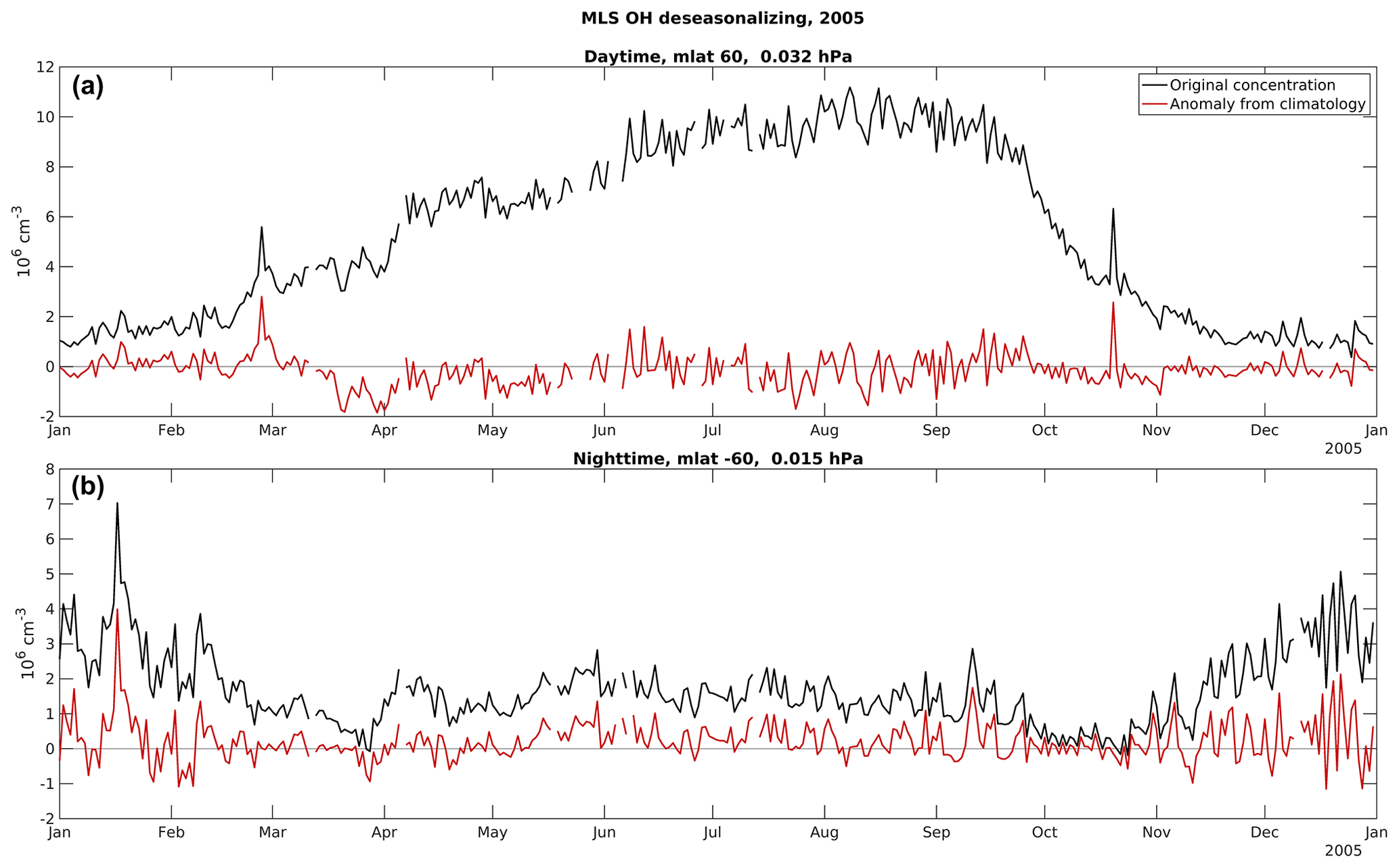
Figure 2 Daily MLS OH concentrations (in black) and the deseasonalized anomalies from the climatology (red) in 2005. Daytime (a) on magnetic latitude 60^∘ N at 0.032 hPa and nighttime (b) on magnetic latitude 60^∘ S at 0.015 hPa.

It should be noted that after the climatology is removed, the HO_x concentrations still have variability from sources other than EPP, and these are included in the data in our analysis. For example, sudden stratospheric warmings (SSWs) contribute to the year-to-year OH variability in the Northern Hemisphere (NH) middle atmosphere (Damiani et al., 2010b). As our aim is to determine the general threshold values for SPE and RBE detection, we do not separate SSWs years in any particular manner. However, we consider Southern Hemisphere (SH) and NH separately, and only the NH is regularly affected by SSWs.

For the SPE threshold determination, we selected data from all months during which the daily proton flux indicates an event, i.e., it exceeds the limit of 10 $\mathrm{protons}{\mathrm{cm}}^{-\mathrm{2}}{\mathrm{s}}^{-\mathrm{1}}{\mathrm{sr}}^{-\mathrm{1}}$ (see Fig. 3a). All months used in the analysis are listed in Table 1. Using data from the selected months, we applied a fitting method previously used by Verronen et al. (2011). First, we plotted the SPE flux values against the climatology-free odd hydrogen concentrations (i.e., anomalies). Then, a first-degree polynomial was fitted to the HO_x anomalies and the square root of the SPE fluxes. A limit for a significant SPE-driven enhancement in odd hydrogen concentration was calculated by adding the standard deviation of the concentrations to the median concentration. Since the concentrations are deseasonalized, the median is expected to be close to zero. The addition of the standard deviation suggests that a concentration anomaly of 1 standard deviation from the climatology is significant and should be detected. We then find the SPE indicator value at the intersection of the limit and the linear fit; this is the detected SPE threshold flux value. Examples of the SPE threshold determination are shown in Fig. 4a. This process is applied for each latitude bin and at each pressure level separately. To identify those thresholds that are reasonable, they are filtered using correlations between the square root of the SPE fluxes and odd hydrogen concentrations. All thresholds with corresponding correlation coefficient ≥0.35 are accepted as reasonable, and the rest are discarded. This filtering effectively removes threshold values at lower latitudes where SPE impact is not expected.

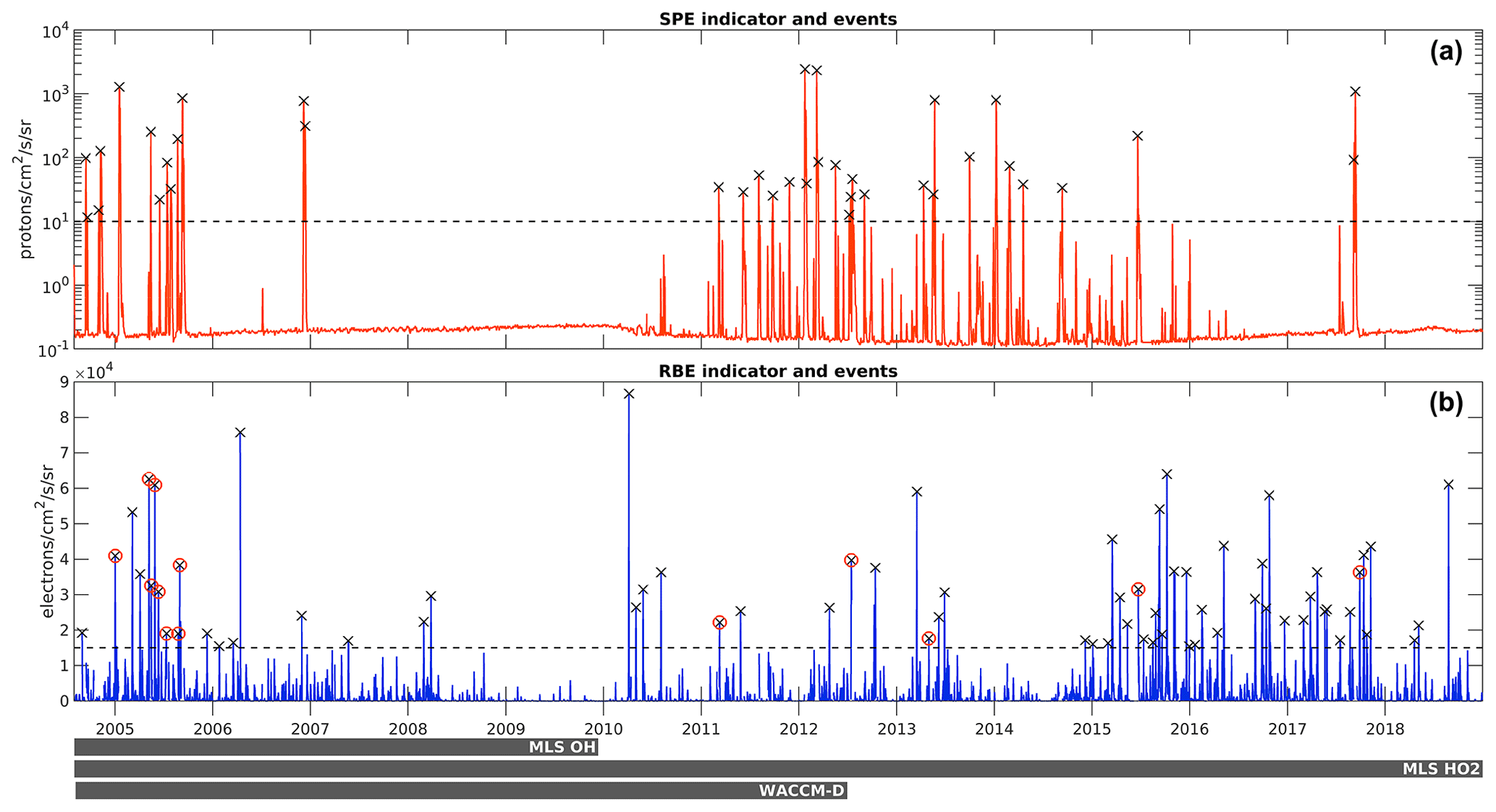
Figure 3 SPE indicator (a) and RBE indicator (b). Used precipitation limits for events are shown as dashed lines, and precipitation events are indicated by crosses. Encircled crosses mark RBE events with an SPE event in the same month. Availability of MLS OH and HO₂ and WACCM-D data used in the analysis is also shown below the graphs.

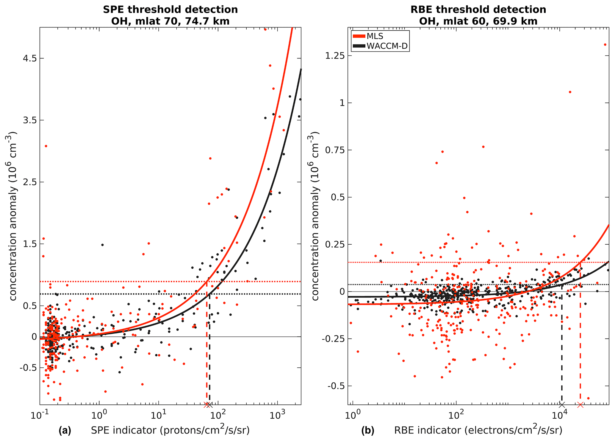
Figure 4 Precipitation threshold determination using nighttime OH. (a) SPE indicator at magnetic latitude 70^∘ N and 0.0215 hPa (74.7 km) and (b) RBE indicator at magnetic latitude 60^∘ N and 0.0464 hPa (69.9 km). MLS data in red and WACCM-D in black. Daily indicator and OH concentration value pairs are shown as dots, and the linear fit is shown as a solid line. Used limits (median and SD; dotted horizontal lines) and detected threshold values (dashed vertical lines) are also shown. Note that the linear fitting was done using the square roots of the flux indicator values.

Table 1 Months included in the analysis, with dates (dd.mm.yyyy) of SPE and RBE flux peaks within each month (month/year) also given. For peaks within 5 d of each other, only the date of the strongest is included. Dates marked by ^a indicate dates in months where the event peak was in another month. RBE peak dates marked by ^b are not included in the analysis, due to an SPE peak in the same month.

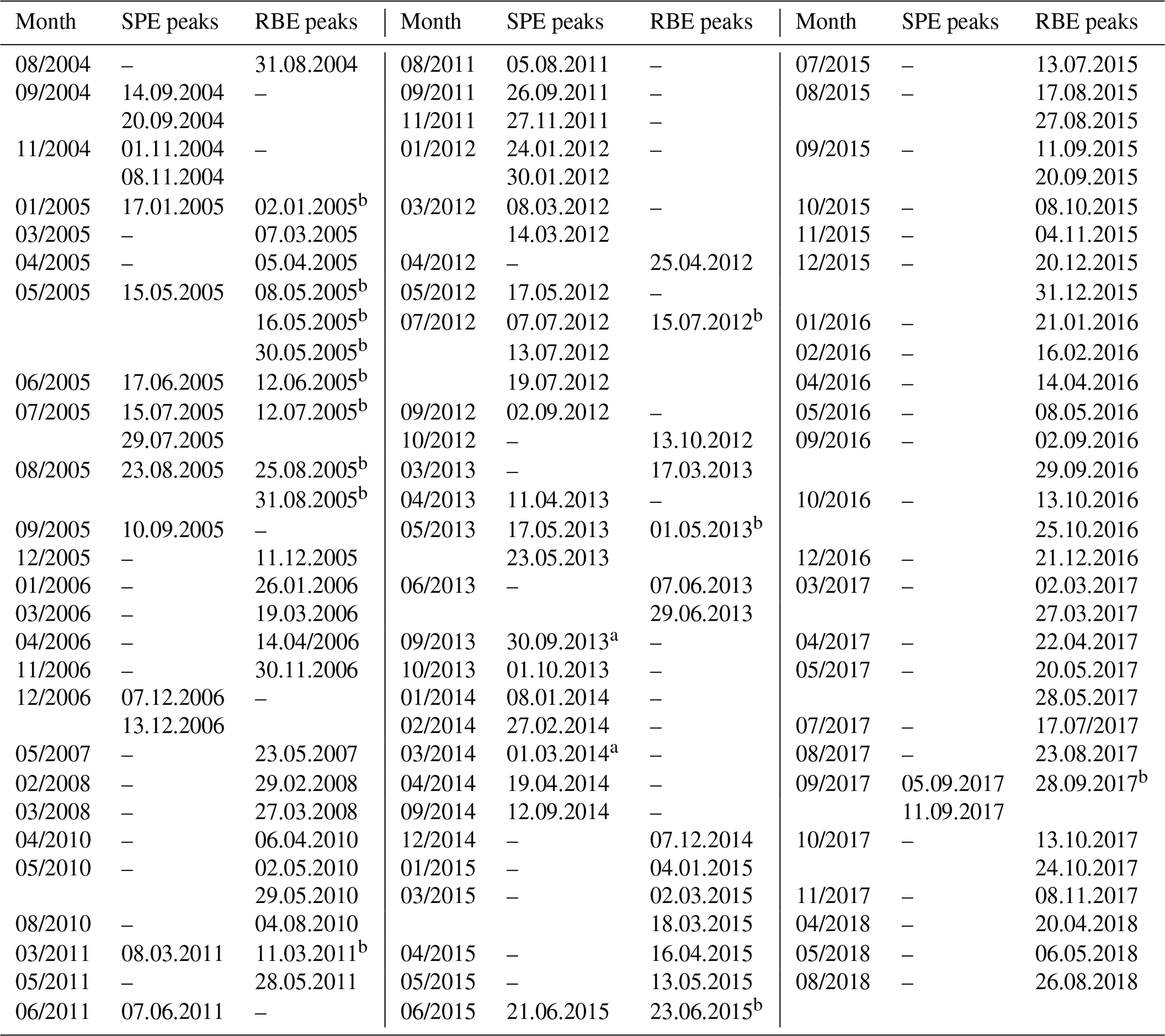
The RBE threshold values are determined using the same method but with different RBE flux and correlation limits. RBE months were found using an RBE flux limit of 1.5×10⁴ $\mathrm{electrons}{\mathrm{cm}}^{-\mathrm{2}}{\mathrm{s}}^{-\mathrm{1}}{\mathrm{sr}}^{-\mathrm{1}}$ (see Fig. 3b), and data from these months are used in the analysis. However, the months with an SPE event, as defined in the previous paragraph, were excluded. The RBE fluxes from MEPED are not reliable during SPEs (Rodger et al., 2010a), and SPE forcing would likely interfere with the RBE threshold detection. Indeed, exclusion of SPE months leads to stronger correlations between the RBE flux and odd hydrogen concentrations (not shown). For a full list of the months used in the analysis, refer to Table 1. As with SPEs, the RBE thresholds were found using linear fitting with square roots and the median and the standard deviation of odd hydrogen data (see Fig. 4b). For RBE events, threshold values with corresponding flux–concentration correlation coefficients ≥0.25 are accepted as reasonable.

As seen in Fig. 4a at 0.1–0.2 $\mathrm{protons}{\mathrm{cm}}^{-\mathrm{2}}{\mathrm{s}}^{-\mathrm{1}}{\mathrm{sr}}^{-\mathrm{1}}$, in some cases there is a large number of data points at low fluxes. To find out the impact on our analysis, we performed tests where we excluded these low-flux points. In general, correlations between flux data and HO_x concentrations become stronger, but thresholds increase due to larger standard deviation. These effects would, however, not change our conclusions.

4 Results

4.1 Overall comparison between WACCM-D and MLS

In general, WACCM-D and MLS compare reasonably well in the magnitude and spatiotemporal variability in OH and HO₂. In both MLS and WACCM-D daytime concentration profiles, there is a maximum in the stratosphere and mesosphere, which reflects the production being dependent on atomic oxygen and Lyman-alpha radiation, respectively. Figure 5 shows a time series of monthly average daytime concentrations at magnetic latitude 70^∘ N, and these peaks and the seasonality of HO_x concentrations are clear in both MLS and WACCM-D. Overall, the greatest concentrations are seen in the summer months. Latitude-wise, the strongest concentrations are found at lower latitudes, with concentrations generally decreasing polewards (not shown). Lower latitudes also show the clearest stratospheric and mesospheric maxima and less seasonal variability than the polar regions.

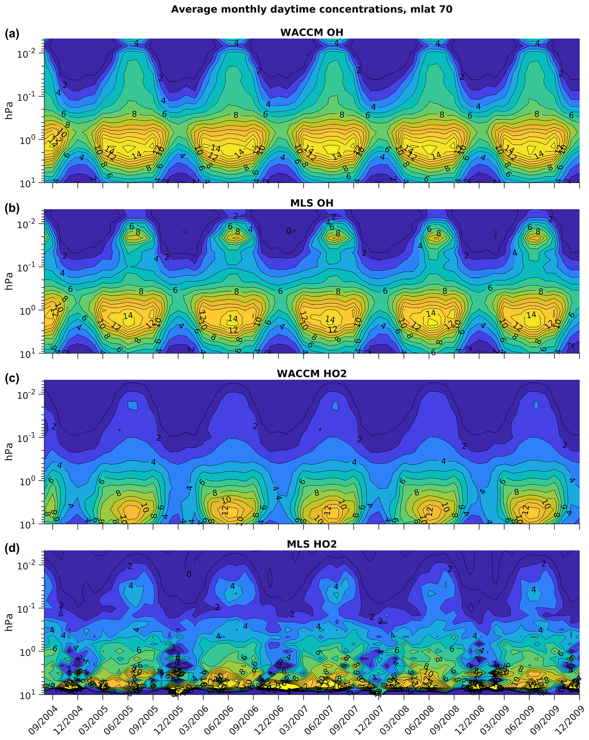
Figure 5 Monthly average daytime OH and HO₂ concentrations on magnetic latitude 70^∘ N. From (a) to (d): WACCM-D OH; MLS OH; WACCM-D HO₂; MLS HO₂. Concentrations are in units 10⁶ cm⁻³.

WACCM-D shows a stronger stratospheric OH peak by 10 %–20 % and a weaker mesospheric OH peak by up to a factor of 2. In WACCM-D, the vertical transition between the OH summertime peaks is more continuous, while in MLS data there is a clear minimum between them around 0.1 hPa. EPP detection in the summer mesosphere is likely harder from MLS than WACCM-D because of larger background concentrations. In wintertime, both WACCM-D and MLS show lower OH values than in summer, particularly in the mesospheric altitudes, while the altitude distributions and concentrations are very similar. Similar observations can be made in daytime HO₂ data as well (Fig. 5). Of the two maxima in the concentration profiles, the mesospheric one is stronger in MLS HO₂ compared to WACCM-D, and MLS also has a clearer minimum between the two maxima at around 0.1 hPa. However, the noisiness of MLS HO₂ data is evident at lower atmospheric levels. Note that the HO₂ data could be improved below the 1 hPa level by using the day–night difference (Livesey et al., 2018), but this was not done in our analysis.

The nighttime concentrations show some similarities and differences as well, as seen in the time series of monthly average concentrations from magnetic latitude 60^∘ S presented in Fig. 6. Overall, nightly concentrations are low in both MLS and WACCM-D. MLS HO₂ is a clear exception at the lowest atmospheric levels, with much larger concentrations than in WACCM-D. Note, however, that the nighttime HO₂ data are only valid from 1 to 0.0032 hPa, while from 10 to 1 hPa the concentrations are close to zero and only used to correct the daytime observations. Thus, these high values are likely an artifact of the low signal-to-noise quality of the observations.

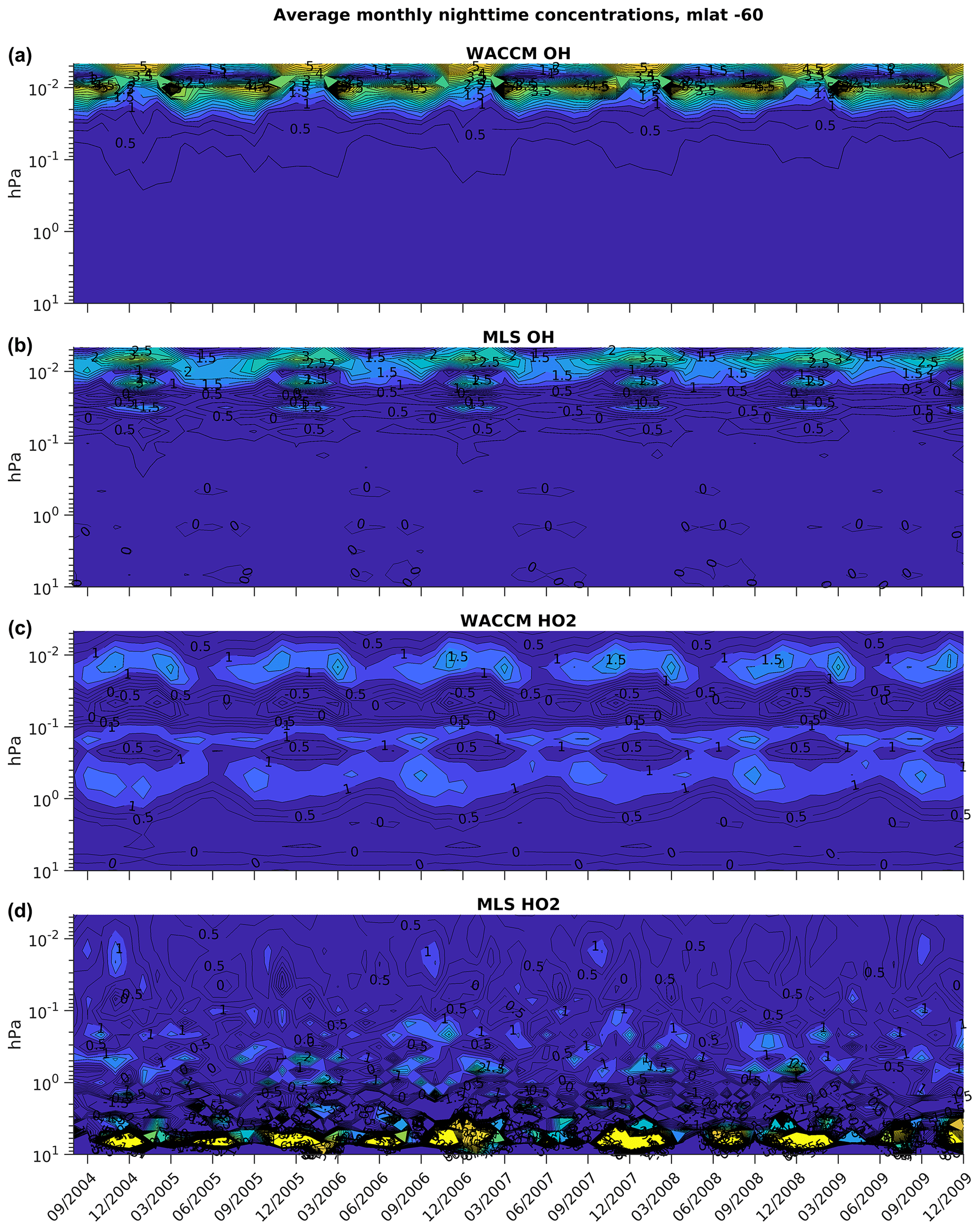
Figure 6 Monthly average nighttime OH and HO₂ concentrations on magnetic latitude 60^∘ S. From (a) to (d): WACCM-D OH; MLS OH; WACCM-D HO₂; MLS HO₂. Concentrations are in units 10⁶ cm⁻³.

Both WACCM-D and MLS show the characteristic OH peak in the mesosphere, produced at night from reactions between atomic hydrogen and O₂. The peak is approximately at the same pressure level of 0.01 hPa, but its magnitude is larger and the seasonal variability is weaker in WACCM-D. In summer, the peak occurs at a higher altitude and is stronger in both WACCM-D and MLS, although the altitude variation is slightly less obvious in MLS data. The MLS OH data also show oscillating minima and maxima in summertimes at 0.1–0.01 hPa, but these may be an artifact of the observations and are not seen in WACCM-D.

For HO₂, WACCM-D shows an upper mesospheric peak with a clear seasonal cycle, coinciding with the OH peak. In addition, there is another clear peak at around 0.5 hPa, with a seasonal cycle that has a minimum in winter and clear maxima in spring and autumn. MLS HO₂ data are noisy, and there are no clear patterns of seasonal variability.

Our WACCM-D/MLS HO₂ comparison results are similar to those by Millán et al. (2015), although it should be noted that they presented the data in geographic coordinates. WACCM-D and MLS clearly produce similar structural patterns. Daytime peak in the mesosphere is stronger in MLS, with potential reasons including model deficiencies in chemistry, solar radiation, and meridional circulation from gravity waves (Millán et al., 2015). Nighttime differences are smaller than during daytime. Overall, the model and observations agree reasonably well, so EPP detection possibilities should be similar – at least in terms of the background level of HO_x.

4.2 SPE thresholds

Figure 7a–c shows all detected nighttime SPE threshold values. As discussed in Sect. 3, correlations ≥0.35 between the square root of the SPE indicator and HO_x data are taken as indication of reasonable thresholds. These correlations are shown in Fig. 7d–f. At higher latitudes in both hemispheres, i.e., at 60–80^∘, the correlations are distinctly high, while at other latitudes there is essentially no correlation. In the polar regions, the nightly threshold values are typically 50–130 $\mathrm{protons}{\mathrm{cm}}^{-\mathrm{2}}{\mathrm{s}}^{-\mathrm{1}}{\mathrm{sr}}^{-\mathrm{1}}$. At magnetic latitude 80^∘ S, the thresholds are lower than elsewhere, i.e., 35–80 $\mathrm{protons}{\mathrm{cm}}^{-\mathrm{2}}{\mathrm{s}}^{-\mathrm{1}}{\mathrm{sr}}^{-\mathrm{1}}$, which would make this latitude band the best for SPE detection. The lower overall background concentration, especially in the SH due to the geomagnetic latitude distribution, makes detection easier, which leads to these lower thresholds. There are, however, larger variations at 80^∘ S as well, due to smaller amount of data available, causing weaker correlations in the MLS observations. Overall, WACCM-D and MLS show similarly distributed threshold values. Comparing the thresholds from OH, SPEs are detected lower into the atmosphere in WACCM-D than MLS data, i.e., from around 80 km down to about 35 and 50 km, respectively. This is seen in both hemispheres, in both thresholds and correlations, and can be explained by the MLS OH data becoming noisier in the stratosphere. In WACCM-D, the thresholds from OH and HO₂ are very consistent, although correlations are weaker in HO₂ in the Southern Hemisphere above 1 hPa.

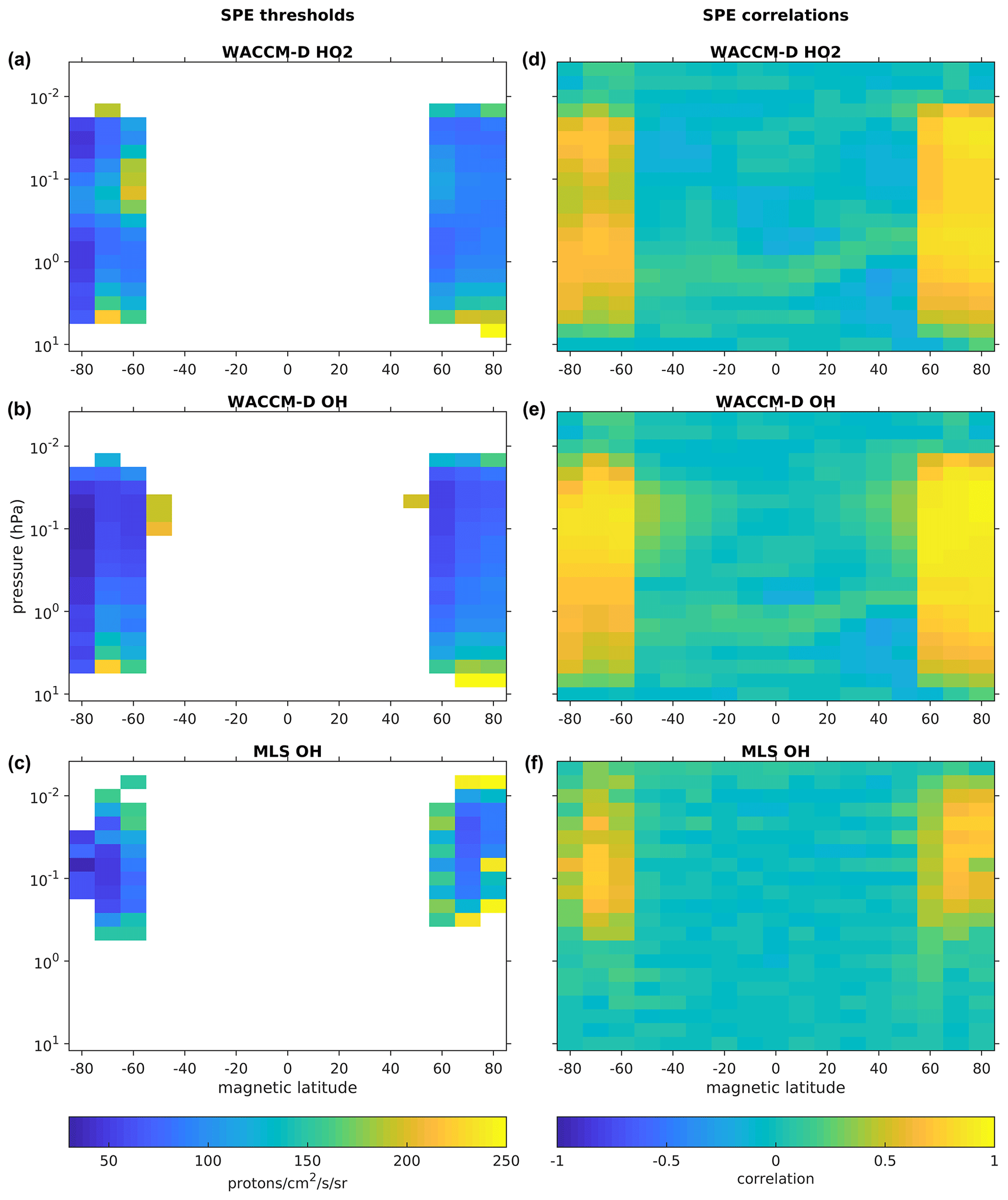
Figure 7 Nighttime SPE indicator thresholds (a–c) and corresponding correlations (d–f). WACCM-D HO₂ (a, d), WACCM-D OH (b, e), and MLS OH (c, f).

Daytime SPE thresholds and correlations are shown in Fig. 8. Again, regions of high correlations are at high latitudes, 60–80^∘, as expected. Because the daytime background concentrations of HO_x are higher at most altitudes, the thresholds can be detected in a more restricted altitude range compared to nighttime. In WACCM-D, the detection can be done at 50–80 km. Both the threshold values and the correlations are very similar for HO₂ and OH data, even more so than at nighttime. For MLS OH, the correlations are overall lower than in WACCM-D, and there is a larger disparity between the NH and SH. No thresholds are detected in the SH, and in the NH, a total of three grid points, all at latitude 80^∘ N, have high enough correlations to qualify as reasonable thresholds. The WACCM-D thresholds vary mostly from 85 to 130 $\mathrm{protons}{\mathrm{cm}}^{-\mathrm{2}}{\mathrm{s}}^{-\mathrm{1}}{\mathrm{sr}}^{-\mathrm{1}}$, though there are many values up to 300 $\mathrm{protons}{\mathrm{cm}}^{-\mathrm{2}}{\mathrm{s}}^{-\mathrm{1}}{\mathrm{sr}}^{-\mathrm{1}}$, while MLS OH thresholds range from 145 to 220 $\mathrm{protons}{\mathrm{cm}}^{-\mathrm{2}}{\mathrm{s}}^{-\mathrm{1}}{\mathrm{sr}}^{-\mathrm{1}}$. Thus, the daytime threshold values are higher than for the nighttime, and there is larger range of values as well.

Figure 8 Daytime SPE indicator thresholds (a–c) and corresponding correlations (d–f). WACCM-D HO₂ (a, d), WACCM-D OH (b, e), and MLS OH (c, f).

We do not include MLS HO₂ in Figs. 7–8 because we could not detect thresholds due to the noisiness of the data. However, the correlations between MLS HO₂ data and the square root of the SPE indicator for both daytime and nighttime are shown in Fig. 9. The correlations are quite uniformly around zero, although there are some larger values seen in the NH high latitudes and altitudes. Nevertheless, no effect of proton precipitation is detectable in the MLS HO₂ data. In the threshold detection analysis, the MLS averaging kernels were not applied to the WACCM-D data. However, we tested their impact and found that the averaging kernels lead to lower correlations overall and higher threshold values, especially at altitudes above 1 hPa. Thresholds could still be detected using WACCM-D data, especially in the NH (not shown).

Figure 9 Correlations between SPE indicator and MLS HO₂ concentrations, showing (a) daytime and (b) nighttime. Due to the low correlations, no threshold values could be detected.

In WACCM-D, the SPE forcing is applied uniformly at geomagnetic latitudes $>{\mathrm{60}}^{\circ }$, and in HO_x, the impact is detected at all the same latitudes. Observations also confirm that the same latitude extent is seen in MLS OH observations at night. Verronen et al. (2007) used MLS OH data to study the latitudinal extent of the proton forcing during the January 2005 SPE, comparing the results to a 1D atmospheric simulation. They found that the lowest geomagnetic latitude affected by the SPE varied between 57 and 64^∘ during the event. This agrees with our results, with SPE impact detected at latitude bins poleward of 55^∘ in the NH and SH. On the other hand, Heino et al. (2019) compared the latitudinal extent of 62 SPEs using cosmic radio noise absorption from a chain of riometer (relative ionospheric opacity meter) observations to those calculated from WACCM-D ionospheric output. They concluded that WACCM-D tends to overestimate the SPE impact at geomagnetic latitudes $>{\mathrm{66}}^{\circ }$. However, Heino et al. (2019) included a large number of smaller events which are expected to affect the highest latitudes only (e.g., Rodger et al., 2006). For the set of events considered by us, the SPE impact seems to cover all geomagnetic latitudes above 60^∘.

The SPE threshold fluxes from our HO_x analysis are of the order of 100 $\mathrm{protons}{\mathrm{cm}}^{-\mathrm{2}}{\mathrm{s}}^{-\mathrm{1}}{\mathrm{sr}}^{-\mathrm{1}}$. Thus, our results are in agreement with a recent simulation study of SPE-driven atmospheric impacts, which suggested little effect from SPEs with a smaller peak flux (Kalakoski et al., 2020). This detection limit means that, of the 130 SPEs recorded in 2004–2018, 36 (28 %) have a peak daily flux large enough for HO_x-based atmospheric detection.

4.3 RBE detection

The thresholds and correlations for nighttime RBE detection are shown in Fig. 10. In general, the HO_x reaction to radiation belt electron precipitation is more limited in altitude and latitude compared to proton precipitation, which can be expected from the spatial extent and energy range of the observed electron fluxes.

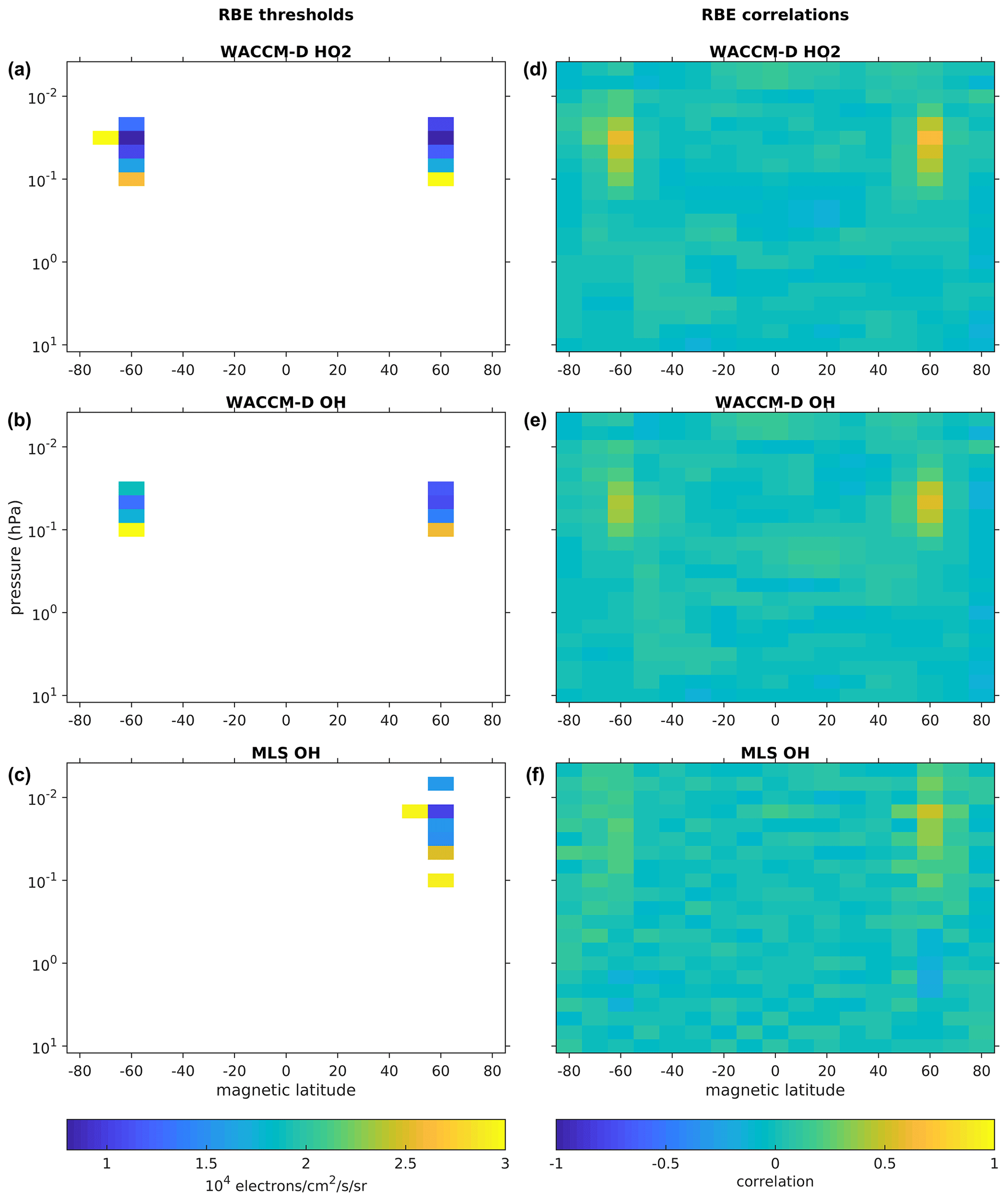
Figure 10 Nighttime RBE indicator thresholds (a–c) and corresponding correlations (d–f). WACCM-D HO₂ (a, d), WACCM-D OH (b, e), and MLS OH (c, f).

Overall, we detect RBE only at latitudes poleward of 60^∘ (NH and SH) and at altitudes from roughly 65 to 75 km. In WACCM-D, the detection threshold is mostly 1.05–2.55×10⁴ $\mathrm{electrons}{\mathrm{cm}}^{-\mathrm{2}}{\mathrm{s}}^{-\mathrm{1}}{\mathrm{sr}}^{-\mathrm{1}}$, with lower values from WACCM-D when using the HO₂ data. With MLS OH data, in the NH the detected RBE threshold values are similar to those with WACCM-D OH but with a slightly larger spread, i.e., 1.00–2.95×10⁴ $\mathrm{electrons}{\mathrm{cm}}^{-\mathrm{2}}{\mathrm{s}}^{-\mathrm{1}}{\mathrm{sr}}^{-\mathrm{1}}$, and cover a wider altitude range from 60 to 80 km. MLS OH seems to show a wider latitude range for detection in the correlations as well, extending over latitudes, 50–70^∘, although RBE can be detected only in one grid point outside 60^∘ N. A possible indication of this wider latitude range can also be seen in the SH in WACCM-D HO₂, where a single threshold value can be detected at 70^∘ S. No thresholds can be found for MLS HO₂ nighttime data, i.e., the situation is the same as for the SPE detection. There are no clear correlations between MLS HO₂ and RBE indicator (not shown). In the daytime, all correlations between the RBE indicator and HO_x concentrations are low. The number of detected daytime RBE indicator threshold values is only two, both with MLS OH (Fig. 11). These thresholds are 2.16 and 2.50×10⁴ $\mathrm{electrons}{\mathrm{cm}}^{-\mathrm{2}}{\mathrm{s}}^{-\mathrm{1}}{\mathrm{sr}}^{-\mathrm{1}}$ at altitudes 0.0147 and 0.0215 hPa, respectively, both at magnetic latitude 70^∘ N.

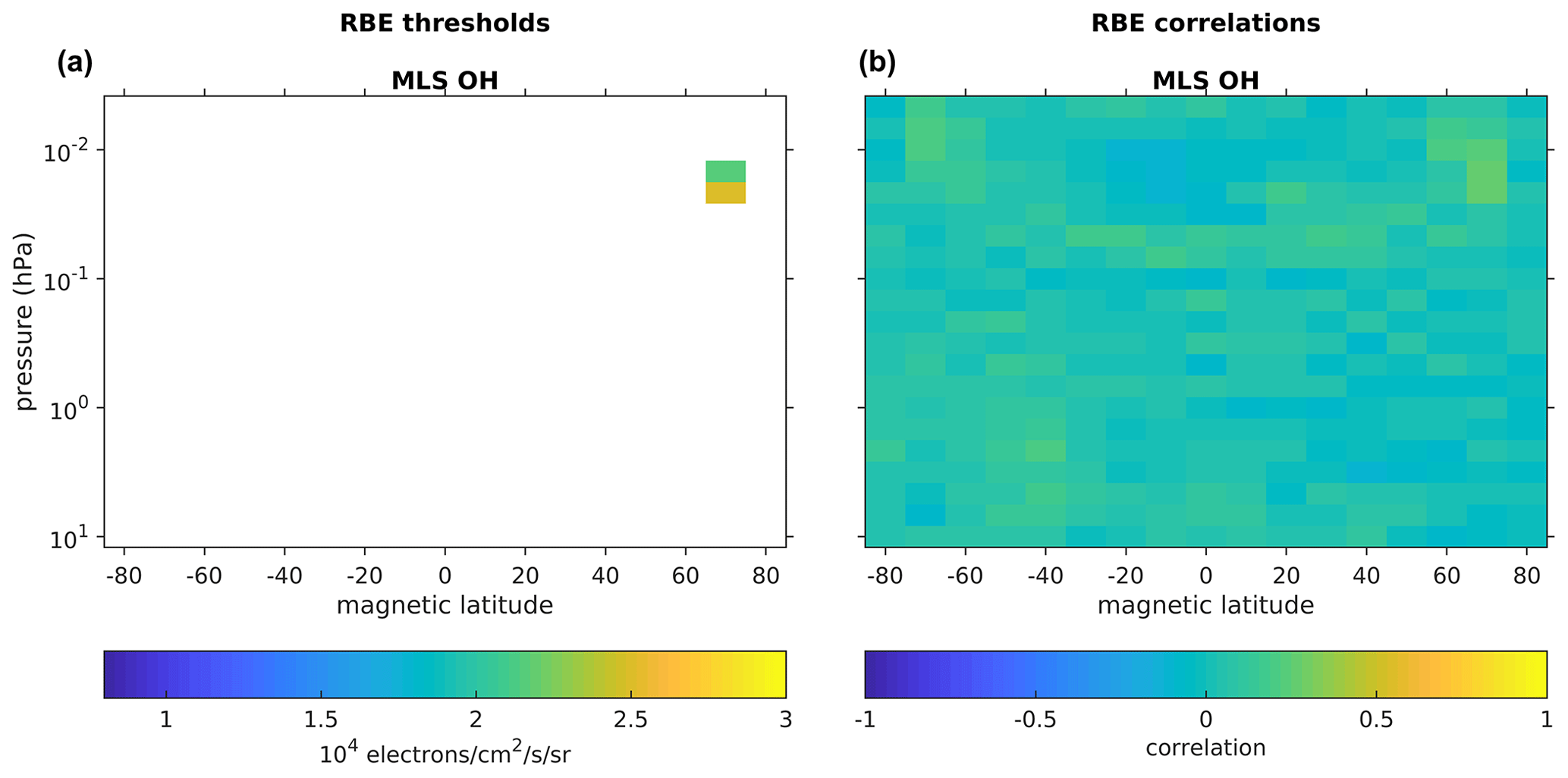
Figure 11 Daytime RBE indicator thresholds (a) and corresponding correlations (b) for MLS OH.

In an attempt to improve some of the results, 5 d averaged data were also examined. A moving 5 d average was calculated from the HO_x data and analyzed, as above, with the SPE and RBE indicators. This was done to remove some of the noise, especially in the MLS HO₂, but the results were not improved. The data smoothing effectively flattened out the daily concentration peaks caused by events, which generally led to slightly lower correlations with the SPE and RBE indicators. Thus, the daily values can be considered an optimal choice for EPP detection, taking into account that a typical SPE/RBE event duration is days.

Although RBE forcing in WACCM-D is applied at geomagnetic latitudes 40–72^∘, the detection in HO_x impact is only seen at 55–65^∘. Unlike the SPE forcing, RBE is not uniform over the latitude range but peaks at the heart of the outer radiation belt (van de Kamp et al., 2016). Thus, only this region can be used to detect the HO_x impact. In the MLS data, i.e., in the correlations shown in Fig. 10, the RBE extent in the NH seems to reach into neighboring bins outside 55–65^∘, although the correlation limit is not exceeded. This could indicate an underestimation in WACCM-D RBE forcing which is driven by the geomagnetic Ap index.

The RBE threshold fluxes are of the order of 10⁴ $\mathrm{electrons}{\mathrm{cm}}^{-\mathrm{2}}{\mathrm{s}}^{-\mathrm{1}}{\mathrm{sr}}^{-\mathrm{1}}$, i.e., 100 times larger fluxes than for SPEs. This is consistent considering that 100 keV electrons ionize about 100 times fewer molecules than 10 MeV protons while penetrating to about the same atmospheric altitude. Considering the time period 2004–2018, there are 192 d, i.e., 3.9 % of all days, which have RBE flux larger than the 10⁴ threshold. Note that our RBE thresholds are an order of magnitude larger than those given by Verronen et al. (2011). Analyzing four large RBE events, they estimated that it is not possible to detect the HO_x impact from electron forcing less than 10–30 counts s⁻¹ as measured by MEPED, and this count rate corresponds to fluxes of 1–3×10³ $\mathrm{electrons}{\mathrm{cm}}^{-\mathrm{2}}{\mathrm{s}}^{-\mathrm{1}}{\mathrm{sr}}^{-\mathrm{1}}$ (Evans and Greer, 2004).

5 Conclusions

In this study, we have used atmospheric HO_x data as a detector of EPP impact in the mesosphere and stratosphere. In a sense, WACCM-D simulations have provided us with the theoretical thresholds for the detection, while MLS observations are the present reality that is affected also by the quality of the measurements.

Overall, SPE impacts can be well detected using average nighttime OH data from MLS. Based on the WACCM-D results, detection should be possible also at daytime and using HO₂ data. In practice, however, the current MLS data do not have good enough signal-to-noise ratio to do this. RBE detection is possible as well but only at nighttime and for more limited altitude and latitude ranges. While the SPE impact can be seen rather uniformly poleward of 60^∘, the RBE impact is focused at 60^∘. As with SPEs, only MLS OH observations can be used for confident RBE detection on a day-by-day basis.

Our analysis shows the extent of SPE atmospheric impacts, down to around 35 and 50 km in WACCM-D and MLS, respectively. The noise in MLS observations likely causes the difference in the altitude extent. Below 50 km altitudes, MLS HO_x cannot be reliably used to detect SPEs. Potentially, however, other species like Cl_x or HNO₃ could provide better SPE detection capabilities in the stratosphere. For example, the simulations of SPE impacts by Kalakoski et al. (2020) showed enhancements in Cl_x and HNO₃ between 1 and 0.01 hPa, lasting around a week, and longer-lasting (20–30 d) effects below the 1 hPa level in HNO₃.

We find thresholds for EPP detection using the GOES > 10 MeV proton fluxes and POES 100–300 keV electron fluxes to be around 50–130 $\mathrm{protons}{\mathrm{cm}}^{-\mathrm{2}}{\mathrm{s}}^{-\mathrm{1}}{\mathrm{sr}}^{-\mathrm{1}}$ and 1.0–2.5 ×10⁴ $\mathrm{electrons}{\mathrm{cm}}^{-\mathrm{2}}{\mathrm{s}}^{-\mathrm{1}}{\mathrm{sr}}^{-\mathrm{1}}$ at nighttime. These flux values have to be exceeded to cause a detectable HO_x impact. This limits the data usability to relatively large events. Note, however, that this does not mean that EPP with smaller fluxes is insignificant for the atmosphere. If applied for longer periods of time, EPP below the threshold limit can cause cumulative impacts on chemically long-lived species like NO_x.

Although the MLS HO₂ data were found to be too noisy for day-to-day EPP detection, they still have great potential for other purposes. For example, studies of solar cycle variability in the mesosphere could greatly benefit from the long time series. Also, it has been shown, e.g., by Jackman et al. (2014), that the MLS HO₂ data are useful when the largest solar proton events are studied.