the Creative Commons Attribution 4.0 License.
the Creative Commons Attribution 4.0 License.
 | 10 Nov 2020
Analysis of different propagation models for the estimation of the topside ionosphere and plasmasphere with an ensemble Kalman filter
David Minkwitz
Michael Schmidt
Eren Erdogan
The accuracy and availability of satellite-based applications, like Global Navigation Satellite System (GNSS) positioning and remote sensing, crucially depend on the knowledge of the ionospheric electron density distribution. The tomography of the ionosphere is one of the major tools for providing links to specific ionospheric corrections and studying and monitoring physical processes in the ionosphere and plasmasphere. In this work, we apply an ensemble Kalman filter (EnKF) approach for the 4D electron density reconstruction of the topside ionosphere and plasmasphere, with the focus on the investigation of different propagation models, and compare them with the iterative reconstruction technique of simultaneous multiplicative column normalized method plus (SMART+). The slant total electron content (STEC) measurements of 11 low earth orbit (LEO) satellites are assimilated into the reconstructions. We conduct a case study on a global grid with altitudes between 430 and 20 200 km, for two periods of the year 2015, covering quiet to perturbed ionospheric conditions. Particularly the performance of the methods for estimating independent STEC and electron density measurements from the three Swarm satellites is analysed. The results indicate that the methods of EnKF, with exponential decay as the propagation model, and SMART+ perform best, providing, in summary, the lowest residuals.
- Article
(4968 KB) - Full-text XML
- BibTeX
- EndNote


The ionosphere is the charged part of the upper atmosphere extending from about 50 to 1000 km and going over in the plasmasphere. The characteristic property of the ionosphere is that it contains sufficient free electrons to affect the propagation of trans-ionospheric radio signals from telecommunication, navigation or remote sensing satellites by refraction, diffraction and scattering. Therefore, knowledge of the 3D electron density distribution and its dynamics are of practical importance. Around 50 % of the signal delays or range errors of L-band signals used in the Global Navigation Satellite System (GNSS) originate from altitudes above the ionospheric F2 layer, consisting of topside ionosphere and plasmasphere (see Klimenko et al., 2015; Chen and Yao, 2015). So far, especially the topside ionosphere and plasmasphere, has not been well described.
The choice of the ionospheric correction model has an essential impact on the accuracy of the estimated ionospheric delay and its uncertainty. A widely used approach for ionospheric modelling is the single-layer model, whereby the ionosphere is projected onto a 2D spherical layer, typically located between 350 and 450 km. However, 2D models are usually not accurate enough to support high-accuracy navigation and positioning techniques in real time (see, for example, Odijk, 2002; Banville, 2014). More accurate and precise positioning is achievable by considering the ionosphere as a 3D medium. There are several activities in the ionosphere community aiming to describe the mean ionospheric behaviour by the development of 3D electron density models based on long-term historical data. Two widely used models are the International Reference Ionosphere (IRI) model (see Bilitza et al., 2011) and the NeQuick model (see Nava et al., 2008).
Since those models represent a mean behaviour, it is essential to update them by assimilating actual ionospheric measurements. There have been a variety of approaches developed and validated for ionospheric reconstruction by the combination of actual observations with an empirical or a physical background model. Hernandez-Pajares et al. (1999) present one of the first GNSS-based data-driven tomographic models, which considers the ionosphere as a grid of 3D voxels, and the electron density within each voxel is computed as a random walk time series. The voxel-based discretization of the ionosphere is further used, for instance, in Heise et al. (2002), Wen et al. (2007), Gerzen and Minkwitz (2016), Gerzen et al. (2017) and Wen et al. (2020). These authors reconstruct the 3D ionosphere by algebraic iterative methods. An alternative is to estimate the electron density as a linear combination of smooth and continuous basis functions, like, for example, spherical harmonics (SPHs; Schaer, 1999), B-splines (Schmidt et al., 2008; Zeilhofer, 2008; Zeilhofer et al., 2009; Olivares-Pulido et al., 2019), B-splines and trigonometric B-splines (Schmidt et al., 2015), B-splines and Chapman functions (Liang et al., 2015, 2016), and empirical orthogonal functions and SPHs (Howe et al., 1998).
Besides the algebraic methods, other techniques benefitting from information on spatial and temporal covariance information, such as optimal interpolation, the Kalman filter, 3D and 4D variational techniques and kriging, are applied to update the modelled electron density distributions (see Howe et al., 1998; Angling et al., 2008; Minkwitz et al., 2015 and 2016; Nikoukar et al., 2015; Olivares-Pulido et al., 2019).
Moreover, there are approaches based on physical models which combine the estimation of the electron density with physically related variables, such as neutral winds or the oxygen / nitrogen ratio (see Wang, et al., 2004; Scherliess et al., 2009; Lee et al., 2012; Lomidze et al., 2015; Schunk et al., 2004, 2016; Elvidge and Angling, 2019).
In general, the majority of data available for the reconstruction of the ionosphere and plasmasphere are slant total electron content (STEC) measurements, i.e. the integral of the electron density along the line of sight between the GNSS satellite and receiver. Often, STEC measurements provide limited vertical information, and hence, the modelling of the vertical the electron density distribution is hampered (see, for example, Dettmering, 2003). The estimation of the topside ionosphere and plasmasphere poses a particular difficulty since direct electron density measurements are rare, and low plasma densities at these high altitudes contribute only marginally to the STEC measurements. Ground-based STEC measurements are especially dominated by electron densities within and below the characteristic F2 layer peak. Consequently, information about the plasmasphere is difficult to extract from ground-based STEC measurements (see, for example, Spencer and Mitchell, 2011). Thus, in the presented work, we concentrate on the modelling of the topside part of the ionosphere and plasmasphere and utilize only the space-based STEC measurements.
In this paper, we introduce an ensemble Kalman filter (EnKF) to estimate the topside ionosphere and plasmasphere based on space-based STEC measurements. The propagation of the analysed state vector to the next time step within a Kalman filter is a key challenge. The majority of the approaches, working with EnKF variants, use physics-based models for the propagation step (see, for example, Elvidge and Angling, 2019; Codrescu et al., 2018; Lee et al., 2012). In our work, we investigate the question of how the propagation step can be realized if a physical model is not available or if the usage of a physical model is rejected as computationally time consuming. We discretize the ionosphere and the plasmasphere below the GNSS orbit height by 3D voxels, initialize them with electron densities calculated by the NeQuick model and update them with respect to the data. We present different methods for how to perform the propagation step and assess their suitability for the estimation of electron density. For this purpose, a case study of quiet and perturbed ionospheric conditions in 2015 is conducted to investigate the capability of the estimates to reproduce assimilated STEC and to reconstruct independent STEC and electron density measurements.
We have organized the paper as follows: Sect. 2 describes the EnKF with the different propagation methods and the generation of the initial ensembles by the NeQuick model. Section 3 outlines the validation scenario with the applied data sets. Section 4 presents the obtained results. Finally, we conclude our work in Sect. 5 and provide an overview of the next steps.
2.1 Formulation of the underlying inverse problem
Information about the STEC along the satellite-to-receiver ray path s can be obtained from multi-frequency GNSS measurements. In detail, STEC is a function of the electron density Ne along the ray path s, given by the following:
where is the unknown function describing the electron density values depending on altitude h, geographic longitude λ and latitude φ.
The discretization of the ionosphere by a 3D grid and the assumption of a constant electron density function within a fixed voxel allows the transformation of Eq. (1) into a linear system of equations as follows:
where y is the (m×1) vector of the STEC measurements, x is the vector of unknown electron densities with xi=Nei equal to the electron density in the voxel i, hsi is the length of the ray path s in the voxel i, and r is the vector of measurement errors assumed to be Gaussian-distributed , with the expectation and covariance matrix R.
2.2 Background model
As a regularization of the inverse problem in Eq. (2), a background model often provides the initial guess of the state vector x. In this study, we apply the NeQuick model (version 2.0.2). The NeQuick model was developed at the International Centre for Theoretical Physics (ICTP) in Trieste, Italy, and at the University of Graz, Austria (see Hochegger et al., 2000; Radicella and Leitinger, 2001; Nava et al., 2008). The daily solar flux index of F10.7 is used to drive the NeQuick model.
2.3 Analysis step of the EnKF
We apply EnKF to solve the inverse problem defined in Sect. 2.1. Evensen (1994) introduces the EnKF as an alternative to the standard Kalman filter (KF) in order to cope with the non-linear propagation dynamics and the large dimension of the state vector and its covariance matrix. In an EnKF, a collection of realizations, called ensembles, represent the state vector x and its distribution.
Let be a (K×N) matrix in which the columns are the ensemble members, ideally following the a priori distribution of the state vector x. Furthermore, the observations collected in y are treated as random variables. Therefore, we define an (m×N) ensemble of observations , with and a random vector ϵi from the normal distribution N(0, R).
We define the ensemble covariance matrix P around the ensemble mean as follows:
In the analysis step of the EnKF, the a priori knowledge of the state vector x and its covariance matrix P is updated by the following:
where the matrix Xa represents the a posteriori ensembles and, hence, the a posteriori state vector.
For the propagation of the analysed solution to the next time step, we test different propagation models described in Sect. 2.4. In order to generate the initial ensembles Xf(t0), we use the NeQuick model and describe the procedure in Sect. 2.5. Keeping in mind that we have to deal with an extremely large state vector (details are presented in Sect. 3.1), the important advantage of the EnKF for the present study is that there is no need to explicitly calculate the ensemble covariance matrix (see Eq. 3). Instead, to perform the analysis step in Eq. (4), we follow the implementation suggested by Evensen (2003).
2.4 Considered models for the propagation step of the EnKF
In this section, we introduce different models to propagate the analysed solution to the next time step. With all of them, we propagate the ensembles 20 min in time. Generally, these propagation models can be described as . In the following subsections, we outline possible choices of the model F, the systematic error WF and the process noise ΩF.
Note that, beyond the presented methods, we had additionally tested a propagation model based on persistence, i.e. . Already after a time period of about 24 h, this method had shown unreasonable effects in the reconstructions, like a completely misplaced equatorial crest region.
2.4.1 Method 1: rotation
The method rotation assumes that, in geomagnetic coordinates, the ionosphere remains invariant in space while the Earth rotates below it (see Angling and Cannon, 2004). Thus, we propagate the analysed ensemble Xa(tn) from time tn to the next time step tn+1 by the following:
To calculate rot(Xa(tn)), the geomagnetic longitude is changed, corresponding to the evolution time , i.e. 5∘ of longitude per 20 min. Wrot denotes the systematic error introduced by approximation of the true propagation of Xf by a simple rotation. We tested the following estimation of Wrot here:
with
where xb is the electron density vector calculated by the NeQuick model and ϵ1×N is a (1×N) matrix of ones. The division in the second equation is element wise. The ratio of ratioRot(tn+1) in Eq. (7) represents the relative error introduced by the application of rot(xb(tn)) instead of xb(tn+1). In this way, we obtain, in Eq. (6), an approximation of the mean error introduced by the approximation of the true state at time tn+1 by the rotation of the true state at time tn. The factor has been chosen empirically as the result of an internal validation not presented within this paper.
2.4.2 Method 2: exponential decay
Here we assume the electron density differences between the voxels of the analysis and the background model to be a first-order Gauss–Markov sequence. These differences are propagated in time by an exponential decay function (see Nikoukar et al., 2015; Bust and Mitchell, 2008; Gerzen et al., 2015).
where Xb(t) is the ensemble of electron density vectors calculated by the NeQuick model for the time t, as described in Sect. 2.5, , , and τ denotes the temporal correlation parameter chosen here as being 3 h.
Note that, similar to the method described here, we also tested the application of rot(Xa(tn)−Xb(tn)) instead of [Xa(tn)−Xb(tn)] in Eq. (8). The results were similar and are therefore not presented here.
2.4.3 Method 3: rotation with exponential decay
For the third method, we define the propagation model as a combination of the propagation models described in the previous subsections, in particular, as the following:
The systematic error W is estimated as follows:
Thereby, f and Wrot are defined as in the two previous sections. The factor is, thereby, again chosen empirically. The process noise Ωexp is assumed to be white, with . Here the matrix Ωrot consists of random realizations of the distribution N(0, Σrot) with the following:
where ratioi increases continuously, depending on the altitude of the voxel i from for lower altitudes to for the higher altitudes (chosen empirically), and E(Rot(Xa(tn))) denotes the ensemble mean vector. Equations (9) and (11) can be interpreted as follows: for the chosen time step of 20 min, the standard deviation of the time model error regarding the voxel i is equal to , varying between 0.5 % and 1 % of the corresponding analysed electron density in the voxel i. In detail, we generate, at each time step, a new vector , with , and calculate the ith row of Ωrot.
The matrix Qexp(tn+1) consists of random realizations (different for each time step) consistent with the a priori covariance matrix L of the errors of the background xb(tn+1) (see Howe and Runciman, 1998). In detail, this means that the a priori covariance is assumed to be diagonal, and Lii equals the square of 1 % of the corresponding background model value. Then the ith row of Qexp is calculated by Eq. (13) as follows:
2.5 Generation of the ensembles
In order to generate the ensembles, we vary the F10.7 input parameter of the NeQuick model (see Sect. 2.2). First, we analysed the sensitivity of the NeQuick model to F10.7. Based on the results, we calculate a vector F10.7(t) of the solar radio flux index, with and at time t. The vector F10.7 serves as input for the NeQuick model to calculate the 100 ensembles of Xb during the considered period and the initial guess of the electron densities Xf(t0).
An example of the variation of the generated ensembles is provided by Fig. 1. Particularly, we show, in this figure, the distribution of the differences between the ensemble of electron densities Xb(t) and the NeQuick model values for the day of year (DOY) 041 and 076. The residuals are depicted for a selected altitude and chosen universal times (UTs) and are presented through different colours (see the subfigure history). In addition, the mean, the standard deviation (SD) and the root mean square (RMS) of the residuals are presented in the subplots.
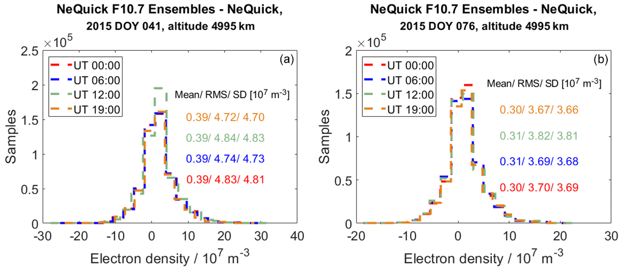
Figure 1The distribution of the ensemble residuals for a chosen altitude and selected universal times (UTs), for all latitudes and longitudes, with panel (a) showing the day of the year (DOY) 041 and (b) showing DOY 076.
2.6 Provision of a benchmark by the simultaneous multiplicative column normalized method plus (SMART+)
In order to provide a benchmark for the described methods, we apply SMART+ as an additional reconstruction technique. The simultaneous multiplicative column normalized method plus (SMART+) is a combination of an iterative simultaneous multiplicative column normalized method (SMART; see Gerzen and Minkwitz, 2016) and a 3D successive correction method (3D SCM) (see, for example, Kalnay, 2011; Gerzen and Minkwitz, 2016). As a first step, SMART distributes the STEC measurements among the electron densities in the ray-path-intersected voxels. For a voxel i, the multiplicative innovation is calculated as a weighted mean of the ratios between the actual measurements and the currently expected measurements. The weights are given by the length of the ray path corresponding to the measurement in the voxel i divided by the sum of lengths of all rays crossing the voxel i. Consequently, only voxels intersected by at least one measurement are innovated during the SMART procedure. Thereafter, assuming non-zero correlations between the ray path intersected voxels and those not intersected by any STEC, an extrapolation is done from intersected to not intersected voxels. For this purpose, one iteration of the 3D SCM is applied. For more details, we refer readers to Gerzen and Minkwitz (2016) and Gerzen et al. (2017).
For SMART+, the number of iterations at each time step is set to 25, and the correlation coefficients are chosen as described in Gerzen and Minkwitz (2016). For each time step, SMART+ reconstructs the electron densities based on the background model (here NeQuick) and the currently available measurements. In other words, there is no propagation of the estimated electron densities from a time step tn to the time step tn+1.
Within this study, the EnKF with different propagation methods is applied and validated for the tomography of the topside ionosphere and plasmasphere. Two periods with quiet (DOY 041–059 in 2015) and perturbed (DOY 074–079 in 2015) ionospheric conditions are analysed. In this scope, we investigate the ability to reproduce assimilated STEC and to estimate independent STEC measurements and in situ electron density measurements of the Swarm Langmuir probes (LPs). In addition, we apply the tomography approach SMART+ (see Sect. 2.6) to provide a benchmark.
3.1 Reconstruction area
We estimate the electron density over the entire globe, with a spatial resolution of 2.5∘ in geodetic latitude and longitude. Altitudes between 430 and 20 200 km are reconstructed where the resolution equals 30 km for altitudes from 430 to 1000 km and decreases exponentially with increasing altitude for altitudes above 1000 km, i.e. 42 altitudes in total. Consequently, the number of unknowns is K=217 728. The temporal resolution Δt is set to 20 min.
3.2 Ionospheric conditions in the considered periods
We use the solar radio flux of F10.7, the global planetary 3 h index Kp and the geomagnetic disturbance storm time (DST) index to characterize the ionospheric conditions during the periods of DOY 041–059 and DOY 074–079 in 2015. In the February period (DOY 041–059 in 2015), the ionosphere is evaluated as being quiet, with F10.7 solar flux unit (sfu) range between 108 and 137s, a Kp index below 6 (on 2 d between 4 and 6; below 4 during the rest of the period) and DST values between 20 and −60 nT. The period on 17 March (DOY 076) 2015 is known as the St Patrick's Day storm. The F10.7 value equals ∼ 116 sfu on DOY 075 and ∼ 113 sfu on DOY 076, the Kp index is below 5 on DOY 075 and increases to 8 on DOY 076, and DST drops down to −200 nT on DOY 076.
3.3 Data
3.3.1 STEC measurements
As input for the tomography approaches and for the validation, we use space-based calibrated STEC measurements of the following low earth orbit (LEO) satellite missions: COSMIC, Swarm, TerraSAR-X, MetOpA and MetOpB and GRACE. Please note that, in 2015, the orbit height of the COSMIC and MetOp satellites was ∼ 800 km, the orbit height of the Swarm B and TerraSAR-X satellites was ∼ 500 km, and the Swarm C satellite was ∼ 460 km. The STEC measurements of Swarm A and GRACE are used for the validation only. The Swarm A satellite flew side by side with the Swarm C satellite at around 460 km height. The height of the GRACE orbit was around 430 km. All satellites flew at almost polar orbits. More information about the LEO satellites may be found on the following web pages:
-
COSMIC, available at: https://www.nasa.gov/directorates/heo/scan/services/missions/earth/COSMIC.html (last access: 2 November 2020).
-
Swarm, available at: https://www.esa.int/Applications/Observing_the_Earth/Swarm (last access: 2 November 2020).
-
TerraSAR-X, available at: https://earth.esa.int/web/eoportal/satellite-missions/t/terrasar-x (last access: 2 November 2020).
-
MetOpA and MetOpB, available at: https://directory.eoportal.org/web/eoportal/satellite-missions/m/metop (last access: 2 November 2020).
-
GRACE, available at: https://www.nasa.gov/mission_pages/Grace/index.html (last access: 2 November 2020).
The STEC measurements of the Swarm satellites are available at https://swarm-diss.eo.esa.int/, last access: 2 November 2020, and the STEC measurements of the other satellite missions are available at http://cdaac-www.cosmic.ucar.edu/cdaac/tar/rest.html, last access: 2 November 2020. Both data providers also supply information on the accuracy of the STEC data. We utilize this information to fill the covariance matrix R of the measurement errors. The collected STEC data are checked for plausibility before the assimilation.
3.3.2 In situ electron density measurements from the Swarm Langmuir probes
The LPs on board the Swarm satellites provide in situ electron density measurements, with a time resolution of 2 Hz. For the present study, the LP in situ data are acquired from https://swarm-diss.eo.esa.int/, last access: 2 November 2020. In addition, further information on the preprocessing of the LP data is made available on this website.
Lomidze et al. (2018) assess the accuracy and reliability of the LP data (December 2013 to June 2016) by nearly coincident measurements from low- and mid-latitude incoherent scatter radars, low-latitude ionosondes and COSMIC satellites, which cover all latitudes. The comparison results for each Swarm satellite are consistent across these different measurement techniques. The results show that the Swarm LPs underestimate the electron density systematically by about 10 %.
In this section, the different methods are presented with the following colour code: blue for the method rotation, green for the method exponential decay, light blue for the method rotation with exponential decay and magenta for NeQuick and red for SMART+. The legends in the figures are the following: “Rot” for the method rotation, “Exp” for the method exponential decay and “Rot and Exp” for the method rotation with exponential decay.
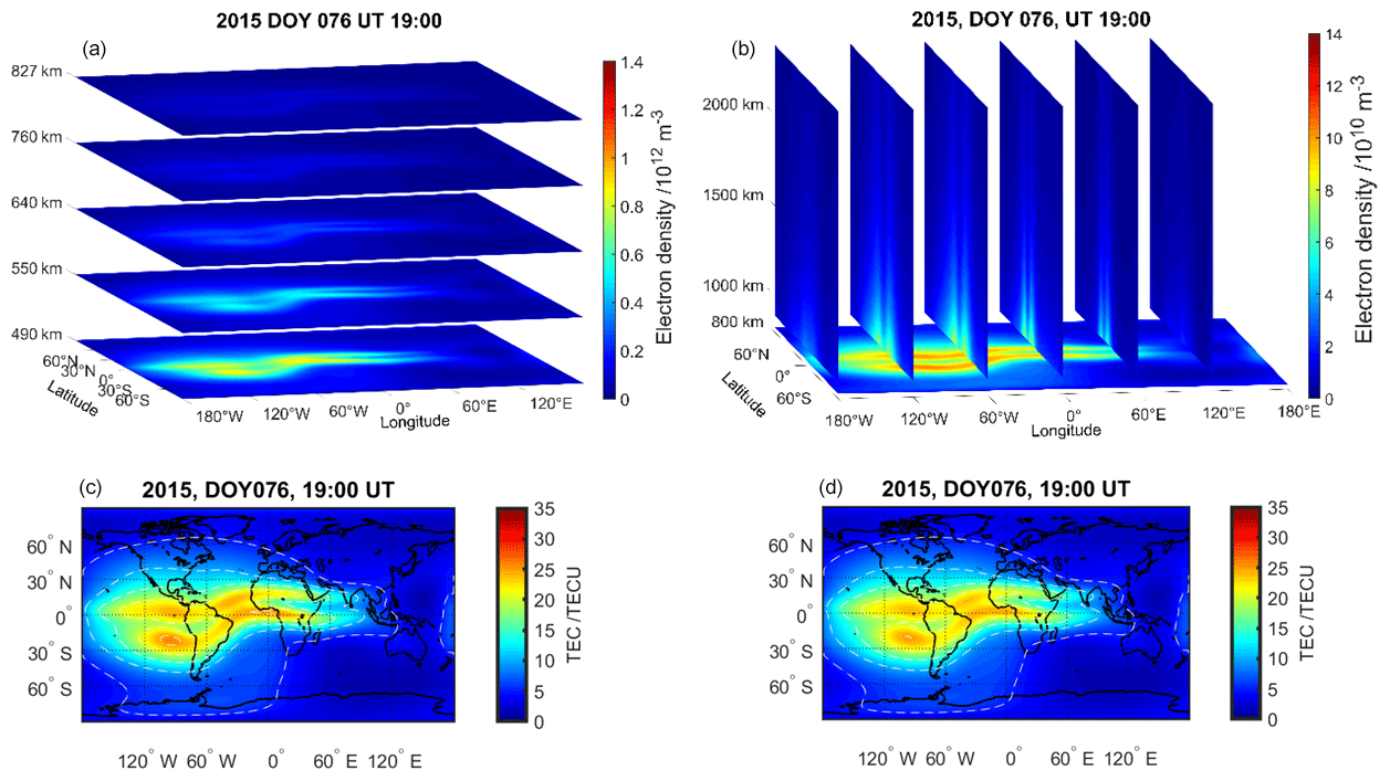
Figure 2Rotation with exponential decay reconstructed electron density, represented by layers at different heights between 490 and 827 km (a) and at chosen longitudes for altitudes between 827 and 2400 km (b). The vertical total electron content (TEC) map deduced from the reconstructed (c) and NeQuick-modelled (d) 3D electron density in the altitude range between 450 and 20 200 km.
4.1 Reconstructed electron densities
At the end of each EnKF analysis step, we have, for each of the considered methods, 100 ensembles representing the electron density values within the voxels. The EnKF-reconstructed electron densities are then calculated as the ensemble mean. Figure 2a and b present the electron densities reconstructed by the method rotation with exponential decay, i.e. , for tn, corresponding to DOY 076 at 19:00 UT. Figure 2a shows the horizontal layers of the topside ionosphere at different heights between 490 and 827 km. Figure 2b illustrates the plasmasphere for altitudes between 827 and 2400 km at selected longitudes. Figure 2c and d show the vertical total electron content (VTEC) maps deduced from the 3D electron density in the considered altitude range between 430 and 20 200 km, where Fig. 2c represents the reconstructed values, and Fig. 2d shows the VTEC calculated from the NeQuick model. It is observed that the reconstructed VTEC values are slightly higher than the ones of the NeQuick model.

Figure 3Method rotation reconstructed electron density represented by layers at different heights between 490 and 827 km (a), and a vertical TEC map deduced from the reconstructed 3D electron density in the altitude range between 450 and 20 200 km (b).
Figure 3 displays the electron density layers reconstructed by the method rotation, i.e. , for tn, corresponding to DOY 076 at 19:00 UT. Again, reconstructed electron densities at heights between 490 and 827 km (Fig. 3a) and the corresponding VTEC map deduced from the reconstructed 3D electron density (Fig. 3b) are depicted. All reconstructed values seem to be plausible, showing, as expected, the crest region, low electron densities in the polar regions, etc. The method rotation delivers much higher values than the NeQuick model (see Fig. 2). In Fig. 4, we take a closer look at the differences between the modelled and reconstructed electron densities.
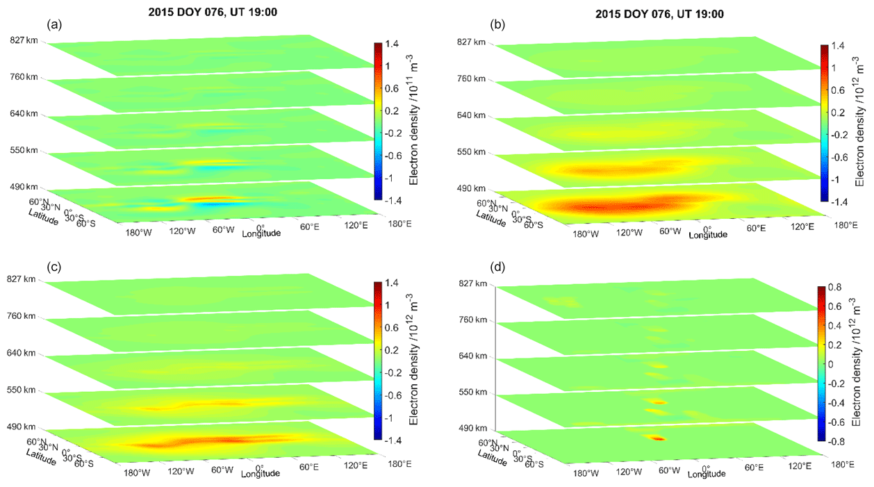
Figure 4Reconstructed minus NeQuick-modelled electron density represented by layers at different heights between 490 and 827 km. (a) Rotation with exponential decay. (b) Rotation. (c) Exponential decay. (d) SMART+.
In the following, we discuss Figs. 4–7 in order to understand the deviations between the reconstructions produced by the different methods. In Fig. 4, the differences between the reconstructed and the modelled electron densities, i.e. E(Xa(tn))−xb(tn), are shown for all methods, namely rotation with exponential decay, rotation, exponential decay and SMART+ (see Fig. 4a–d) on DOY 076 at 19:00 UT. In addition, Fig. 5 expresses these differences in percent. Please note the different ranges of the colour bars for the subfigures. Figure 6 illustrates the orbits of the LEO satellites for the STEC measurements used for the reconstructions on DOY 076, at 19:00 UT (Fig. 6a) and the corresponding ground track (Fig. 6b). The highest differences are observed for the methods of rotation and exponential decay, whereas the method rotation with exponential decay yields the smallest differences. Furthermore, as expected, the EnKF approaches provide smooth and coherent patterns of differences in the ionization. On the contrary, the complementary approach of SMART+ has rather small patterns in areas where measurements are available and falls back to the background model in areas without measurements in the surroundings. In this context, the correlation lengths between the electron densities are of importance. These correlation lengths are set empirically in SMART+, whereas EnKF establishes them automatically, i.e. without setting or estimating them explicitly as, for instance, in SMART+ or kriging approaches. For a comprehensive evaluation of the quality of the different reconstructions in the context of the used correlation lengths, future analyses with further validation data and dependence on the coincidences between the measurement geometry and the geometry of the validation data set are necessary.
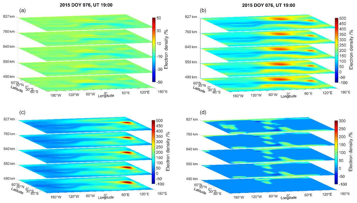
Figure 5Differences between reconstructed and NeQuick-modelled electron density in percent, represented by layers at different heights between 490 and 827 km. (a) Rotation with exponential decay. (b) Rotation. (c) Exponential decay. (d) SMART+.
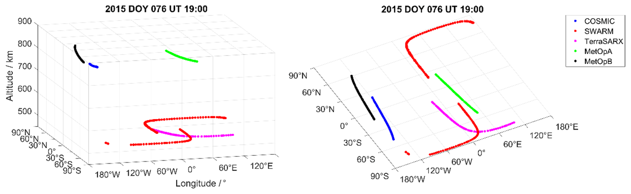
Figure 6The locations of the LEO satellites for the STEC measurements used in the reconstruction.
Taking into account the differences in Fig. 5, for instance around 120∘ E, and the measurement geometry in Fig. 6, it is evident that the estimates of the EnKF are not only based on the current measurements but also on a priori information obtained from assimilations before DOY 076 in 2015 at 19:00 UT. This is, of course, not the case for SMART+.
In order to supplement the understanding of the differences between the propagation methods, Fig. 7a, c and e present the differences , and the percentage differences are shown in Fig. 7b, d and f for tn corresponding to DOY 076 at 19:00 UT. Particularly, the methods (from top to bottom) of rotation with exponential decay, rotation and exponential decay are presented. The differences for the methods rotation and rotation with exponential decay clearly indicate the rotation of the crest region (see also Fig. 3). The method rotation with exponential decay works less rigorously in the rotation than the method rotation since it is anchored by the background model, and the rotation of the differences is damped by the exponential decay function; see Eq. (9). Contrary to these two methods, the method of exponential decay tries to propagate the difference Xa(tn)−Xb(tn) to the next time step and add it to the background Xb(tn+1). Hence, we observe in Fig. 7e a similar pattern to that seen in the corresponding subplot of Fig. 4c.

Figure 7(a, c, e) Differences between the forecasted and analysed electron densities, represented by layers at different heights between 490 and 827 km. (b, d, f) Differences in percent. (a, b) Method rotation with exponential decay. (c, d) Rotation. (e, f) Exponential decay.
In conclusion, the different behaviour of the propagation methods, in combination with the sparse measurement geometry, might serve as an explanation for the substantial differences observed in the VTEC maps shown in Figs. 2 and 3.
4.2 Plausibility check by comparison with assimilated STEC
In this section, we check the ability of the methods to reproduce the assimilated STEC measurements. For that purpose, we calculate STEC along a ray path, j, for all ray path geometries using the estimated 3D electron densities, denoted as , and compare them with the measured STEC, , used for the reconstruction. Then, the mean deviation ΔSTEC between the measurements and the estimate is calculated for each of the considered methods according to the following:
where m is the number of assimilated measurements. ΔSTEC is calculated at each epoch tn. In terms of the notation used for the Eqs. (1)–(4), we can reformulate the above formula for the mean deviation as follows:
Furthermore, we consider the RMS of the deviations, in detail, as follows:
To calculate ΔSTEC and RMS, the same measurements are used as for the reconstruction. In this sense, the results presented in Figs. 8–12 serve as a plausibility check, testing the ability of the methods to reproduce the assimilated TEC.
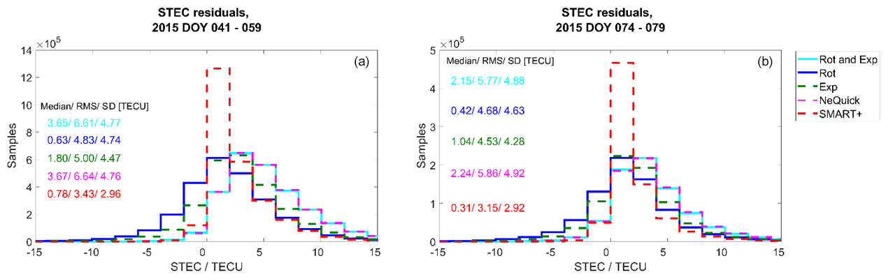
Figure 8Plausibility check of the residuals calculated as measured STEC minus estimated STEC. (a) Residuals of the quiet period and (b) for the perturbed period.
Figure 8a and b depict the distribution of the residuals for the quiet period and for the perturbed period respectively. The corresponding residual median, standard deviation (SD) and root mean square (RMS) values are also presented in the Fig. 8. It is worth mentioning here that, during the quiet period, the measured STEC is below 150 total electron content unit (TECU). For all DOYs of the perturbed period, except for DOY 076, the measured STEC is below ∼ 130 TECU. On DOY 076, the STEC values rise up to 370 TECU.
The NeQuick model seems to underestimate the measured topside ionosphere and plasmasphere STEC during both periods. During both periods, SMART+ seems to perform best, followed by the method rotation. However, rotation produces higher SD and RMS values. Compared to the NeQuick residuals, SMART+ is able to reduce the median of the residuals by up to 86 % during the perturbed period and up to 79 % during the quiet period. The RMS is reduced by up to 48 % and the SD by up to 41 %. Rotation reduces the NeQuick median by up to 83 % and the RMS by up to 27 %, and the SD value is almost on the same level as for NeQuick. The method exponential decay is able to decrease the median of the NeQuick residuals by up to 54 %, the RMS by up to 25 % and the SD values by up to 13 %. The method rotation with exponential decay performs similarly to the NeQuick model. The latter could indicate that the parameters chosen for the error terms and weighting in Eq. (9) could still be improved, although an extensive validation of these parameters was performed prior to the analyses presented in this paper, and the best configuration was selected.
Interestingly, the median values are higher during the quiet period, while the SD values are on the same level when compared between perturbed and quiet periods. The reason, therefore, is probably that the assimilated STEC values have, on average, lower magnitude during the days in the perturbed period compared to those during the quiet period (which explains the lower median), except for the storm on DOY 076, while on DOY 076 they are significantly higher (which explains the comparable SD).
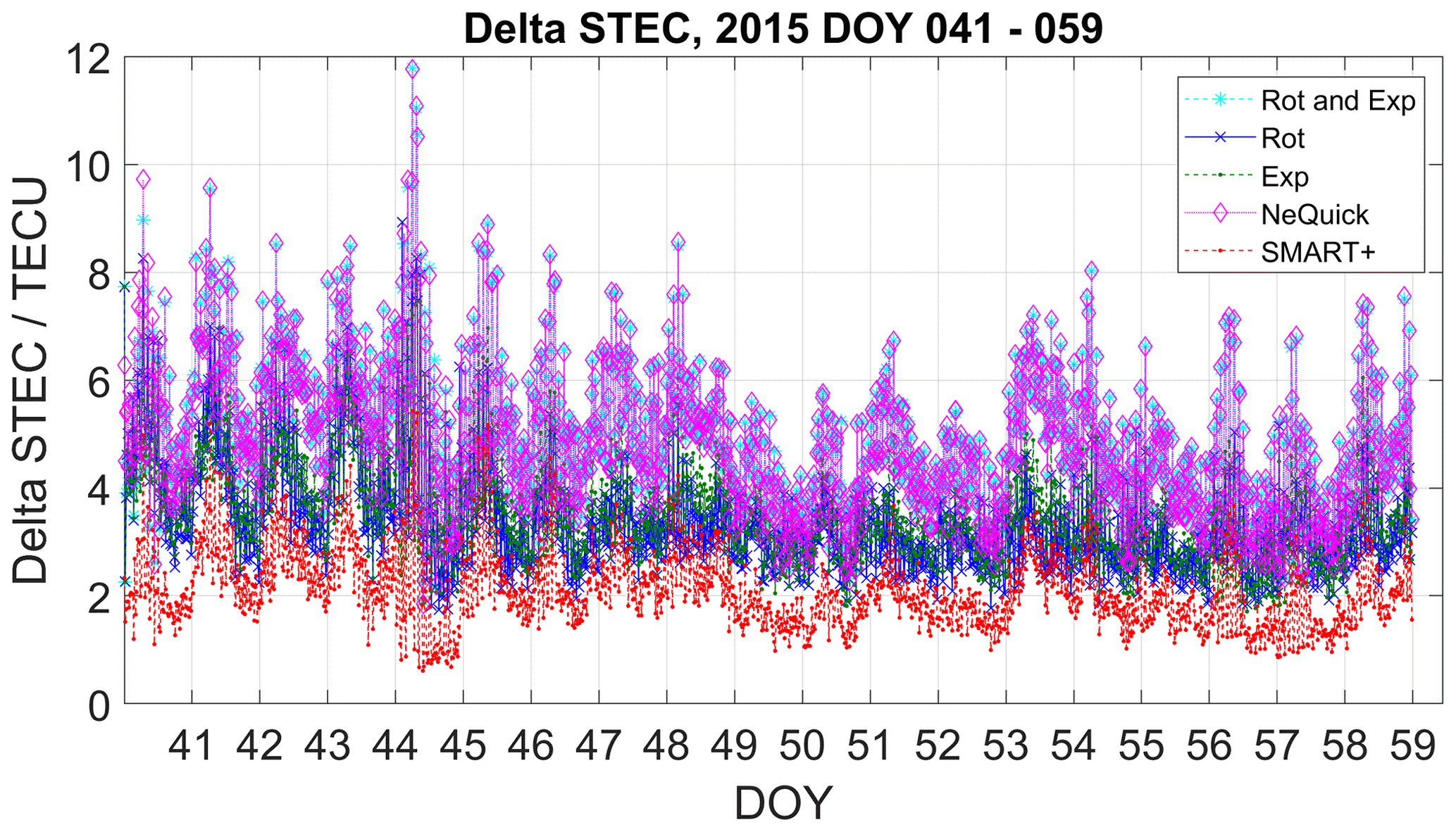
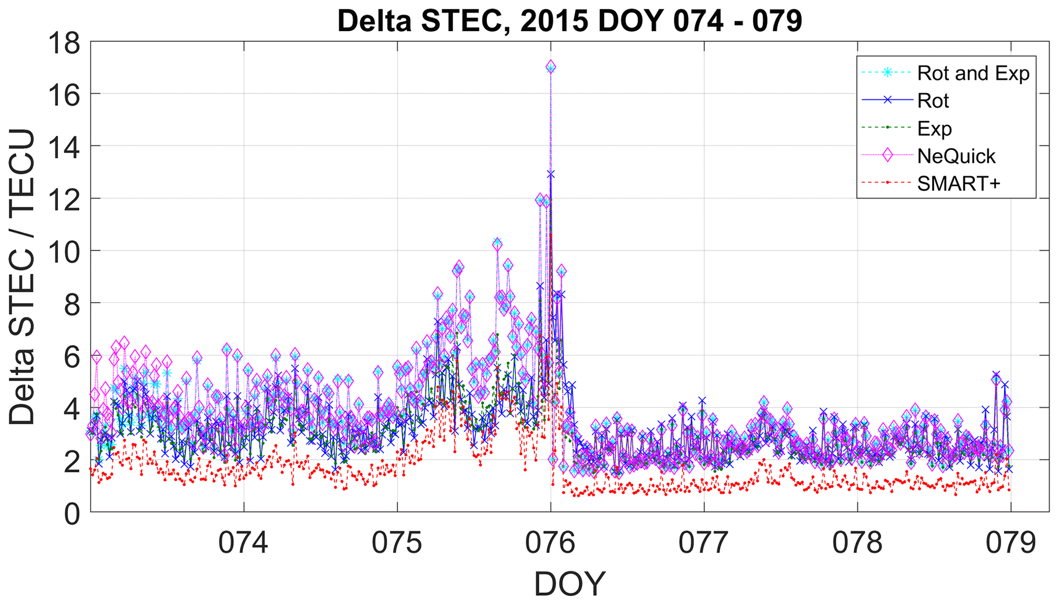
Figures 9 and 10 plot ΔSTEC values versus time for the selected periods. Noticeable is the increase in ΔSTEC during the storm on DOY 76. During the rest of the period, ΔSTEC is below 8 TECU. During both periods, SMART+ generates the lowest ΔSTEC values. ΔSTEC of the methods rotation and exponential decay are, in most of the cases, higher than SMART+ delta STEC values and lower than the NeQuick model. ΔSTEC of the method rotation with exponential decay is similar to the NeQuick model.
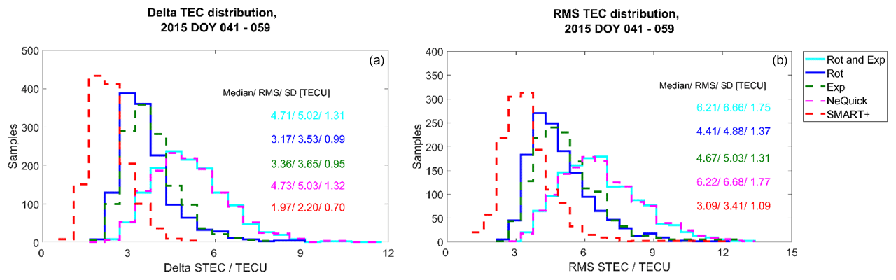
Figure 11Plausibility check for the quiet period. Distributions of the delta STEC (a) and RMS STEC (b) values.
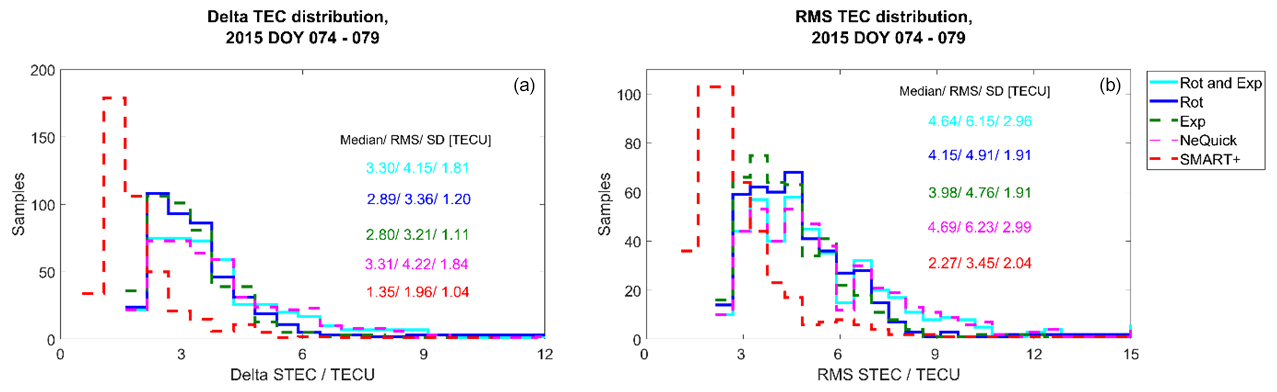
Figure 12Plausibility check for the perturbed period. Distributions of the delta STEC (a) and RMS STEC (b) values.
Figures 11 and 12 present the distribution of ΔSTEC and the RMS error (see Eq. 15) for the quiet and perturbed periods respectively. Figure 11 confirms the conclusions we have drawn so far from Figs. 8 and 9. SMART+ delivers the lowest ΔSTEC and RMS values, followed by the method rotation and then by the method exponential decay. Rotation with exponential decay performs similarly to the NeQuick model. For the perturbed period, SMART+ again delivers the lowest ΔSTEC and RMS statistics, followed by the exponential decay and the rotation, with similar results.
4.3 Validation with independent space-based STEC data
In order to validate the methods with respect to their capability to estimate independent STEC, the LEO satellites of Swarm A and GRACE have been used. The STEC measurements of these satellites are not assimilated by the tested methods.
For each of the three LEO satellites, the residuals between STECmeas and STECest are calculated and denoted as . Furthermore, the absolute values of the residuals are considered.
In general, for the quiet period, the STEC measurements of Swarm A vary below 105 TECU, and they are below 170 TECU for the second period. For the GRACE satellite, the STEC measurements are below 282 TECU for the quiet period and below 264 TECU for the second period.

Figure 13Histograms of the STEC residuals (a) and absolute residuals (b) during the quiet period for Swarm A.
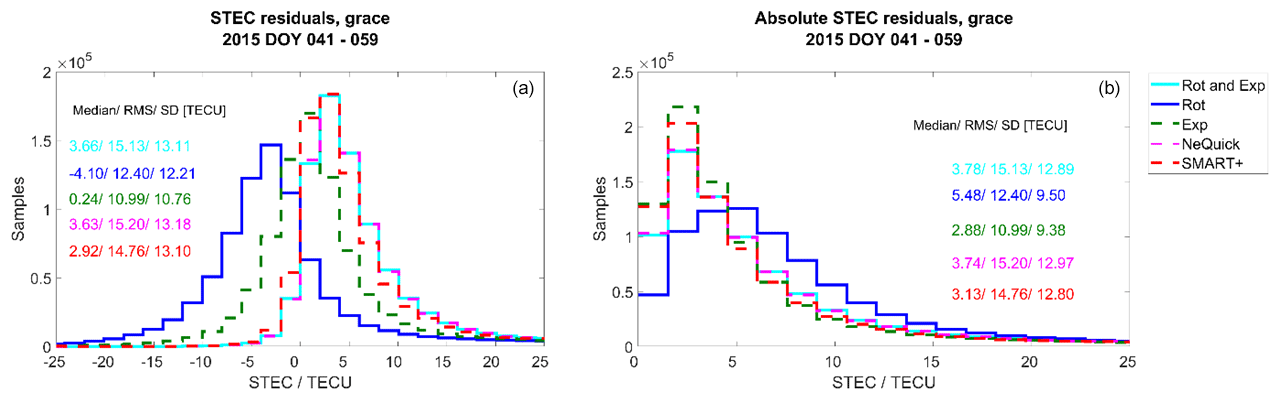
Figure 14Histograms of the STEC residuals (a) and absolute residuals (b) during the quiet period for GRACE.
Figures 13 and 14 display the histograms of the STEC residuals during the quiet period for Swarm A and GRACE respectively. Presented are the distributions of the residuals dTEC and the absolute residuals . Also plotted are the median, SD and RMS of the corresponding residuals. Figures 15 and 16 depict the histograms of the STEC residuals during the perturbed period.
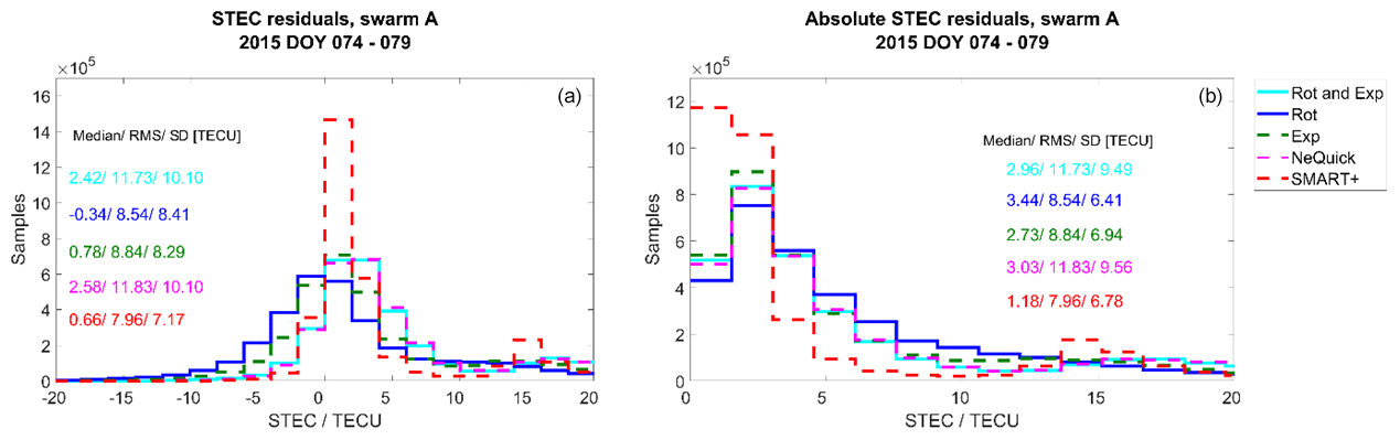
Figure 15Histograms of the STEC residuals (a) and absolute residuals (b) during the perturbed period for Swarm A.
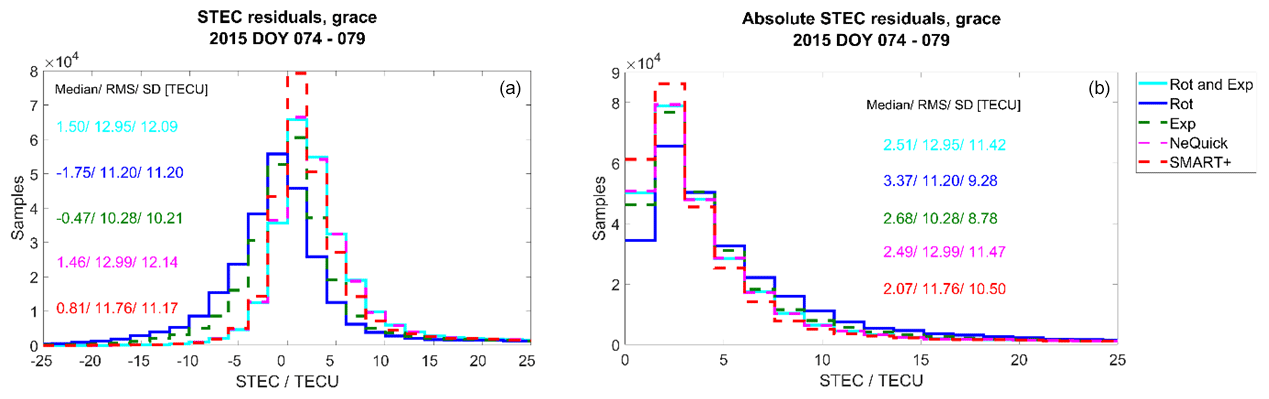
Figure 16Histograms of the STEC residuals (a) and absolute residuals (b) during the perturbed period for GRACE.
Again, the NeQuick model seems to underestimate the measured STEC during both periods for GRACE and Swarm A satellites. Compared to the NeQuick model, during both periods the methods of SMART+ and exponential decay decrease the residuals and the absolute residuals between measured and estimated STEC for both GRACE and Swarm A satellites. The method rotation with exponential decay performs, for both periods, very similarly to the NeQuick model. The performance of the method rotation is partly even worse than the one of the background model. Our impression is that the number and the distribution of the assimilated measurements is too small and the angle too limited to be sufficient to dispense with a background model, as is the case with the rotation method, which uses the model only for the estimation of the systematic error.
Regarding the STEC of Swarm A, the lowest residuals and the most reduction, in comparison to the NeQuick model, are achieved by SMART+. The median and the SD of the SMART+ residuals are ∼ 0.3 and ∼ 3.4 TECU respectively for the quiet period and ∼ 0.7 and ∼ 7 TECU for the perturbed period. Compared to the NeQuick model, the absolute median value is reduced by up to 64 % by SMART+ during the quiet period and by up to 61 % during the perturbed period. The SD value is decreased by up to 47 % during the quiet period and up to 29 % during the storm period. The second lowest residuals are achieved by the exponential decay; here, the median of the residuals is around 0.2 TECU for the quiet period and around 0.8 TECU for the perturbed period.
Regarding the STEC of GRACE during the quiet period, the lowest residuals and the most reduction in comparison to the background, are achieved by the exponential decay, followed by SMART+. Exponential decay reduces the background absolute median value by up to 26 % and the SD value by up to 28 %. The median of the residuals is around 0.2 TECU. For SMART+, the median of the residuals is around 2.9 TECU. During the perturbed period, SMART+ reduces the absolute median, at most, by 17 % and the SD by 9 %. The exponential decay does not reduce the absolute median, compared to NeQuick, but it reduces the absolute SD value by 23 %. The median of the residuals is around −0.5 TECU for exponential decay and around 0.8 TECU for SMART+.
Comparing the quiet and storm conditions, in general an increase in the RMS and SD of the Swarm A residuals is observable for the NeQuick model and all tomography methods regarding both satellites. This is not the case for the GRACE residuals.
4.4 Validation with independent LP in situ electron densities
In this section, we further extend our analyses to the validation of the methods with independent LP in situ electron densities of the three Swarm satellites. According to the locations of the LP measurements, the estimated electron density values are interpolated (by a 3D interpolation, using the MATLAB built-in function of scatteredInterpolant.m) from the 3D electron density reconstructions. For each satellite, the measured electron density Nemeas is compared to the estimated one Neest. In particular, we calculate the residuals , the absolute residuals |dNe|, the relative residuals and the absolute relative residuals .
Figure 17 depicts the distribution of the residuals dNe for the quiet period along with the median, SD and RMS values, with Fig. 17a, b and c each presenting one of the Swarm satellites. In Fig. 18, the histograms of and are given for the same period. In Fig. 18 we do not separate the values for the different satellites because these are similar. Figures 19 and 20 show the corresponding histograms for the perturbed period.

Figure 17Validation with LP data. Distribution of Swarm A, B and C (separated) electron density residuals for the quiet period.
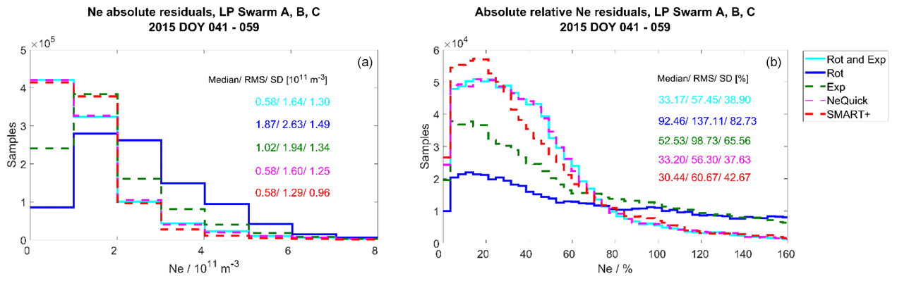
Figure 18Validation with LP data. Distribution of the Swarm absolute and absolute relative electron density residuals for the quiet period.
The electron densities of the NeQuick model are, in median, slightly higher than the LP in situ measurements for all three satellites during both periods. The median and SD values for the residuals produced by NeQuick are ∼ 33 % and ∼ 38 % respectively during the quiet period. For the perturbed period, we observe higher median and SD values of ∼ 45 % and ∼ 56 % respectively. The increase in the RMS and SD values of the absolute residuals is also visible for all the considered reconstruction methods.
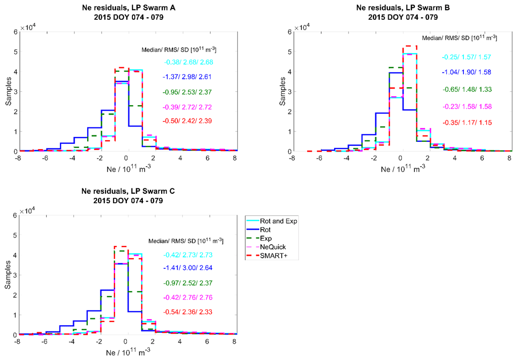
Figure 19Validation with LP data. Distribution of the Swarm A, B and C (separated) electron density residuals for the perturbed period.

Figure 20Validation with LP data. Distribution of the Swarm absolute and absolute relative electron density residuals for the perturbed period.
The methods of SMART+ and rotation with exponential decay follow the trend of the model and show similar distributions in Figs. 17 and 19. Comparing these two methods with the NeQuick model, the performance of SMART+ is slightly better, reducing the median of the absolute and absolute relative residuals by up to 8 %. Furthermore, during both periods, SMART+ reduces the SD values of the values by up to 23 %. However, the SD and RMS values of the residuals for SMART+ during the quiet period are higher than those of the NeQuick model. The median and SD values of the residuals for SMART+ are ∼ 30 % and ∼ 43 % respectively during the quiet period and higher during perturbed period, namely ∼ 43 % and ∼ 53 % respectively. The statistics of the methods exponential decay and rotation are worse than those of NeQuick.
In this paper, we assess three different propagation methods for an ensemble Kalman filter approach in the case that a physical propagation model is not available or is discarded due to the computational burden. We validate these methods with independent STEC observations of the satellites of GRACE and Swarm A and with independent Langmuir probes data of the three Swarm satellites. The methods are compared to the algebraic reconstruction method SMART+, which serves as a benchmark, and to the background model NeQuick for periods of the year 2015 covering quiet to perturbed ionospheric conditions.
Overlooking all the validation results, the methods of SMART+ and exponential decay reveal the best performance with the lowest residuals, whereas the method rotation with exponential decay provides only a small improvement compared to the NeQuick model. While SMART+ modifies the electron densities of the background model around the measurement geometry and produces rather small patches, the EnKF produces larger and smoother patterns. As expected, the validations indicate that the electron density estimates of the EnKF are not only dependent on the current measurement geometry but also on prior assimilations.
The plausibility check in Sect. 4.2 shows that all methods successfully reduce the STEC residuals and provide better results than the background model. SMART+ demonstrates the best performance, and lowers the error statistics of the NeQuick model by up to 86 %, followed by the method rotation, which decreases the median of the residuals by up to 83 %. The method exponential decay reduces the median by up to 55 %, but the SD values stay almost on the same level as for the NeQuick model.
Although the EnKF with the method rotation reproduces the assimilated STEC data well, less accurate estimates are obtained in the validation with independent data. We assume that this has two main reasons. First, as the only propagation method, rotation is not anchored by the background model. Second, the number of the assimilated measurements is low compared to the number of unknowns, and the available measurements are unevenly distributed and angle limited. Both together could lead to increased deviations in the estimates of the truth.
The methods SMART+ and the EnKF with exponential decay provide the best estimates of the independent STEC and reduce the STEC residuals by up to 64 % for Swarm A and 28 % for GRACE, compared to the NeQuick model. SMART+ generates the smallest residuals for the STEC measurements of Swarm A, and exponential decay performs the best for STEC measurements of GRACE.
Concerning the estimation of independent electron densities of the Langmuir probes, SMART+ shows the best results, reducing the absolute residuals by up to 23 %. The median and SD values of the absolute residuals for SMART+ are ∼ 30 % and ∼ 43 % respectively during quiet ionospheric conditions and ∼ 43 % and ∼ 53 % respectively during perturbed ionospheric conditions. The distributions of the residuals produced by rotation with exponential decay are similar to the ones of the NeQuick model. In general, all the considered methods generate relatively high residuals. These observations could be explained by the fact that the independent electron density measurements are located at the lower edge of the reconstructed area, and all the assimilated measurements are located above. Additionally, Swarm LPs were found to underestimate the true electron density systematically (see Sect. 3.3.2). In order to obtain better results for the lower altitudes, it might, therefore, be necessary to apply a kind of anchor point for the lower altitudes within the reconstruction procedure which could, for instance, be the Swarm LPs electron density measurements themselves.
Another approach for improving the reconstructions could be to precondition the background model, for example, in terms of F2 layer characteristics or the plasmapause location (see, for example, Bidaine and Warnant, 2010; Gerzen et al., 2017).
To obtain a comprehensive final impression of the performance of the investigated methods and to gain insight into the ability of the methods to correctly characterize the shapes of the electron density profiles, we intend to continue the validation of the methods with additional, independent measurements of the plasmasphere and topside ionosphere, for example, coherent scatter radar data.
The data that were used can be found in Sect. 3.3 or are available upon request.
TG contributed the main ideas to the methods presented in this article, implemented the EKF, carried out the validation and wrote most of the sections. DM helped to fine-tune the propagation methods, took care of the operation of the background model and contributed sections to the final article. All co-authors helped to interpret the results, read and comment on the article.
The authors declare that they have no conflict of interest.
We thank NOAA (ftp://ftp.ngdc.noaa.gov/STP/GEOMAGNETIC_DATA/INDICES/, last access: 2 November 2020) and the World Data Center Kyoto (http://wdc.kugi.kyoto-u.ac.jp/dstdir/index.html, last access: 2 November 2020) for making the geo-related data, F10.7, Kp and DST indices available. We are grateful to the European Space Agency for providing the Swarm data (https://swarm-diss.eo.esa.int/, last access: 2 November 2020) and to the COSMIC Data Analysis and Archive Center (CDAAC) for providing the STEC data of several LEO satellites (http://cdaac-www.cosmic.ucar.edu/cdaac/tar/rest.html, last access: 2 November 2020). Additionally, we express our gratitude to the Aeronomy and Radiopropagation Laboratory of the Abdus Salam International Centre for Theoretical Physics Trieste, Italy, for providing the NeQuick (version 2.0.2) for scientific purposes.
This study was performed as part of the MuSE project (grant no. 273481272) and funded by the DFG as a part of the Priority Programme of DynamicEarth (grant no. SPP-1788).
This paper was edited by Steve Milan and reviewed by two anonymous referees.
Angling, M. J.: First assimilation of COSMIC radio occultation data into the Electron Density Assimilative Model (EDAM), Ann. Geophys., 26, 353–359, 2008.
Angling, M. J. and Cannon, P. S.: Assimilation of radio occultation measurements into background ionospheric models, Radio Sci., 39, RS1S08, https://doi.org/10.1029/2002RS002819, 2004.
Banville, S.: Improved convergence for GNSS precise point positioning, Ph.D. dissertation, Department of Geodesy and Geomatics Engineering, Technical Report No. 294, University of New Brunswick, Fredericton, New Brunswick, Canada, available at: https://unbscholar.lib.unb.ca/islandora/object/unbscholar:6500 (last access: 2 November 2020) 2014.
Bidaine B. and R. Warnant: Assessment of the NeQuick model at mid-latitudes using GNSS TEC and ionosonde data, Adv. Space Res., 45, 1122–1128, 2010.
Bilitza, D., McKinnell, L.-A., Reinisch, B., and Fuller-Rowell, T.: The International Reference Ionosphere (IRI) today and in the future, J. Geodesy, 85, 909–920, https://doi.org/10.1007/s00190-010-0427-x, 2011.
Bust, G. S. and Mitchell, C. N.: History, current state, and future directions of ionospheric imaging, Rev. Geophys., 46, RG1003, https://doi.org/10.1029/2006RG000212, 2008.
Chen, P. and Yao, Y.: Research on global plasmaspheric electron content by using LEO occultation and GPS data, Adv. Space Res., 55, 2248–2255, https://doi.org/10.1016/j.asr.2015.02.004, 2015.
Codrescu, S. M., Codrescu, M. V., and Fedrizzi, M.: An Ensemble Kalman Filter for the thermosphere-ionosphere, Space Weather, 16, 57–68, https://doi.org/10.1002/2017SW001752, 2018.
Dettmering, D.: Die Nutzung des GPS zur dreidimensionalen Ionosphärenmodellierung. PhD Thesis, University of Stuttgart, available at: http://elib.uni-stuttgart.de/opus/volltexte/2003/1411/ (last access: 2 November 2020), 2003.
Elvidge, S. and Angling, M. J.: Using the local ensemble Transform Kalman Filter for upper atmospheric modelling, J. Space Weather Space Clim., 9, 1–12, https://doi.org/10.1051/swsc/2019018, 2019.
Evensen, G.: Sequential data assimilation with a nonlinear quasi-geostrophic model using Monte Carlo methods to forecast error statistics, J. Geophys. Res., 99, 10143–10162, https://doi.org/10.1029/94JC00572, 1994.
Evensen, G.: The Ensemble Kalman Filter: theoretical formulationand practical implementation, Ocean Dynam., 53, 343–367, https://doi.org/10.1007/s10236-003-0036-9, 2003.
Gerzen, T. and Minkwitz, D.: Simultaneous multiplicative column normalized method (SMART) for the 3D ionosphere tomography in comparison with other algebraic methods, Ann. Geophys., 34, 97–115, https://doi.org/10.5194/angeo-34-97-2016, 2016.
Gerzen, T., Minkwitz, D., and Schlueter, S.: Comparing different assimilation techniques for the ionospheric F2 layer reconstruction, J. Geophys. Res.-Space, 120, 6901–6913, https://doi.org/10.1002/2015JA021067, 2015.
Gerzen, T., Wilken, V., Minkwitz, D., Hoque, M., and Schlüter, S.: Three-dimensional data assimilation for ionospheric reference scenarios, Ann. Geophys., 35, 203–215, https://doi.org/10.5194/angeo-35-203-2017, 2017.
Heise, S., Jakowski, N., Wehrenpfennig, A., Reigber, C., and Lühr, H.: Sounding of the topside ionosphere/plasmasphere based on GPS measurements from CHAMP: Initial results, Geophys. Res. Lett., 29, 44-1–44-4, https://doi.org/10.1029/2002GL014738, 2002.
Hernandez-Pajares, M., Juan, J. M., and Sanz, J.: New approaches in global ionospheric determination using ground GPS data, J. Atmos. Sol.-Terr. Phys., 61, 1237–1247, 1999.
Hochegger, G., Nava, B., Radicella, S. M., and Leitinger, R.: A Family of Ionospheric Models for Different Uses, Phys. Chem. Earth Pt. C, 25, 307–310, https://doi.org/10.1016/S1464-1917(00)00022-2, 2000.
Howe, B. and Runciman, K.: Tomography of the ionosphere: Four-dimensional simulations, Radio Sci., 33, 9–128, 1998.
Howe, B. M., Runciman, K., and Secan, J. A.: Tomography of the ionosphere: Four-dimensional simulations, Radio Sci., 33, 109–128, 1998.
Kalnay, E.: Atmospheric Modeling, Data Assimilation and Predictability, Cambridge University Press, Cambridge, UK, 140–141, 2011.
Klimenko, M. V., Klimenko, V. V., Zakharenkova, I. E., and Cherniak, I. V.: The global morphology of the plasmaspheric electron content during Northern winter 2009 based on GPS/COSMIC observation and GSM TIP model results, Adv. Space Res., 55, 2077–2085, https://doi.org/10.1016/j.asr.2014.06.027, 2015.
Lee, I. T., Matsuo, T., Richmond, A. D., Liu, J. Y., Wang, W., Lin, C. H., Anderson, J. L., and Chen, M. Q.: Assimilation of FORMOSAT-3/COSMIC electron density profiles into a coupled thermosphere/ionosphere model using ensemble Kalman filtering, J. Geophys. Res., 117, A10318, https://doi.org/10.1029/2012JA017700, 2012.
Liang, W., Limberger, M., Schmidt, M., Dettmering, D., Hugentobler, U., Bilitza, D., Jakowski, N., Hoque, M. M., Wilken, V., and Gerzen, T.: Regional modeling of ionospheric peak parameters using GNSS data – an update for IRI, Adv. Space Res., 55, 1981–1993, https://doi.org/10.1016/j.asr.2014.12.006, 2015.
Liang, W., Limberger, M., Schmidt, M., Dettmering, D., and Hugentobler, U.: Combination of ground- and space-based GPS data for the determination of a multi-scale regional 4-D ionosphere model, in: IAG 150 Years, IAG Symposia, edited by: Rizos, C. and Willis, P., 143, 751–758, https://doi.org/10.1007/1345_2015_25, 2016.
Lomidze, L., Scherliess, L., and Schunk, R. W.: Magnetic meridional winds in the thermosphere obtained from Global Assimilation of Ionospheric Measurements (GAIM) model, J. Geophys. Res.-Space, 120, 8025–8044, https://doi.org/10.1002/2015JA021098, 2015.
Lomidze, L., Knudsen, D. J., Burchill, J., Kouznetsov, A., and Buchert, S. C.: Calibration and validation of Swarm plasma densities and electron temperatures using ground-based radars and satellite radio occultation measurements, Radio Sci., 53, 15–36, https://doi.org/10.1002/2017RS006415, 2018.
Minkwitz, D., van den Boogaart, K. G., Gerzen, T., and Hoque, M. M.: Tomography of the ionospheric electron density with geostatistical inversion, Ann. Geophys., 33, 1071–1079, https://doi.org/10.5194/angeo-33-1071-2015, 2015.
Minkwitz, D., van den Boogaart, K. G., Gerzen, T., Hoque, M., and Hernández-Pajares, M.: Ionospheric tomography by gradient enhanced kriging with STEC measurements and ionosonde characteristics, Ann. Geophys., 34, 999–1010, https://doi.org/10.5194/angeo-34-999-2016, 2016.
Nava, B., Coisson, P., and Radicella, S. M.: A new version of the NeQuick ionosphere electron density model, J. Atmos. Sol.-Terr. Phy., 70, 1856–1862, https://doi.org/10.1016/j.jastp.2008.01.015, 2008.
Nikoukar, R., Bust, G., and Murr, D.: Anovel data assimilation technique for the plasmasphere, J. Geophhys. Res.-Space Phys., 120, 8470–8485, https://doi.org/10.1002/2015JA021455, 2015.
Odijk, D.: Precise GPS positioning in the presence of ionospheric delays. Publications on geodesy, Vol. 52, The Netherlands Geodetic Commission, Delft, ISBN-13: 978 90 6132 278 8, 2002.
Olivares-Pulido, G., Terkildsen, M., Arsov, K., Teunissen, P. J. G., Khodabandeh, A., and Janssen, V.: A 4D tomographic ionospheric model to support PPP-RTK, J. Geodesy, 93, 1673–1683, https://doi.org/10.1007/s00190-019-01276-4, 2019.
Radicella, S. M. and Leitinger, R.: The evolution of the DGR approach to model electron density profiles, Adv. Space. Res., 27, 35–40, https://doi.org/10.1016/S0273-1177(00)00138-1, 2001.
Schaer, S.: Mapping and predicting the Earth's ionosphere using the global positioning system, Ph.D. dissertation, Astron Institute, University of Bern, Berne, available at: http://ftp.aiub.unibe.ch/papers/ionodiss.pdf (last access: 2 November 2020), 1999.
Scherliess, L., Thompson, D. C., and Schunk, R. W.: Ionospheric dynamics and drivers obtained from a physicsbased data assimilation model, Radio Sci., 44, RS0A32, https://doi.org/10.1029/2008RS004068, 2009.
Schmidt, M., Bilitza, D., Shum, C., and Zeilhofer, C.: Regional 4-D modelling of the ionospheric electron density, Adv. Space Res., 42, 782790, https://doi.org/10.1016/j.asr.2007.02.050, 2008.
Schmidt, M., Dettmering, D., and Seitz, F.: Using B-spline expansions for ionosphere modeling, in: Handbook of Geomathematics, edited by: Freeden, W., Nashed, M. Z., and Sonar, T., 2nd Edn., Springer, 939–983, https://doi.org/10.1007/978-3-642-54551-1_80, 2015.
Schunk, R. W., Scherliess, L., Sojka, J. J., Thompson, D. C., Anderson, D. N., Codrescu, M., Minter, C., Fuller-Rowell, T. J., Heelis, R. A., Hairston, M., and Howe, B. M.: Global Assimilation of Ionospheric Measurements (GAIM), Radio Sci., 39, RS1S02, https://doi.org/10.1029/2002RS002794, 2004.
Schunk, R. W., Scherliess, L., Eccles, V., Gardner, L. C., Sojka, J. J., Zhu, L., Pi, X., Mannucci, A. J., Butala, M., Wilson, B. D., Komjathy, A., Wang, C., and Rosen, G.: Space weather forecasting with a Multimodel Ensemble Prediction System (MEPS), Radio Sci., 51, 1157–1165, https://doi.org/10.1002/2015RS005888, 2016.
Spencer, P. S. J. and Mitchell, C. N.: Imaging of 3-D plasmaspheric electron density using GPS to LEO satellite differential phase observations, Radio Sci., 46, RS0D04, https://doi.org/10.1029/2010RS004565, 2011.
Wang, C., Hajj, G., Pi, X., Rosen, I. G., and Wilson, B.: Development of the Global Assimilative Ionospheric Model, Radio Sci., 39, RS1S06, https://doi.org/10.1029/2002RS002854, 2004.
Wen, D., Yuan, Y., Ou, J., Huo, X., and Zhang, K.: Three-dimensional ionospheric tomography by an improved algebraic reconstruction technique, GPS Solut., 11, 251–258, https://doi.org/10.1007/s10291-007-0055-y, 2007.
Wen, D., Mei, D., and Du, Y.: Adaptive Smoothness Constraint Ionospheric Tomography Algorithm, Sensors, 20, 2404, https://doi.org/10.3390/s20082404, 2020.
Zeilhofer, C.: Multi-dimensional B-spline Modeling of Spatio-temporal Ionospheric Signals: DGK, Verlag der Bayerischen Akademie der Wissenschaften, Serie A, No. 123, ISBN: 3769682033, Munich, available at: https://dgk.badw.de/fileadmin/user_upload/Files/DGK/docs/a-123.pdf (last access: 2 November 2020), 2008.
Zeilhofer, C., Schmidt, M., Bilitza, D., and Shum, C. K.: Regional 4-D modeling of the ionospheric electron density from satellite data and IRI, Adv. Space Res., 43, 1669–1675, 2009.