A numerical method to improve the spatial interpolation of water vapor from numerical weather models: a case study in South and Central America

Commonly, numerical weather model (NWM) users can get the vertically integrated water vapor (IWV) value at a given location from the values at nearby grid points. In this study we used a validated and freely available global navigation satellite system (GNSS) IWV data set to analyze the very well-known effect of height differences. To this end, we studied the behavior of 67 GNSS stations in Central and South America with the prerequisite that they have a minimum of 5 years of data during the period from 2007 to 2013. The values of IWV from GNSS were compared with the respective values from ERA-Interim and MERRA-2 from the same period. Firstly, the total set of stations was compared in order to detect cases in which the geopotential difference between GNSS and NWM required correction. An additive integral correction to the IWV values from ERA-Interim was then proposed. For the calculation of this correction, the multilevel values of specific humidity and temperature given at 37 pressure levels by ERA-Interim were used. The performance of the numerical integration method was tested by accurately reproducing the IWV values at every individual grid point surrounding each of the GNSS sites under study. Finally, considering the IWV_GNSS values as a reference, the improvement introduced to the IWV_ERA-Interim values after correction was analyzed. In general, the corrections were always recommended, but they are not advisable in marine coastal areas or on islands as at least two grid points of the model are usually in the water. In such cases, the additive correction could overestimate the IWV.

1 Introduction

Water vapor is an abundant natural greenhouse gas in the atmosphere. The knowledge of its variability in time and space is very important with respect to understanding the global climate system (Dessler et al., 2008). Most of the regional comparisons of IWV from the global navigation satellite system (GNSS) are aimed at validating the technique via comparison with radiosonde and microwave radiometers where available. An example of this is the work of Van Malderen et al. (2014), who compared IWV GPS (Global Positioning System) information with IWV derived from ground-based sun photometers, radiosondes and satellite-based values from GOME, SCIAMACHY, GOME-2 and AIRS instruments at 28 sites in the Northern Hemisphere. Because their comparison is oriented toward a climatology application, they deal with long-term time series (>10 years). The authors asseverate that the mean biases of the GPS with the different instruments only vary between −0.3 and 0.5 kg m⁻², but there are large standard deviations especially for the satellite instruments.

However, some other comparisons examine the IWV_GNSS values with respect to the respective estimates from numerical weather models (NWMs). If focusing on the application of the current state-of-the-art ERA-Interim reanalysis from the European Centre for Medium-Range Weather Forecasts (ECMWF), both on a local and global scale, some recent papers deserve to be mentioned. For example, Heise et al. (2009) used ground pressure data from ECMWF to calculate IWV from 5 min zenith total delay (ZTD) at stations where meteorological data are not available. The authors validated their results using stations with local measurements of pressure and temperature. They also compared IWV from GPS with respect to IWV from ERA-Interim on a global scale. The authors found that IWV from GPS and ECMWF show good agreement at most stations on the global scale, except in mountain regions. Moreover, they addressed the fact that temporal station pressure interpolation may result in up to 0.5 kg m⁻² IWV uncertainty if a local weather event occurred. According to the authors, this phenomenon is particularly noticeable in the tropics and is due to the fact that the ECMWF analysis does not adequately represent the local situation if faced with an increase in the diurnal cycle of the surface atmospheric pressure.

Buehler et al. (2012) compared IWV values over Kiruna in the north of Sweden from five different techniques (radiosondes, GPS, a ground-based Fourier transform infrared (FTIR) spectrometer, a ground-based microwave radiometer and a satellite-based microwave radiometer) with IWV from ERA-Interim reanalysis. The processed GPS data set covered a 10-year period from November 1996 to November 2006. The authors found good overall agreement between IWV from GPS and from ERA-Interim, with mean differences of 0.29 kg m⁻² and a standard deviation 1.25 kg m⁻². They also point out that ERA-Interim is drier than the GPS at small IWV values and slightly moister at high IWV values (above 15 kg m⁻²). The authors also considered altitude limits when comparing measurements from different data sets. They proposed an empirical solution by computing linear regression slopes as a function of height and corrected all measurements to a common reference altitude of 430 m. Thus, they established a relative bias of −3.5 % per 100 m that introduced absolute errors below 0.2 kg m⁻². Nevertheless, they asseverated that the good performance of the method depends on location and probably on season.

Ning et al. (2013) evaluated IWV from GPS in comparison with IWV from ERA-Interim and IWV from the regional Rossby Centre atmospheric (RCA) climate model at 99 European sites for a 14-year period. Because RCA is not an assimilation model, the standard deviation of RCA − GPS was 3 times larger than ERA-GPS. The IWV difference for individual sites varies from −0.21 to 1.12 kg m⁻² for ERA-GPS and the corresponding standard deviation is 0.35 kg m⁻². The authors investigated the influence of the differences between NWM and GPS in the vertical and horizontal positions. In particular, they studied subsets of stations with absolute height difference values smaller than 100 m. Consequently, they did not consider if there were over- or underestimations by the models. Thus, they found monthly mean IWV difference values smaller than 0.5 kg m⁻². Moreover, the authors also highlighted that the models overestimated IWV for sites near the sea.

Bordi et al. (2014) studied global trend patterns of the yearly mean of IWV from the 20th century atmosphere model (ERA-20CM) and ERA-Interim, which are both from ECMWF. The authors highlighted a regional dipole pattern of interannual climate variability over South America from ERA-Interim data. According to this study, the Andean Amazon Basin and northeast Brazil are characterized by rising and decreasing water content associated with water vapor convergence (divergence) and upward (downward) mass fluxes, respectively. In addition, the authors also compared IWV from ERA-Interim with the values estimated at two GPS stations in Bogotá and Brasilia. Such comparison on a monthly timescale uncovered a systematic bias attributed to a lack of coincidence in the elevation of the GPS stations and the model grid points.

Mengistu Tsidu et al. (2015) presented a comparison between IWV from a Fourier transform infrared spectrometer (FTIR, at Addis Ababa), GPS, radiosondes and ERA-Interim over Ethiopia for the period from 2007 to 2011. The study is focused on the characterization of the different error sources affecting the data time series. In particular, from the study of diurnal and seasonal variabilities, the authors addressed differences in the magnitude and sign of the IWV bias between ERA-Interim and GPS. They linked this effect to the sensitivity of the convection model with respect to the topography.

Wang et al. (2015) performed a 12-year comparison of IWV from three third-generation atmospheric reanalysis models including ERA-Interim, MERRA and the Climate Forecast System Reanalysis (CFSR) on a global scale. IWV values from the reanalysis models were also compared with radiosonde observations on land and remote sensing systems (RSS) on satellites over oceans. The authors asseverated that the main discrepancies between the three data sets are in central Africa, northern South America and in highland areas.

In this paper, we investigated the differences between IWV from GNSS using data products from Bianchi et al. (2016a) and IWV values given by ERA-Interim and MERRA-2. The comparison was performed by considering the geopotential differences (Δz) between each GNSS station and the corresponding values assigned by the models. We proposed an additive numerical correction to the IWV from the NWM, and the strategy was tested for the ERA-Interim reanalysis model. Section 2 describes the different sets of data used in this study. In the following, we give an explanation of the methodology and present the results obtained after applying the proposed correction to the IWV values from ERA-Interim.

2 Data

2.1 IWV from GNSS

GNSS data are the main source of information for the spatial and temporal distribution of water vapor. Thus, the main variable considered is the IWV estimated from the delay caused by the troposphere to the GNSS radio signals during its travel from the satellite to the ground receiver. The total delay projected onto the zenith direction (ZTD) is usually split into two contributions: the hydrostatic delay (ZHD – zenith hydrostatic delay), depending merely on the atmospheric pressure, and the zenith wet delay (ZWD), depending mainly on the humidity. The IWV_GNSS can be obtained from the ZWD by multiplying it by a function of the mean temperature of the atmosphere.

The reference database of IWV_GNSS used in this study comes from the geodetic processing of over 136 tracking stations on the American continent, located from southern California to Antarctica (see Fig. 1), during a 7-year period from January 2007 to December 2013 (Bianchi et al., 2016b). Specifically, the data series of IWV_GNSS used here is restricted to the 67 stations with IWV time series spanning more than 5 years (see Fig. 1 and Table 1). More details regarding the steps, models and conventions followed by the geodetic processing to obtain the IWV_GNSS values are given in Bianchi et al. (2016a).

Table 1 Geopotential values at the selected GNSS stations. Values of z_ERA-Interim and z_MERRA-2 come from a bilinear interpolation of the four gridded values of z around the GNSS site.

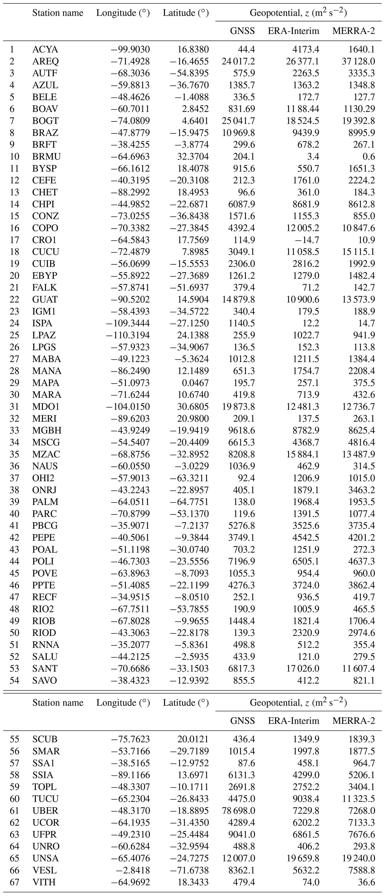
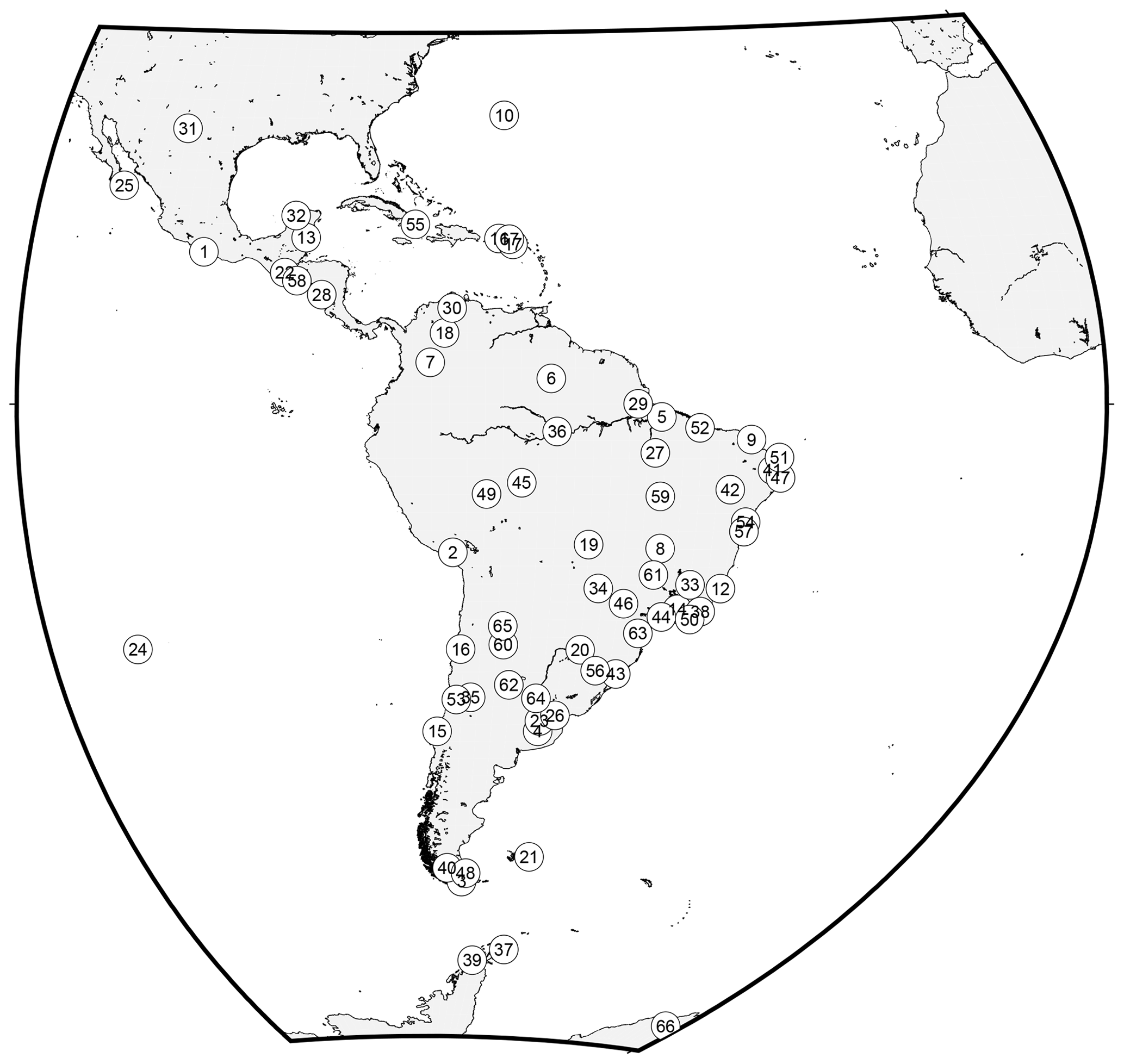
Figure 1 Location of the GNSS stations (see Tables 1 and 2).

2.2 IWV from NWM

The values of columnar integrated content of water vapor (IWV) as reanalysis products from ERA-Interim (Dee et al., 2011) and MERRA-2 (GMAO, 2015; Bosilovich et al., 2015; Gelaro et al., 2017) were evaluated in this study. The horizontal resolutions are 0.25^∘ × 0.25^∘ for ERA-Interim and 0.625^∘ × 0.50^∘ for MERRA-2. Because ERA-Interim data are given four times a day, in order to perform the comparison (even if MERRA-2 gives hourly data), we collected IWV data from MERRA-2 every 6 h at 00:00, 06:00, 12:00 and 18:00 UT (universal time). Thus, in order to be able to carry out the comparison, MERRA-2 was only partially evaluated.

ERA-Interim is the global atmospheric reanalysis produced by the European Centre for Medium-Range Weather Forecasts (ECMWF). It covers the period from 1979 to present and supersedes the ERA-40 reanalysis. ERA-Interim addresses some of the difficulties of ERA-40 with respect to data assimilation mainly regarding the representation of the hydrological cycle, the quality of the stratospheric circulation and the consistency in terms of reanalyzed geophysical fields (Dee et al., 2011).

MERRA-2 is the successor of the Modern-Era Retrospective Analysis for Research and Applications (MERRA) from NASA's Global Modeling and Assimilation Office (Rienecker et al., 2011). MERRA-2 is improved because it contains fewer trends and jumps linked to changes in the observing systems than MERRA. Additionally, MERRA-2 assimilates observations not available to MERRA and reduces bias and imbalances in the water cycle (Gelaro et al., 2017). Moreover, the longitudinal resolution of MERRA-2 data is changed from 0.667^∘ in MERRA to 0.625^∘, whereas the latitudinal resolution remains unchanged (0.5^∘) (Bosilovich et al., 2015).

For this application, we used two different kind of data sets: 2-D values of the IWV from both reanalysis models along with the correspondent geopotential invariant; and three 3-D data sets from ERA-Interim, including the air temperature (T), the specific humidity (q) and the geopotential (z). These variables are given at 37 levels of atmospheric pressure from 1 to 1000 hPa.

We will use the terms z_i, T_i, p_i and q_i to refer to the value of the abovementioned variables at a given level “i” and at a given instant. This set of data will be used for the calculation of the integral correction that will be developed in the following section.

3 Methodology

As previously mentioned, even when both reanalysis models give grid values of the vertical integral of the water vapor, the solution provided by each model is linked to its respective geopotential surface invariant. Nevertheless, elevation differences between the geopotential from each model grid and that computed from the GNSS height must be addressed.

In order to compute the geopotential of the GNSS stations (z_GNSS) we followed the van Dam et al. (2010) algorithm. Because the geodetic coordinates ($\mathit{\varphi },\mathit{\lambda },h$) of the GNSS site are known, we obtained the orthometric height (H) at each GNSS station by correcting the ellipsoidal height using the EGM08 model (Pavlis et al., 2012). Thus, the geopotential is (van Dam et al., 2010)

$$\begin{array}{}\text{(1)}& z_{\mathrm{GNSS}}={\displaystyle \frac{g_s\left(\mathit{\varphi }\right)C\left(\mathit{\varphi }\right)H}{\left(C\right(\mathit{\varphi })+H)}},\end{array}$$

where the radius of the ellipsoid at geodetic latitude ϕ is

$$\begin{array}{}\text{(2)}& C\left(\mathit{\varphi }\right)={\left({\displaystyle \frac{{\cos }^{\mathrm{2}}\left(\mathit{\varphi }\right)}{a^{\mathrm{2}}}}+{\displaystyle \frac{{\sin }^{\mathrm{2}}\left(\mathit{\varphi }\right)}{b^{\mathrm{2}}}}\right)}^{-\mathrm{1}/\mathrm{2}}.\end{array}$$

Here a = 6 378 137 m and b = 6 356 752.3142 m are the semi-major and semi-minor axis of the WGS84 ellipsoid, respectively (Hofmann-Wellenhof and Moritz, 2006). Moreover, the value of the gravity on the ellipsoid at geodetic latitude ϕ can be written as follows (van Dam et al., 2010):

$$\begin{array}{}\text{(3)}& g_s\left(\mathit{\varphi }\right)=g_{\mathrm{E}}{\displaystyle \frac{\mathrm{1}+k_s{\sin }^{\mathrm{2}}\left(\mathit{\varphi }\right)}{\sqrt{\mathrm{1}-e^{\mathrm{2}}{\sin }^{\mathrm{2}}\left(\mathit{\varphi }\right)}}},\end{array}$$

where e²=0.00669437999014 is the first eccentricity squared of the WGS84 ellipsoid, g_E=9.7803253359 m s⁻² is the normal gravity at the Equator (Hofmann-Wellenhof and Moritz, 2006) and k_s=0.001931853 (van Dam et al., 2010).

For a given GNSS station, the respective geopotential from each of the two reanalysis models resulted from a bilinear interpolation of the respective invariant static geopotential at the four grid points around the GNSS site, referred to as $z_{\mathrm{NWM}}^k$ ($k=\mathrm{1},\mathrm{2},\mathrm{3},\mathrm{4}$). Because the points of the NWM grid surrounding the GNSS station have different geopotential values and those values are in turn different from z_GNSS, we propose to correct on each of these four points. Thus, if Δz^k refers to the difference between z_GNSS and $z_{\mathrm{NWM}}^k$,

$$\begin{array}{}\text{(4)}& \mathrm{\Delta }{z}^k=z_{\mathrm{GNSS}}-z_{\mathrm{NWM}}^k,k=\mathrm{1},\mathrm{2},\mathrm{3},\mathrm{4},\end{array}$$

where NWM corresponds to ERA-Interim or MERRA-2.

We will then propose a correction procedure that, by compensating for Δz^k in each of the four grid points, corrects the values of IWV_NWM. After “moving” the grid points to z_GNSS, a bilinear interpolation is performed to obtained the corrected value of IWV at the location of the GNSS site. In brief, this procedure is equivalent to lifting (or dropping, as appropriate) each of the grid points in order to create a plane at z_GNSS.

Prior to the correction, we analyze the performance of ERA-Interim and MERRA-2 with respect to GNSS. Thus, although IWV_GNSS is produced every 30 min and IWV_MERRA-2 is available hourly, we only consider the epochs when ERA-Interim data are available to perform the comparison at 00:00, 06:00, 12:00 and 18:00 UT. Table 2 shows the mean values of IWV from GNSS (${\stackrel{\mathrm{‾}}{\mathrm{IWV}}}_{\mathrm{GNSS}}$) during the period from 2007 to 2013 and its standard deviation for all of the stations. We assume that the static geopotential from the NWM at each GNSS site (z_NWM) is obtained from a bilinear interpolation of the static geopotential at the four grid points surrounding it ($z_{\mathrm{NWM}}^k$). Thus, Table 2 shows the geopotential difference ($\mathrm{\Delta }z=z_{\mathrm{GNSS}}-z_{\mathrm{NWM}}$) in addition to the respective differences of the mean values ($\mathrm{\Delta }\stackrel{\mathrm{‾}}{\mathrm{IWV}}={\stackrel{\mathrm{‾}}{\mathrm{IWV}}}_{\mathrm{GNSS}}-{\stackrel{\mathrm{‾}}{\mathrm{IWV}}}_{\mathrm{NWM}}$), where NWM indicates ERA-Interim and MERRA-2. All the averages are computed over the period from 2007 to 2013.

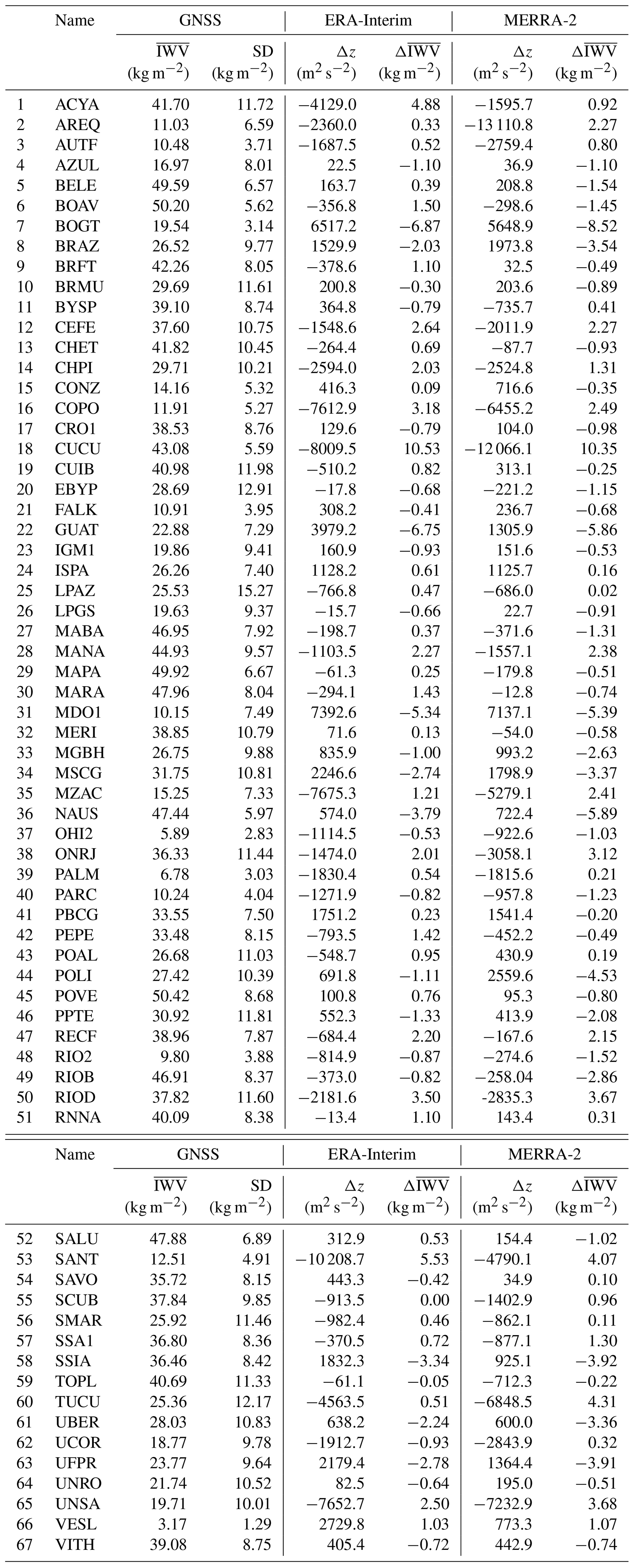
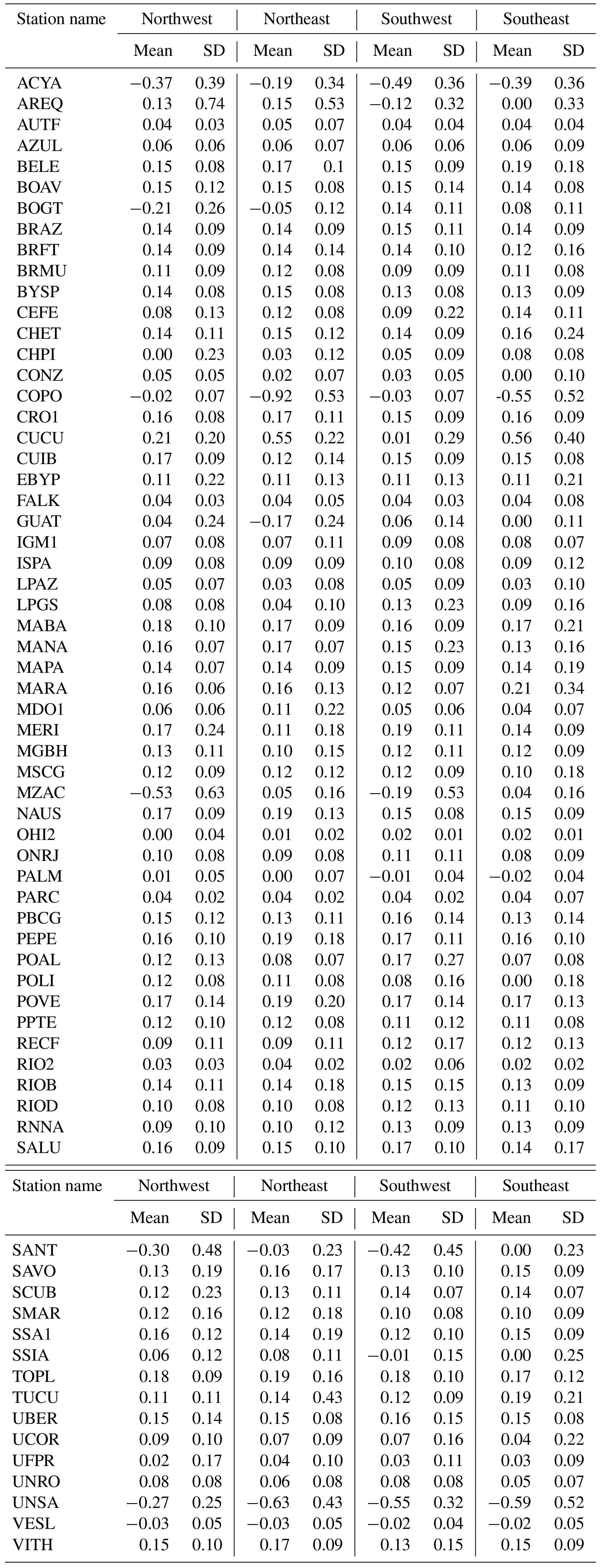
Table 2 Differences of the mean values of IWV ($\mathrm{\Delta }\stackrel{\mathrm{‾}}{\mathrm{IWV}}$) between GNSS and the NWM for the period from 2007 to 2013 at 67 stations located in South and Central America. The mean value ($\stackrel{\mathrm{‾}}{\mathrm{IWV}}$) from GNSS at each site is also given, and SD refers to the standard deviation. $\mathrm{\Delta }z=z_{\mathrm{GNSS}}-z_{\mathrm{NWM}}$ refers to the difference in the geopotential at each GNSS station.

In general, regarding Table 2, we can observe that the best agreements between the average IWV values from GNSS and the corresponding average from the models are where the Δz are small (e.g., CONZ, VITH, SMAR, LPGS, MAPA and SCUB, among others). In other words, the NWMs generally represent the IWV values very well ($\mathrm{\Delta }\stackrel{\mathrm{‾}}{\mathrm{IWV}}<\mathrm{1.5}$ kg m⁻²) if |Δz| is small. That means, the geopotential difference is in the order of 500 m² s⁻² at most.

Conversely, the difference of the model representation of the IWV with respect to GNSS increases as the height differences (Δz) become larger, and this is true for all values of ${\stackrel{\mathrm{‾}}{\mathrm{IWV}}}_{\mathrm{GNSS}}$. The SANT (${\stackrel{\mathrm{‾}}{\mathrm{IWV}}}_{\mathrm{GNSS}}\sim \mathrm{12}$ kg m⁻², |Δz|>10000 m² s⁻²) and CUCU (${\stackrel{\mathrm{‾}}{\mathrm{IWV}}}_{\mathrm{GNSS}}\sim \mathrm{43}$ kg m⁻², |Δz|∼8000 m² s⁻²) cases are good examples of this.

However, other than the abovementioned cases, which can be considered to be critical, the differences are also important at sites with moderate |Δz| (larger that 500 m² s⁻²) and ${\stackrel{\mathrm{‾}}{\mathrm{IWV}}}_{\mathrm{GNSS}}>\mathrm{20}$ kg⁻² (e.g., CEFE, BRAZ, RIOD and GUAT).

Note that some MERRA-2 difference values could be a little larger than ERA-Interim values, which would be expected due to the coarser grid. However, this is not a general rule and some stations are in fact better represented by MERRA-2 with |Δz| and $\left|\mathrm{\Delta }\stackrel{\mathrm{‾}}{\mathrm{IWV}}\right|$ values smaller than ERA-Interim even if they are located in highlands (see SANT and COPO).

Figure 2a and b show the mean IWV values from GNSS (${\stackrel{\mathrm{‾}}{\mathrm{IWV}}}_{\mathrm{GNSS}}$) as a function of geopotential differences (Δz). Results for MERRA-2 are shown in Fig. 2a and Fig. 2b shows the results for ERA-Interim.

Figure 2 (a, b) Values of $\mathrm{\Delta }\stackrel{\mathrm{‾}}{\mathrm{IWV}}$ ($\mathrm{\Delta }\stackrel{\mathrm{‾}}{\mathrm{IWV}}={\stackrel{\mathrm{‾}}{\mathrm{IWV}}}_{\mathrm{GNSS}}-{\stackrel{\mathrm{‾}}{\mathrm{IWV}}}_{\mathrm{NWM}}$) as a function of the geopotential differences (Δz). Results for MERRA-2 are shown in panel (a), and results for ERA-Interim are displayed in panel (b). (c, d) Geographical distribution of $\mathrm{\Delta }\stackrel{\mathrm{‾}}{\mathrm{IWV}}$ for MERRA-2 (c) and ERA-Interim (d).

It is assumed that these different values of $\mathrm{\Delta }\stackrel{\mathrm{‾}}{\mathrm{IWV}}$ are due to the geopotential difference. Therefore, they commonly carry the inverse sign to the Δz, as expected. Effectively, $\mathrm{\Delta }\stackrel{\mathrm{‾}}{\mathrm{IWV}}$ is nothing but the difference between the mean values from GNSS and NWM; thus, a negative value for negative Δz indicates an overestimation by the reanalysis model and vise versa: the underestimation by the model is shown using red dots where Δz is positive (see Fig. 2).

However the Fig. 2a and b show that there are some cases where $\mathrm{\Delta }\stackrel{\mathrm{‾}}{\mathrm{IWV}}$ has the same sign as Δz, evidencing that the reanalysis models can overvalue or undervalue $\stackrel{\mathrm{‾}}{\mathrm{IWV}}$; this over- or undervaluing should not be due to Δz. This effect can be seen within a rectangle with a $\mathrm{\Delta }z=\pm \mathrm{2000}$ m² s⁻² and $\mathrm{\Delta }\stackrel{\mathrm{‾}}{\mathrm{IWV}}=\pm \mathrm{2}$ kg m². Such a cloud of points represents about 21 % of the total number of stations for ERA-Interim and approximately 27 % of the total number of stations for MERRA-2. Figure 2c and d show the spatial distribution of $\mathrm{\Delta }\stackrel{\mathrm{‾}}{\mathrm{IWV}}$ for MERRA-2 (panel c) and ERA-Interim (panel d). The red dots indicate positive differences greater than 2.5 kg m², and the intermediate differences between 0 and 2.5 kg m² are shown using a red gradient. Similarly, the blue dots show negative differences less than −2.5 kg m², and the differences between −2.5 and 0 kg m² are shown using a blue gradient.

If we take the RNNA station in both maps as a reference (see station number 51 in Fig. 1), and advance towards the south along the Atlantic coast, the behavior of both models is similar. Both reanalyses are dryer than GNSS, and this same effect is seen in the southern mountainous areas. However, moving along the Atlantic coast from RNNA to the north and up to the Amazon River, we see different behavior in the reanalyses: while ERA-Interim continues underestimating IWV_GNSS, MERRA-2 is shown to be wetter than GNSS. The overall agreement between GNSS and MERRA-2 is $-\mathrm{0.39}\pm \mathrm{2.77}$, and the overall agreement between GNSS and ERA-Interim is 0.13±2.52. These values are the result of an average over all of the $\mathrm{\Delta }\stackrel{\mathrm{‾}}{\mathrm{IWV}}$ differences.

These findings show that MERRA-2 resulted in wetter conditions than GNSS, whereas ERA-Interim is slightly dryer than GNSS in Central and South America. This is in agreement with the findings of Buehler et al. (2012), who reported that the mean value of the differences between IWV from GPS and ERA is 0.28±1.25 for a high-latitude location in Sweden, and also revealed an underestimation of the reanalysis model.

Finally, the correlation coefficients between ${\stackrel{\mathrm{‾}}{\mathrm{IWV}}}_{\mathrm{GNSS}}$ values and the respective values for both NWMs are higher than 0.95 for most of the GNSS stations (not shown).

Computation of the integral correction

In the following, we proceed to calculate a correction in order to provide a better estimation of the IWV_NWM at the GNSS site. We start by correcting each of the grid points around the station prior to applying a bilinear interpolation. The correction will only be computed for one of the two reanalysis models tested. We have chosen ERA-Interim over MERRA 2 for the calculation and testing of these corrections, not only because ERA-Interim has a thinner grid, but also due to the results of Zhu et al. (2014). Effectively, Zhu et al. (2014) compared several reanalysis projects with independent sounding observations recorded in the eastern Himalayas during June 2010. From the reanalysis models examined, ERA-Interim and MERRA (the predecessor of MERRA 2) were included. The authors analyzed temperature, specific humidity, u-wind and v-wind between 100 and 650 hPa. They found that ERA-Interim showed the best performance for all variables including specific humidity, which is the key variable with respect to producing the integrated water vapor.

Thus, we used air temperature (T_i) and specific humidity (q_i) at 37 atmospheric pressure levels from ERA-Interim data to compute the proposed correction.

Recall that the index k refers to the grid point surrounding the GNSS site, whereas the index i refers to the atmospheric pressure level. As previously mentioned, the GNSS geopotential (z_GNSS) is set as a reference, and the value of the geopotential from ERA-Interim ($z_{\text{ERA-Interim}}^k$) at each of the four grid points surrounding the GNSS site are generally not the same and could differ by up to 2 orders of magnitude. Commonly, neither z_GNSS nor the geopotential at any of the four grid points matches the geopotential of the nearby pressure level. Therefore, the values of all parameters in the adjacent levels must be used to interpolate (or extrapolate) pressure, temperature and specific humidity in the unknown geopotential (z_GNSS and $z_{\text{ERA-Interim}}^k$).

Thus, the expression of the pressure at an unknown geopotential z_j, where j can be any of the unknowns, with respect to a given reference data level (z₀) at i=0 is as follows (van Dam et al., 2010):

$$\begin{array}{}\text{(5)}& p\left(z_j\right)=p_{\mathrm{0}}{\left({\displaystyle \frac{T_{\mathrm{0}}-\mathit{\lambda }\mathit{\delta }z}{T_{\mathrm{0}}}}\right)}^{g_{\mathrm{0}}/R\mathit{\lambda }},\end{array}$$

where T₀ and p₀ refer to the temperature and pressure values at a reference level z₀, respectively, R=287.04 J kg⁻¹ K is the gas constant, λ=0.006499 K m⁻¹ is the lapse rate of the temperature, and δz is the geopotential difference between z_i and the reference level z₀. Notice that δz is different concept than Δz, where the Δz refers to the difference between z_GNSS and z_NWM. The numerator of Eq. (5) is the temperature estimated at the desired geopotential z_j, assuming that the temperature decreases with altitude according to λ. This expression is used to compute p in both z_GNSS and in the four grid points of the model ($z_{\text{ERA-Interim}}^k$). Finally, the specific humidity (q) is also estimated at the desired z_j using linear interpolation (extrapolation) from data at the adjacent layers.

When p,T and q are known at each geopotential, z_GNSS and the four grid points of $z_{\text{ERA-Interim}}^k$, we can estimate the necessary corrections for the grid points. Such additive corrections to the IWV values at the grid points are equivalent to move the static geopotential of the grid to the z_GNSS. The corrected IWV_NWM is then obtained at the GNSS site by a bilinear interpolation of the four corrected values.

Each value of IWV provided by ERA-Interim is the result of the numerical integration of the expression (Berrisford et al., 2011)

$$\begin{array}{}\text{(6)}& {\mathrm{IWV}}_{\text{ERA-Interim}}={\displaystyle \frac{\mathrm{1}}{g_{\mathrm{0}}}}\underset{p_{\mathrm{1}}}{\overset{p_s}{\int }}q\left(p\right)\mathrm{d}p,\end{array}$$

where g₀ is the standard acceleration of the gravity at mean sea level, q(p) is the specific humidity of the air at the pressure level p and the integral is calculated from the first level (p₁) up to the model surface level (p_s), i.e., up to the static geopotential that corresponds to the station.

Thus, the proposed correction can generally be written as

$$\begin{array}{}\text{(7)}& \begin{array}{rl}\mathrm{\Delta }\mathrm{IWV}& ={\displaystyle \frac{\mathrm{1}}{g_{\mathrm{0}}}}\sum _{j=A}^B{\displaystyle \frac{q_{j+\mathrm{1}}+q_j}{\mathrm{2}}}(p_{j+\mathrm{1}}-p_j)(-\mathrm{1}{)}^n\\ & \mathit{\{}\begin{array}{lcr}n=\mathrm{1}& \mathrm{if}& p_{\mathrm{GNSS}}<p_{\mathrm{NWM}}\\ n=\mathrm{2}& \mathrm{if}& p_{\mathrm{GNSS}}>p_{\mathrm{NWM}},\end{array}\end{array}\end{array}$$

where the NWM is ERA-Interim, A corresponds to the highest z (z_GNSS or $z_{\mathrm{NWM}}^k$) and B corresponds to the lowest z. Note that the values of q and p in Eq. (7) can be computed as previously explained (Eq. 5). Thus, q_j and p_j are q and p at z_j and q_j+1 and p_j+1 are q and p at z_j+1, respectively. The values of p grow downwards resulting in p₁=1 hPa and p₃₇=1000 hPa. Assuming that the integral of the water vapor is computed from the top down, if the height of a given point from a model is located lower than the position of the receiver, the model integrates a larger column of water vapor and vise versa if the geopotential value from model is larger than the geopotential of the GNSS receiver. Hence, this quantity has to be additive if $z_{\mathrm{GNSS}}<z_{\mathrm{NWM}}^k$ or subtractive if the inverse is true and the sign is determined by n (see Eq. 7).

In a given instant, we know the geopotential of the GNSS station and the static geopotential assigned by the NWM to the four grid points surrounding it (z_GNSS and $z_{\mathrm{NWM}}^k$, $k=\mathrm{1},\mathrm{2},\mathrm{3},\mathrm{4}$). We also know the geopotential at 37 pressure levels (z_i) from 1 to 1000 hPa, as well as specific humidity (q) and temperature (T) at these levels. We should consider that the pressure value of each level is constant at any time, but this is not necessarily the case for geopotential height.

Figure 3 illustrates the application of the correction to an example. We take just one of the four grid points and assume that both unknowns ($z_{\mathrm{NWM}}^k$ and z_GNSS) are located between levels 27 (750 hPa) and 28 (775 hPa). Thus, we could use the available data at levels 27 and 28 along with Eq. (5) as well as the abovementioned considerations to estimate p,t and q at $z_{\mathrm{NWM}}^k$ and z_GNSS. Finally, ΔIWV is computed by means of Eq. (7) for this example.

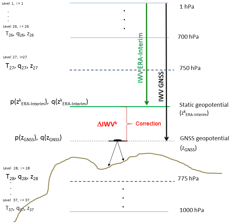
Figure 3 Scheme of the applied correction to the IWV from the ERA-Interim reanalysis for one of the four grid points (k) at a given instant. Both unknowns (z_GNSS, dark gray dashed line, and $z_{\mathrm{NWM}}^k$, thick green line) are located between the pressure levels 27 (750 hPa) and 28 (775 hPa), indicated using thick dashed lines. Atmospheric pressure (p_i), temperature (T_i), specific humidity (q_i) and geopotential (z_i) are known at the 37 levels from 1 to 1000 hPa. Values of $p\left(z_{\text{ERA-Interim}}^k\right)$ and p(z_GNSS) are calculated from Eq. (5), whereas the values of $q\left(z_{\text{ERA-Interim}}^k\right)$ and q(z_GNSS) resulted from a linear interpolation. The computation of ΔIWV^k must be carried out four times ($k=\mathrm{1},\mathrm{\dots },\mathrm{4}$) prior to the bilinear interpolation that produces ΔIWV_ERA-Interim for the given instant.

4 Results

Before analyzing the results of the correction process explained in the previous section, we present a validation of the numerical integration method used. To this end, we calculate the values of IWV_ERA-Interim at each grid point using the numerical integral of Eq. (6). The integration limits range from 1 hPa to the static geopotential value assigned by the model to the point ($z_{\text{ERA-Interim}}^i$). Table 3 shows the results obtained using this procedure. In each grid point the mean value of the differences (IWV_ERA-Interim data – IWV_ERA-Interim calculated) is presented. Standard deviations are also shown. It can be seen that the resulting values are generally very close to zero.

Table 3 Mean values of the difference between IWV_ERA-Interim data and IWV computed from the numerical integral of Eq. (7) at each grid point surrounding the GNSS site. The integration limits range from 1 hPa to the static geopotential value assigned by ERA-Interim to the point ($z_{\text{ERA-Interim}}^k$).

In order to evaluate the improvements introduced by the correction, Fig. 4 shows the $\mathrm{\Delta }\stackrel{\mathrm{‾}}{\mathrm{IWV}}$ as a function of Δz after applying the proposed integral correction to ERA-Interim data. At first glance we can see that, regardless of whether Δz is positive or negative, the differences ($\left|\mathrm{\Delta }\stackrel{\mathrm{‾}}{\mathrm{IWV}}\right|$) decrease to 2 kg m⁻² for all of the stations except in three cases where they barely exceed the abovementioned value. Moreover, the correlation between $\mathrm{\Delta }\stackrel{\mathrm{‾}}{\mathrm{IWV}}$ and the geopotential difference decreases to 0.13, as expected.

Figure 4 Values of $\mathrm{\Delta }\stackrel{\mathrm{‾}}{\mathrm{IWV}}$ ($\mathrm{\Delta }\stackrel{\mathrm{‾}}{\mathrm{IWV}}={\stackrel{\mathrm{‾}}{\mathrm{IWV}}}_{\mathrm{GNSS}}-{\stackrel{\mathrm{‾}}{\mathrm{IWV}}}_{\text{ERA-Interim}}$) as a function of Δz after applying the proposed correction.

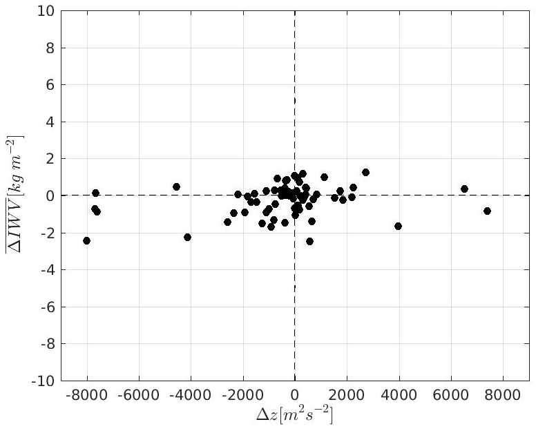
In addition, if we focus on the plot area of Fig. 4 that is limited for a $\mathrm{\Delta }z=\pm \mathrm{1500}$ m² s⁻² and $\mathrm{\Delta }\stackrel{\mathrm{‾}}{\mathrm{IWV}}=\mathrm{1.5}$ kg m⁻² (zoom not shown), we can see that most of the stations (94 %) are included. This shows that the proposed correction decreases $\mathrm{\Delta }\stackrel{\mathrm{‾}}{\mathrm{IWV}}$, even for low stations (small z) that generally have the smallest values of Δz.

The performance of the proposed correction can also be seen in Fig. 5. Where Fig. 5a, c and e show stations with positive Δz, it means that GNSS station is higher than the location assigned by ERA-Interim. Accordingly, the model integrates a thicker layer of atmosphere and, thus, IWV_ERA-Interim values are larger than those from IWV_GNSS. The opposite (Δz is negative) is represented by the sites in Fig. 5b, d and f. Moreover, the differences in Δz are presented increasing from top to bottom in each column in the figure.

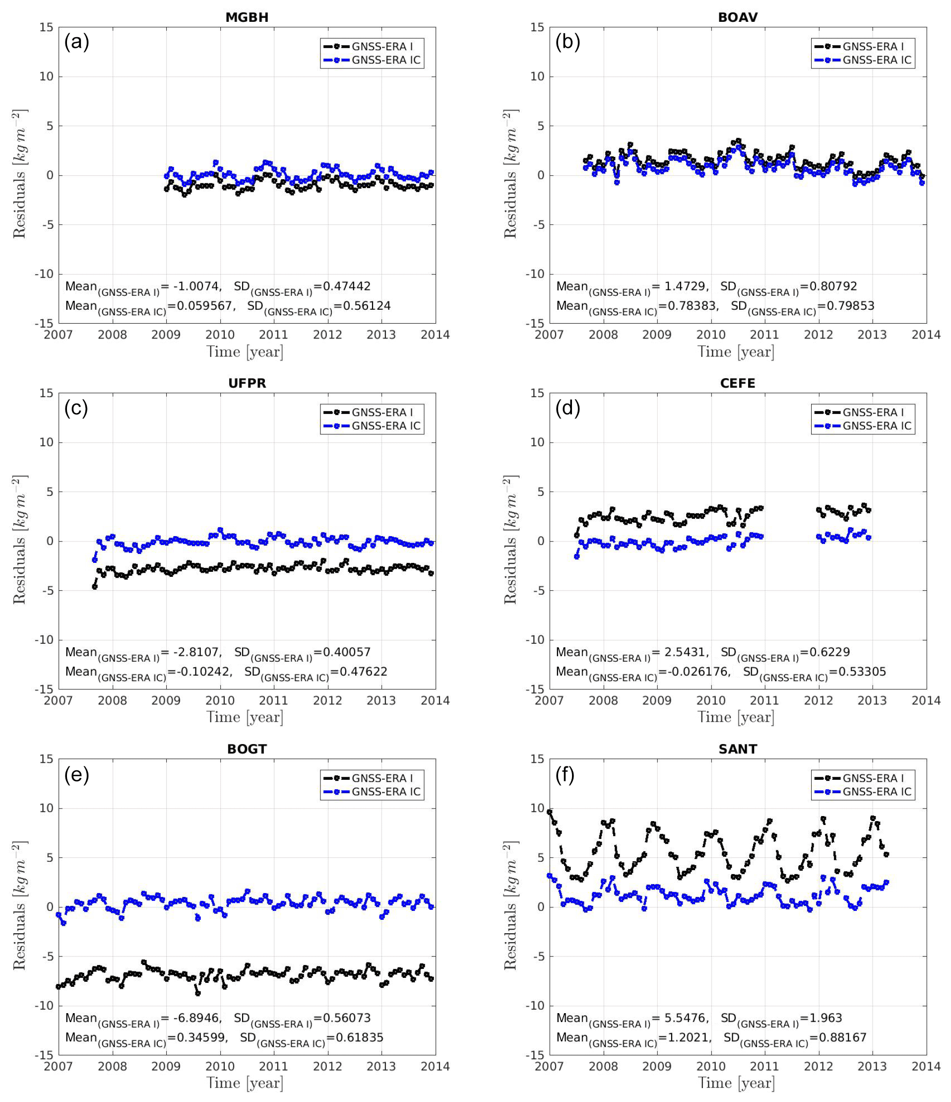
Figure 5 Residuals of the difference between IWV_GNSS and IWV_ERA-Interim (black line) along with residuals of the difference between IWV_GNSS and (IWV_ERA-Interim + correction) (blue line). Panels (a), (c) and (e) show stations with positive Δz, which means that the GNSS station is higher than the location assigned by ERA-Interim; the opposite is shown in panels (b), (d) and (f). Mean values of the residuals along with the standard deviations are also provided. The sites are shown according to Δz decreasing from top to bottom in each column.

We can see that the most important corrections are at BOGT in Bogotá, Colombia, and SANT in Santiago de Chile, Chile. In these examples, the differences (IWV_GNSS−IWV_ERA-Interim), which can reach up to 7 kg m⁻², are significantly reduced.

However the application of this correction, in some cases, should be precautionary. Effectively, sometimes different shortcomings of the model overlap with the height problem; therefore, the proposed correction will not work. For example, in the case of coastal and/or insular stations where two or more grid points are in the ocean: in all of these cases the value of IWV calculated from the bilinear interpolation will be overvalued. Looking at stations near the seashore in more detail (e.g., PARC in Punta Arenas, Chile), where two of the four grid points are in the ocean (see Fig. 6), $\mathrm{\Delta }z=-\mathrm{1271.86}$ at PARC indicates that the geopotential from ERA-Interim is larger than the GNSS geopotential; thus, the proposed correction will be additive. In addition to this result, the IWV_ERA-Interim values are overestimated due to the application of a bilinear interpolation that uses data points located in the ocean. In conclusion, the (IWV_ERA-Interim + correction) value overestimates IWV_GNSS. Thus, this is an example where applying the suggested correction may worsen the results. The same situation is noted at RIO2 at the Argentinean Atlantic coast.

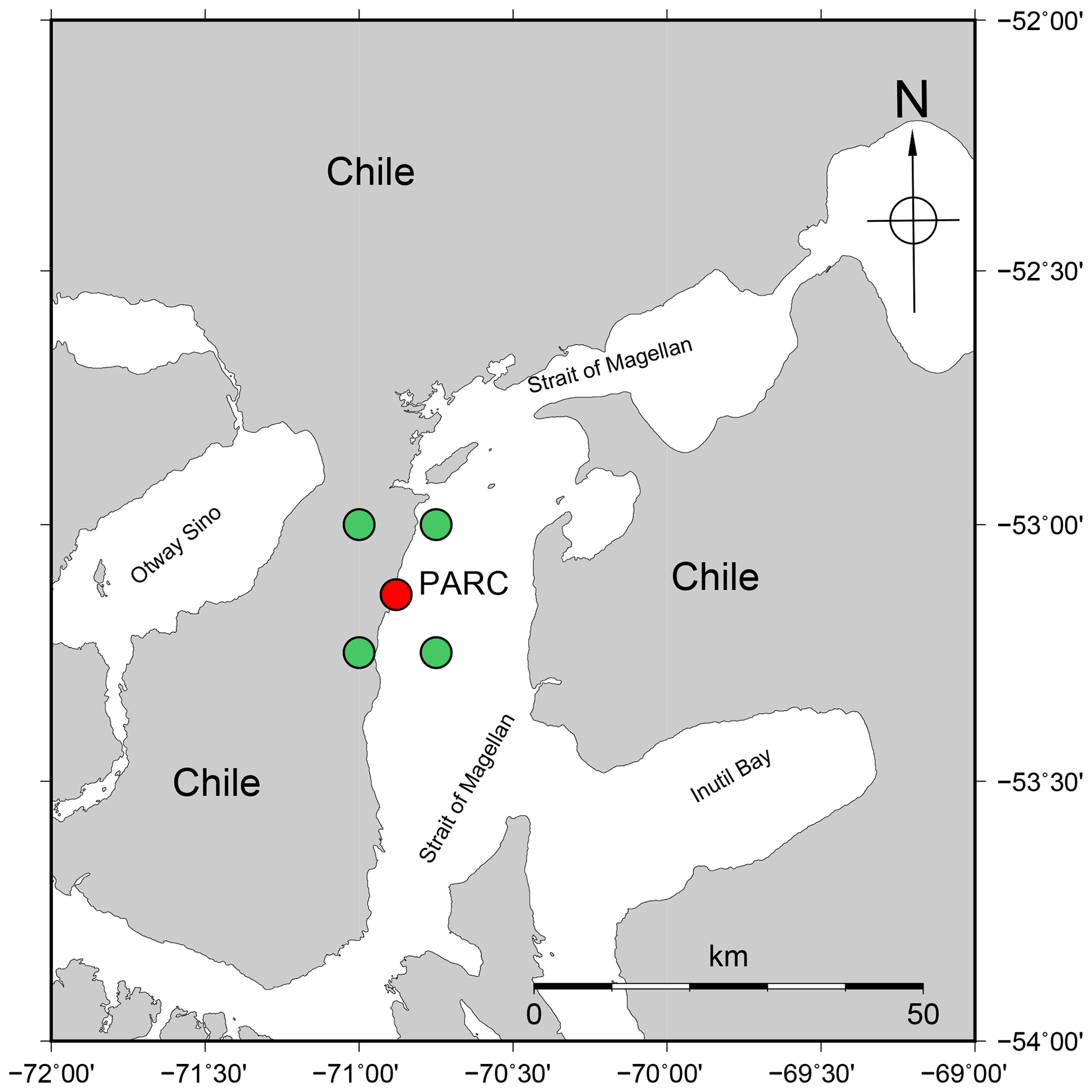
Figure 6 Location of GNSS station PARC along with the four grid points around the station. The grid points correspond to ERA-Interim.

5 Discussion and conclusions

The effect of different heights when comparing results from several data sources not only affects the determination of IWV but also impacts other parameters. For instance, Gao et al. (2012) studied the height corrections for the ERA-Interim 2 m temperature data in the central Alps, and they also found large biases that must be corrected in mountainous areas. Some other authors also studied the tropospheric refraction effects on space geodetic techniques by considering this effect. For example, Teke et al. (2013) performed an inter-technique comparison of ZTD in the framework of four continuous very long baseline interferometry (VLBI) campaigns, including NWM and taking the effect of the height differences into account.

NWM users commonly utilize the IWV values on a grid and use them to calculate the IWV value at a desired location by way of an interpolation method. In this work, taking the values of IWV_GNSS as reference, we show that there are cases where the IWV values obtained from a NWM have differences of several kilograms per square meter and that these discrepancies are mainly due to the difference in geopotentials.

We analyzed the discrepancies between the vertically integrated water vapor values provided by two reanalysis models (ERA-Interim and MERRA-2) with respect to the IWV_GNSS values taken as a reference on the southern and central American continent for the period from 2007 to 2013. The results of this comparison allow us to establish that MERRA-2 results in wetter conditions than GNSS, whereas ERA-Interim is slightly dryer. In addition, when geopotential differences are moderate or large (|Δz|>500 m² s⁻²) and ${\stackrel{\mathrm{‾}}{\mathrm{IWV}}}_{\mathrm{GNSS}}>\mathrm{20}$ kg m⁻², the discrepancies ($\mathrm{\Delta }\stackrel{\mathrm{‾}}{\mathrm{IWV}}$) are greater than 2 kg m⁻² at about 22 % of the stations for both models.

Several authors have reported problems related to the elevation correction for data from the reanalysis models. The artificial bias in the IWV introduced by this altitude difference has previously been reported by Bock et al. (2007), Heise et al. (2009), Van Malderen et al. (2014), Bordi et al. (2014) and Bianchi et al. (2016a).

Heise et al. (2009) derived IWV from global GNSS ZTD at almost 300 sites using ground pressure and temperature values from ECMWF and then compared IWV from GNSS and ECMWF. Similar to our work, they found large discrepancies in mountain regions due to the difference in altitudes that caused errors in the estimations of meteorological values. Moreover, the analysis performed in our work is also in agreement with Bordi et al. (2014), who compared GNSS and ERA-Interim IWV values on a monthly timescale for the period from 2002 to 2012. In this case, the authors found significant biases of 6.4 kg m⁻² in BOGT and 2.5 kg m⁻² in BRAZ, and they related them to the different elevations between the correspondent GNSS site and the grid points of the model. Thus, the values from Bordi et al. (2014) are comparable with the correspondent $\left|\mathrm{\Delta }\stackrel{\mathrm{‾}}{\mathrm{IWV}}\right|$ values estimated in our study (6.87 kg m⁻² in BOGT and 2.03 kg m⁻² in BRAZ, see Table 2).

In this work, we proposed an integral correction that compensates IWV for the effect of the geopotential difference between GNSS and the interpolated grid points in the reanalysis model. The results were tested with the respective values from ERA-Interim. The correction is computed as the numerical integration of the specific humidity where the integral limit is a pressure difference at Δz (see Eq. 7). Considering that 67 % of the stations have $\left|\mathrm{\Delta }\stackrel{\mathrm{‾}}{\mathrm{IWV}}\right|<\mathrm{1.5}$ kg m⁻² for ERA-Interim prior to the correction, the application of the numerical correction improves the results (the percentage of stations below 1.5 kg m⁻² increased to 94 %).

Nevertheless, the application of this correction is not advisable at coastal or insular stations in South and Central America due to the fact that the overvaluation of the model near the coast overlaps with the height problem. These results are in agreement with Ning et al. (2013), who also compared IWV from GNSS with values from two NWMs (ERA-Interim and the Rossby Centre atmospheric climate model – RCA) in Europe for 14 years. The authors also found that models give IWV values larger than GNSS at the seaside or along coasts where the tile of the model includes more than 60 % water.

For this reason, the corrections we propose are always recommended, but they are not advisable at in coastal areas or on islands as at least two grid points of the model are usually in the water.