the Creative Commons Attribution 4.0 License.
the Creative Commons Attribution 4.0 License.
 | 21 Jun 2018
Seasonal characteristics of small- and medium-scale gravity waves in the mesosphere and lower thermosphere over the Brazilian equatorial region
Igo Paulino
Cristiano Max Wrasse
Jose Andre V. Campos
Ana Roberta Paulino
Amauri F. Medeiros
Ricardo Arlen Buriti
Hisao Takahashi
Ebenezer Agyei-Yeboah
Aline N. Lins
The present work reports seasonal characteristics of small- and medium-scale gravity waves in the mesosphere and lower thermosphere (MLT) region. All-sky images of the hydroxyl (NIR-OH) airglow emission layer over São João do Cariri (7.4∘ S, 36.5∘ W; hereafter Cariri) were obtained from September 2000 to December 2010, during a total of 1496 nights. For investigation of the characteristics of small-scale gravity waves (SSGWs) and medium-scale gravity waves (MSGWs), we employed the Fourier two-dimensional (2-D) spectrum and keogram fast Fourier transform (FFT) techniques, respectively. From the 11 years of data, we could observe 2343 SSGW and 537 MSGW events. The horizontal wavelengths of the SSGWs were concentrated between 10 and 35 km, while those of the MSGWs ranged from 50 to 200 km. The observed periods for SSGWs were concentrated around 5 to 20 min, whereas the MSGWs ranged from 20 to 60 min. The observed horizontal phase speeds of SSGWs were distributed around 10 to 60 m s−1, and the corresponding MSGWs were around 20 to 120 m s−1. In summer, autumn, and winter both SSGWs and MSGWs propagated preferentially northeastward and southeastward, while in spring the waves propagated in all directions. The critical level theory of atmospheric gravity waves (AGWs) was applied to study the effects of wind filtering on SSGW and MSGW propagation directions. The SSGWs were more susceptible to wind filtering effects than MSGWs. The average of daily mean outgoing longwave radiation (OLR) was also used to investigate the possible wave source region in the troposphere. The results showed that in summer and autumn, deep convective regions were the possible source mechanism of the AGWs. However, in spring and winter the deep convective regions did not play an important role in the waves observed at Cariri, because they were too far away from the observatory. Therefore, we concluded that the horizontal propagation directions of SSGWs and MSGWs show clear seasonal variations based on the influence of the wind filtering process and wave source location.
Keywords. Atmospheric composition and structure (airglow and aurora) – electromagnetics (wave propagation) – history of geophysics (atmospheric sciences)
Please read the corrigendum first before continuing.
-
Notice on corrigendum
The requested paper has a corresponding corrigendum published. Please read the corrigendum first before downloading the article.
-
Article
(7020 KB)
-
The requested paper has a corresponding corrigendum published. Please read the corrigendum first before downloading the article.
- Article
(7020 KB) - Full-text XML
- Corrigendum
- BibTeX
- EndNote


The study of atmospheric gravity waves (AGWs) is of great importance due to its significant contribution to the dynamics and coupling of the atmospheric layers (Lindzen, 1981; Holton, 1983; Garcia and Solomon, 1985; Alexander and Holton, 1997; Fritts and Alexander, 2003; Yiugit and Medvedev, 2015, 2016). The fundamental understanding of the AGWs has been provided by Hines (1960) who used his theory to interpret the vertical profiles of winds in the mesosphere and lower thermosphere (MLT). AGWs can be categorized as small-scale (SSGWs) and medium-scale (MSGWs). SSGWs are oscillations with horizontal wavelengths less than 100 km and observed period less than 45 min, while MSGWs are oscillations with horizontal wavelengths ranging between several tens and hundreds of kilometers with the observed periods of several tens of minutes to hours (Taylor et al., 2009). These oscillations could be generated by convection, orographic winds, or a wind shear instability process in the atmosphere (Holton, 1992; Alexander and Holton, 1997; Fritts and Alexander, 2003; Tsuda, 2014; Pramitha et al., 2015). Once generated, these oscillations transport energy and momentum in the atmosphere. As the wave propagates upwards, the amplitude of the wave increases due to the exponential decrease in the atmospheric density.
Modeling studies have shown that a significant fraction of the convectively generated MSGWs can propagate above 100 km (Vadas and Fritts, 2004). According to Vadas and Fritts (2004), the AGWs excited by a convective system have a potential to influence the atmosphere at very high altitudes, because they often have relatively long vertical wavelengths and can propagate in all directions from the convective source. They also specified that long vertical wavelengths imply high horizontal phase speeds that escape the critical-level absorption more readily than waves having low phase speeds. Other studies estimated that convective AGWs make a significant contribution to mean forcing in the middle atmosphere (Dunkerton, 1997; Alexander and Holton, 1997; Chun and Baik, 1998; Piani et al., 2000). Further discussion of convection-generated AGWs, and their effects at higher altitudes, can be found in the review by Fritts and Alexander (2003).
Seasonal variations in AGW activities in the MLT region have been studied extensively by all-sky imagers (Wu and Killeen, 1996; Nakamura et al., 1999; Walterscheid et al., 1999; Medeiros et al., 2003; Ejiri et al., 2003; Wrasse et al., 2006a, b; Kim et al., 2010) over the past decades. Wu and Killeen (1996) found that the AGWs activities from OH airglow observations showed a maximum in summer and much weaker activities in winter at the Peach Mountain Observatory, Michigan (42.3∘ N, 83.7∘ W) during 1993 to 1994. Nakamura et al. (1999) observed OH images for 18 months at Shigaraki, Japan (34.9∘ N, 136.1∘ E) from November 1996 to May 1998, and reported that AGWs propagated eastward in summer and westward in winter. Ejiri et al. (2003) used 1-year OH Meinel and OI 557.7 nm band image data at Rikubetsu (43.5∘ N, 143.8∘ E) and Shigaraki from October 1998 to October 1999 and reported that AGWs propagated either northward or northeastward in summer at both sites. However, these waves propagated westward at Rikubetsu and dominantly southwestward at Shigaraki in winter. Kim et al. (2010) used long-term OH Meinel, O2, and OI 557.7 nm band image data at Mt. Bohyun, Korea (36.2∘ N, 128.9∘ E) from July 2001 to September 2005, and found that AGWs showed a preferred propagation direction to the west during autumn and winter and to the east direction during spring and summer. Taylor et al. (1993) also used an all-sky imager to observe wave structure in the NIR-OH nightglow emission at the Mountain Research Station (40.0∘ N, 105.6∘ W; 3050 m) in Colorado. They observed it during the 3-month period (May, June, and July 1988) and found that the wave motions exhibited similar spatial and temporal properties during each month but a distinct tendency for northward propagation with some eastward motion in May and June throughout the campaign. In the Southern Hemisphere, Walterscheid et al. (1999) used the NIR-OH and O2 band image data in Adelaide (35∘ S, 138∘ E), Australia, from April 1995 to January 1996, and presented that most AGWs were possibly thermally ducted, mainly propagating poleward in summer and equatorward in winter.
In the Brazilian low-latitude region, Medeiros et al. (2003) studied the SSGWs patterns seen in the NIR-OH airglow emission using an imaging system operated at Cachoeira Paulista (23∘ S, 45∘ W) from October 1998 to September 1999. According to them, the large-scale waves with horizontal wavelength between 10 and 60 km exhibited a clear seasonal dependence on the horizontal propagation direction, toward southeast in the summer and northwest during the winter. The anisotropy of the propagation direction of the waves were attributed to the effect of wind filtering in the middle atmosphere and the wave source region for the observer. Also in the Brazilian equatorial region, Medeiros et al. (2007) used an all-sky imager for OH, O2, and OI 557.7 nm airglow emission measurements operated at Cariri (7∘ S, 36∘ W) for the observation of SSGWs. The band-type waves showed a clear preference for the horizontal propagation direction from the South American continent to the Atlantic Ocean. Taylor et al. (2009) investigated the general characteristics of both the MSGWs and SSGWs using all-sky imaging measurements of the mesospheric OH emission and the thermospheric OI (630.0 nm) emission at Cariri and Brasilia (14.8∘ S, 47.6∘ W) from 22 September to 9 November 2005.
Although the variety of AGW measurements by optical imagers has been carried out in the last two decades, no systematic study on the characteristics of MSGWs has been performed over the Brazilian equatorial region. For this reason, the present work reports the seasonal characteristics of MSGWs in the MLT region over the Brazilian equatorial sector. MSGWs were determined using NIR-OH airglow images obtained at Cariri and were also compared with the characteristics of SSGWs observed at the same site. The critical level theory of AGWs was applied to study the effects of wind filtering on SSGW and MSGW propagation directions in the middle atmosphere. We also discuss the possible wave source region in the troposphere.
AGWs have been observed using an all-sky image, which is basically composed of a fisheye lens with 180∘ field of view, a telecentric lens system, a filter wheel, and a CCD (charged coupled device) camera. The filter wheel has six slots with 3-inch diameter filters. The integration time to get good airglow images are typically 15 s for the NIR-OH emission (715–930 nm pass band) and 90 s for the OI 577.7 nm, O2, and OI 630.0 nm emissions. The CCD is back illuminated with a resolution of 1024 × 1024 pixels. Each pixel has 24 µm resulting in a total CCD area of 6.03 cm2. The high quantum efficiency (∼ 80 % at visible wavelengths), low dark current (0.5 ), low readout noise (15 electrons rms), and linearity (0.05 %) of the CCD made it possible to achieve quantitative measurements of the airglow emissions (Medeiros et al., 2003). The images are on-chip binned down to 512 × 512 pixels to enhance the signal-to-noise ratio (Medeiros et al., 2003).
The observations were made at Cariri (7.4∘ S, 36.5∘ W) between September 2000 and December 2010, on a total of 1496 nights. Cariri is considered to be one of the driest places in the Brazilian equatorial region, which is good for airglow observations. Figure 1 shows an unwarped OH image projected onto an area of 768 km × 768 km over a map of Brazil. The dashed circle indicates the nominal field of view of the all-sky imager, while the solid lines indicate the magnetic dip latitudes based on the International Geomagnetic Reference Field (IGRF).

Figure 1Map showing the location of Cariri (7.4∘ S, 36.5∘ W) with a NIR-OH unwarped image for a projected area of 768 km × 768 km. The dotted circle indicates the field of view of the imager and the solid lines indicate the magnetic dip latitudes based on the IGRF (International Geomagnetic Reference Field).
Prior to the data analysis, calibration was performed to obtain the lens function of the all-sky imager, which follows the method described by Garcia et al. (1997). The calibrating process can be described as a correction of the spatial coordinates of the images, i.e., the deformation caused by the fisheye lens were minimized and the images were rotated to coincide with the geographical cardinal points. The OH images were first calibrated using the known star background and then projected onto a regular 512 × 512 spatial grid with an assumed peak altitude of 87 km. The lens function was determined by performing a least-square fit using the positions of the stars in the image and the true values of the stars positions obtained from a “star catalog”, for the same location and time of the airglow image. Figure 2 shows an example of the pre-processing technique applied in the present study.
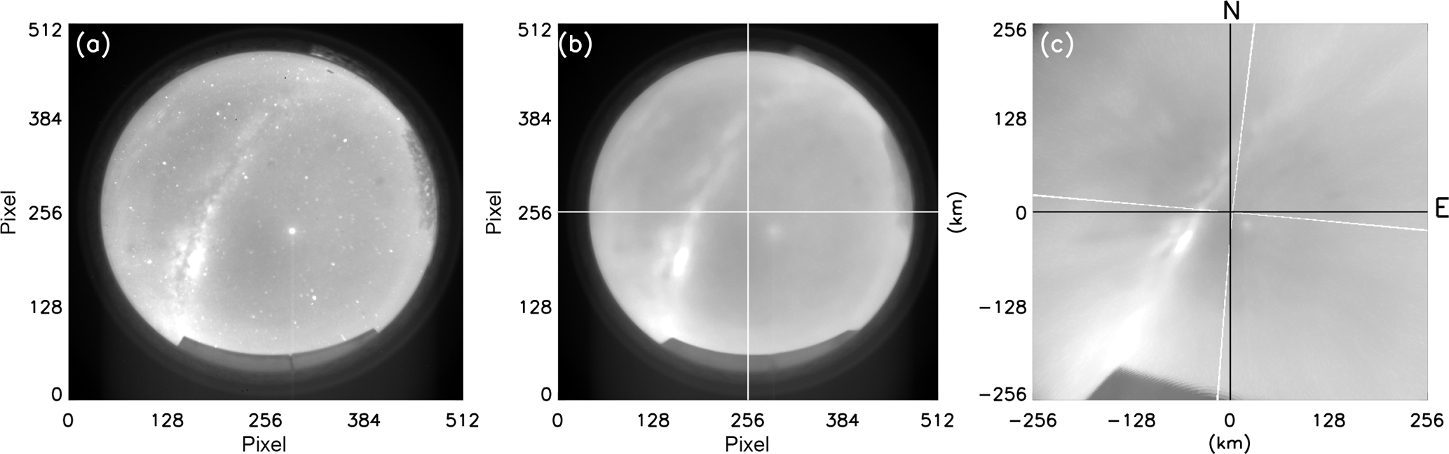
Figure 2Sequence of images showing the pre-processing method used in the AGWs analysis. (a) Raw image of NIR-OH observed on the night of 29 October 2005 over Cariri. (b) The image after the stars have been removed. (c) The linearized and rotated image ready for the FFT analysis.
Figure 2a shows the raw image of NIR-OH observed over Cariri on the night of 29 October 2005. The stars and the tracks of the Milky Way can be noted in the image. Figure 2b shows the image after the stars were removed. Figure 2c presents the linearized rotated image which matches with the geographical coordinates. The black lines illustrate the true north–south and east–west directions, while the white lines are the same as those shown in panel (b). The pre-processing of the images was the same for both SSGWs and MSGWs.
After pre-processing of the all-sky images, it was possible to determine the horizontal wave parameters directly using two techniques to characterize the quasi-monochromatic gravity waves imaged from the NIR-OH airglow emission. The first technique utilized the 2-D spectrum, (Cho, 1995; Medeiros et al., 2003, 2007; Suzuki et al., 2009; Taylor et al., 2009), which focused on quantifying the wave parameters of the small-scale waves (λh≤50 km) that were evident within the images as coherent wave patterns. The horizontal wave parameters were determined directly by investigating AGW content in any part of the image by isolating the region of interest and taking the 2-D fast Fourier transform (FFT) (Medeiros et al., 2007). The determination of the periods (and hence phase speed) of the waves involve taking the one-dimensional (1-D) temporal FFT of the complex 2-D spatial FFT. The peaks in the 1-D FFT correspond to the wave numbers present in the data. Upon this, all the horizontal parameters of the SSGWs (λh, vh, τh) and azimuthal angle (θ), measured from geographic north, were determined.
To investigate the large-scale perturbations in the NIR-OH data, a sequence of images observed in each night were used to create keograms. This was done by extracting a vertical and horizontal slice from the center of individual images, and then spliced them together to create two time series of keograms, showing the zonal and meridional image components. Figure 3 shows the keograms that were created from the set of OH-NIR airglow data observed on the night of 29 October 2005. The panels (a) and (c) show the meridional and zonal components of the keogram, while panels (b) and (d) presented the regions of interest, respectively. There are several coherent linear structures with a clear forward tilt which are the signatures of MSGWs that can be observed between ∼ 19:30 and 23:15 UT (Universal Time). The forward tilt indicates the direction of propagation of the zonal wave component, while the angle of tilt yields its zonal speed. This technique was first employed to study the development and motion of large-scale auroral structures (Eather, 1982), but has been also used to study the wave activity in airglow images on a number of occasions (Swenson et al., 2003; Taylor et al., 2009; Paulino et al., 2011; Suzuki et al., 2013).
The keogram FFT analysis was employed to identify the parameters of MSGWs with λh≥50 km, that were detectable over an extended period of time. A region containing the oscillations was selected in the meridional and zonal keogram components as shown in Fig. 3a and c, respectively. It was ensured that the area of the region to be analyzed was equal in “space-time” in both keogram components. Then, a Fourier transform was applied to get all oscillations with the same period in both time series. Following the methodology of Figueiredo et al. (2018), the wavelength of each meridional and zonal components were determined. Based on the above information, the horizontal wavelength of the wave was estimated. Finally, the phase speed and propagation direction were determined. More details of keogram FFT analysis and the equations involved in the methodology can be found in the appendix of Figueiredo et al. (2018). Applying the keogram FFT analysis on the keogram shown in Fig. 3, it was possible to determine the main characteristics of MSGW, such as λh of 224.8 km, vh of 81.6 m s−1, τh of 45.9 min, and propagated to the northeast direction.

Figure 3Keograms created from a sequence of images observed on the night of 29 October 2005 (MSGWs appear as a coherent, tilted band). The panels (a) and (c) are the meridional and zonal components of the keogram, respectively, while panels (b) and (d) present the regions of interest.
The characteristics of the AGWs present in this section were obtained over a total of 1252 nights with clear skies of airglow observations. The results showed that 2343 SSGW and 537 MSGW events were found in the 11 years of observation. Table 1 presents the yearly distribution of SSGW and MSGW events, clear-sky, cloudy, and observed nights. The highest number of observations with clear-sky nights as well as the SSGW and MSGW events occurred in the year 2009. The details of the statistical distribution can be found in Table 1.
Table 1The yearly distribution of the SSGW and MSGW events, clear-sky, cloudy, and observed nights.
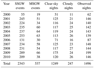
Table 2 shows the monthly distribution of SSGWs and MSGWs in the same way as presented in Table 1. The observations were divided into four periods, November–February, March–April, May–August, and September–October, which corresponds to the Southern Hemisphere summer, autumn, winter, and spring seasons, respectively. The occurrence of SSGWs and MSGWs during the vernal equinox and summer solstice months was higher compared to the autumnal months, while in the winter solstice months the wave activity was lower. This is because the number of nights with clear skies at Cariri was larger in vernal equinoctial months and summer solstice than autumnal equinox and winter solstice. A relatively small number of observations of AGWs in January and February of 2000 and 2006 were due to maintenance of the all-sky imager. It can be noted from Table 2 that spring equinox and summer solstice months presented the largest number of AGW observations. On the other hand, during winter solstice a few AGWs observations were made, due to the rainy season.
Table 2The monthly distribution of the SSGW and MSGW events, clear-sky nights, cloudy nights, and observed nights during the period of 2000 to 2010.
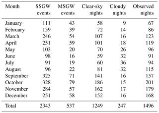
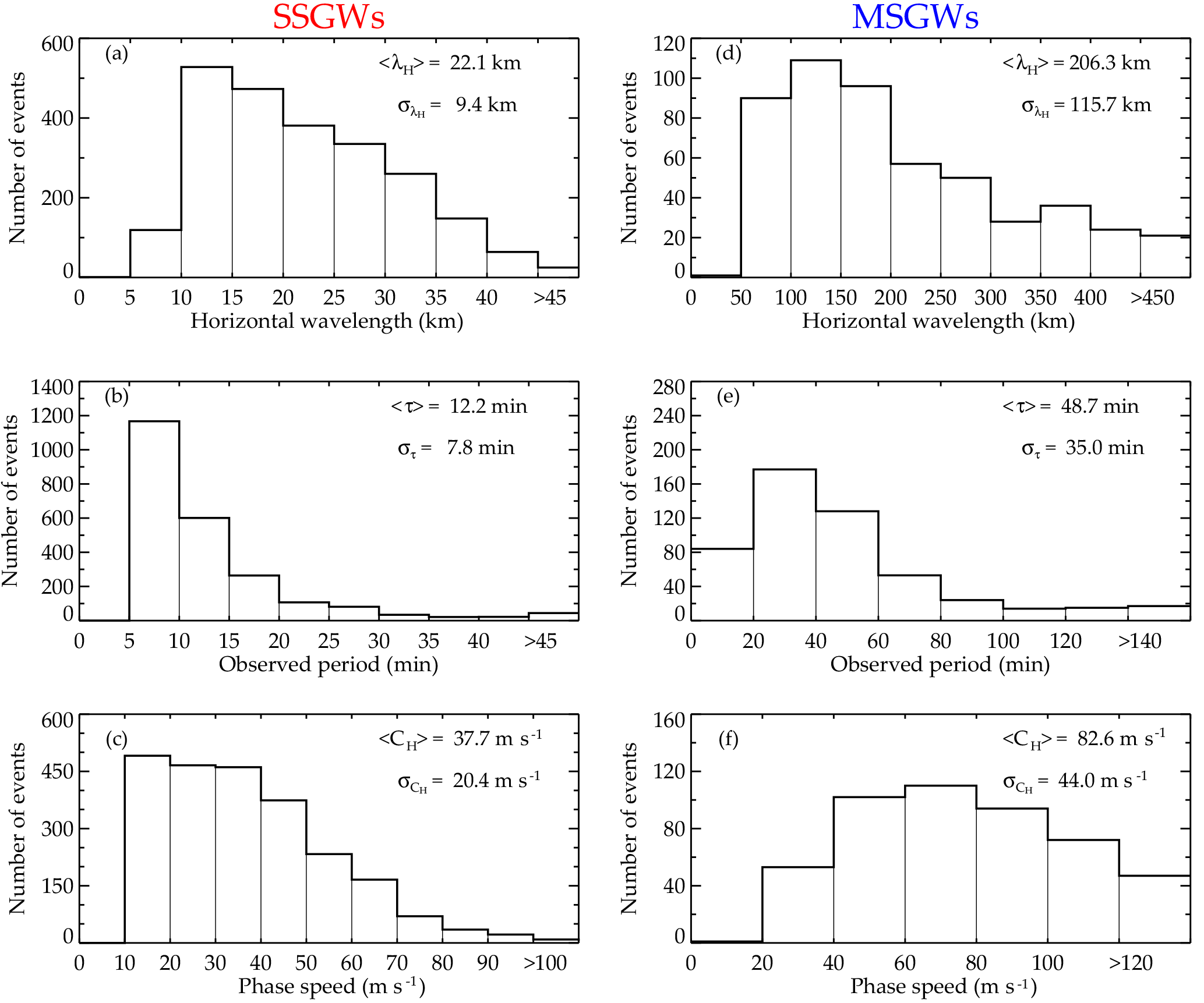
Figure 4 summarizes the following small- and medium-scale gravity wave parameters: horizontal wavelength (λh), period (τh), and the phase speed (vh). The phase speed and period presented in Fig. 4 for both SSGWs and MSGWs are observed parameters, not intrinsic.
4.1 Small-scale AGWs
The histogram in Fig. 4a exhibits the range of horizontal wavelength of SSGWs from 5 to 50 km, with most events distributed from 10 to 35 km and a mean of 22.1 ± 9.4 km. The observed period distribution extended from 5 to 50 min with a maximum peak around 5 to 10 min and a mean of 12.1 ± 7.4 min. The observed phase speed data show a peak around 10 to 70 m s−1 with 20 to 40 m s−1 being the most concentrated range with a mean of 37.6 ± 20.6 m s−1.
In order to study the seasonal variations in the SSGWs over the Brazilian equatorial sector, the occurrences of the wave events have been plotted as a function of propagation direction distribution, as shown in Fig. 5. The overall (total) azimuthal angle shows a strong preference for northeast followed by the southwest and north directions. In summer and autumn most of the wave events propagated in the northeast and southeast directions. However, the results for spring shows that the waves propagate preferentially to the northwest and southeast directions.
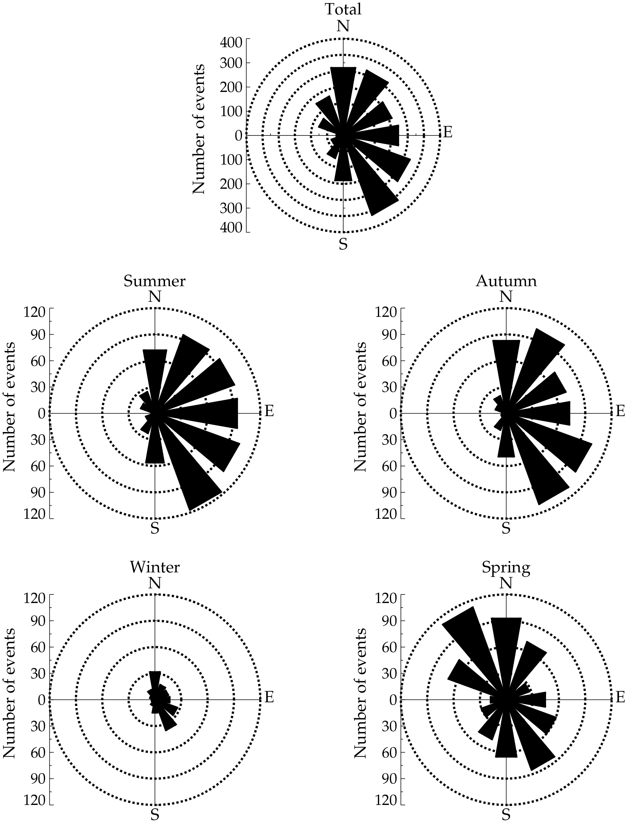
Figure 5The number of SSGW events versus the propagation direction for all 11 years of AGW observations (each bin has 30∘).
4.2 Medium-scale AGWs
In the case of MSGWs, as shown in Fig. 4d the range of horizontal wavelengths extends from 50 to 450 km, in which about 80 % of all MSGWs are within the range of 50 to 300 km, with maximum occurrence between 100 and 150 km. The mean horizontal wavelength is 206.3 ± 115.7 km. Figure 4e shows a clear tendency toward longer observed periods with more than 80 % (429 MSGW events) exhibiting periods between 10 and 80 min, the maximum being concentrated between 20 and 40 min. A few waves have periods more than 80 min. The mean and the standard deviation of the observed period are 48.6 ± 35.1 min. Finally, Fig. 4f shows the distribution of the phase speeds of MSGWs plotted at 20 m s−1 intervals. The measurements range from 20 to 130 m s−1 with the maximum distribution being concentrated between 60 and 80 m s−1. The mean and the standard deviation of the phase speed are 82.6 ± 44.0 m s−1.
The propagation direction of the MSGW events, binned in 30∘ intervals, are plotted in Fig. 6. The total distribution, which is the sum of all MSGW events, shows a clear seasonal variation for the phase propagation direction preferentially to northeast. In summer, autumn, and winter, the MSGWs preferentially propagated northeastward and southeastward, while during spring the waves propagated manly to the northeast and northwest directions.
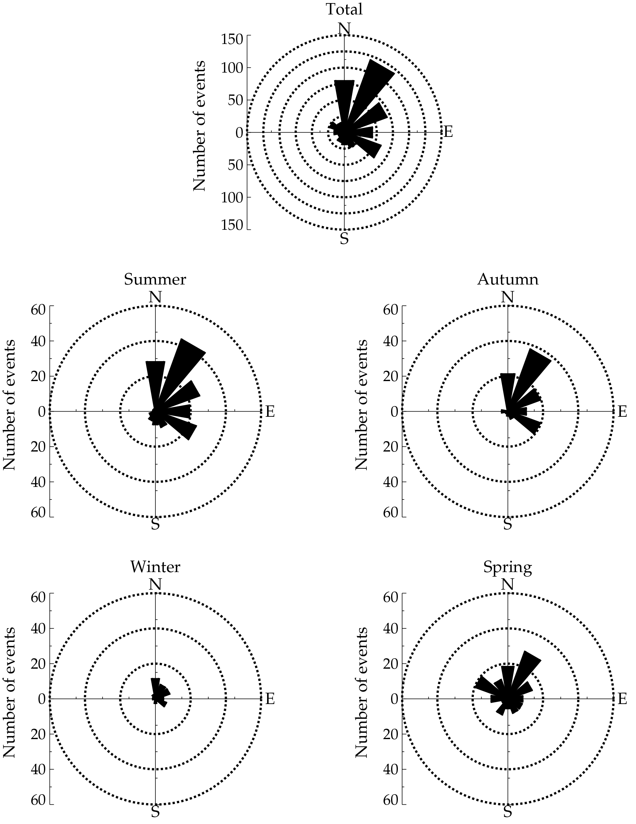
Figure 6The number of MSGW events versus the direction of propagation for all 11 years of AGW observations (each bin has 30∘).
Long-term observation of SSGWs and MSGWs, found in the present work, provides essential information on the characteristics of AGWs, such as scale sizes, occurrences, directionality, and the seasonal variability over the Brazilian equatorial region. Theses gravity wave characteristics will be discussed in more detail in the following sections.
Medeiros et al. (2007)Taylor et al. (2009)Taylor et al. (2009)Medeiros et al. (2003)Bageston et al. (2009)Suzuki et al. (2009)Table 3Summary of the main distribution of SSGW characteristics at different observation sites.
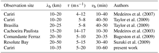
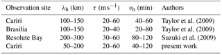
Table 4Summary of the main distribution of MSGW characteristics at different observation sites.
5.1 The horizontal parameters of SSGWs and MSGWs
It was observed that ∼ 200 SSGWs have periods between 5.0 and 8.0 min and they were considered as AGW events. Although the observed periods are shorter than the Brünt–Väissälä (buoyancy) period, which is ∼ 8 to 9 min at ∼ 87 km of altitude (Vadas, 2007), they are considered as AGWs since the criterion of larger than buoyancy period is only applicable to gravity wave intrinsic periods.
Nearly ∼ 475 SSGWs have the observed phase speed below 20 m s−1, which are more susceptible to background wind filtering in the stratosphere and lower mesosphere if we consider that the source mechanism of the waves operated in the troposphere. On the order hand, these events might not be primary propagating AGWs from the lower atmosphere, but could be instability features generated in situ (Taylor et al., 1997; Nakamura et al., 1999).
Table 3 summarizes the average distributions of the characteristics of all the SSGWs observed at Cariri, Cachoeira Paulista (23∘ S, 45∘ W), Brasilia (14.8∘ S, 47.6∘ W), Comandante Ferraz Antarctic Station (62.1∘ S, 58.4∘ W), and Resolute Bay (74.7∘ N, 265.1∘ E) in Canada. At Cariri, Taylor et al. (2009) observed the maximum occurrence of horizontal wavelength around 10 to 20 km, observed period of 5 to 8 min, and the phase speed between 40 and 50 m s−1. Again at Cariri, Medeiros et al. (2007) identified the horizontal wavelengths, observed period, and phase speed around 10 to 20 km, 4 to 12 min, and 10 to 40 m s−1, respectively. In Brasilia, they identified the distribution of horizontal wavelengths around 20 to 25 km, observed period between 5 and 8 min, and phase speed of 40 to 50 m s−1. At Cachoeira Paulista, Medeiros et al. (2003) identified that the main distribution of the horizontal wavelengths, observed period, and phase speed of SSGWs were around 15 to 20 km, 14 to 17 min, and 10 to 30 m s−1, respectively. At Comandante Ferraz Antarctic Station, Bageston et al. (2009) reported that the horizontal wavelengths, observed period, and phase speed were around 20 to 30 km, 5 to 10 min, and 20 to 35 m s−1, respectively. At Resolute Bay in Canada, Suzuki et al. (2009) observed that the occurrence of the horizontal wavelengths, observed period, and phase speed of SSGWs were around 10 to 50 km, 5 to 15 min, and 10 to 50 m s−1, respectively.
In the case of MSGWs, almost 81 events have observed periods below 20 min, that according to Taylor et al. (2009) should be classified as SSGWs. However, in the present work we classified them as MSGWs since their horizontal wavelengths match the criteria of MSGWs (which is λh>100 km).
Table 4 shows a summary of MSGWs average, horizontal wavelengths, observed period, and speed at Cariri, Brasilia, and Resolute Bay. At Cariri, Taylor et al. (2009) identified MSGWs with the maximum distribution of horizontal wavelengths, observed period, and phase speed around 100 to 150 km, 20 to 60 min, and 40 to 60 m s−1, respectively. At Brasilia, Taylor et al. (2009) also reported MSGWs with the main occurrences of horizontal wavelengths, observed period, and phase speed around 100 to 150 km, 20 to 40 min, and 20 to 80 m s−1, respectively. Suzuki et al. (2009) identified the maximum peak of large-scale waves at Resolute Bay with horizontal wavelengths, period, and phase speed of 100 to 400 km, 20 to 60 min, and 40 to 120 m s−1, respectively.
In a general view, most of the SSGWs and MSGWs characteristics reported by the present work, have a wider range of values than those published in previous works (e.g., Medeiros et al., 2007; Taylor et al., 2009, and higher latitudes by Suzuki et al., 2009, and Bageston et al., 2009). The variations in the horizontal parameters of both SSGWs and MSGWs at Cariri might be as a result of the large size of the data set in the present paper or insufficient data of the previous studies. However, the variations in the present results and those from other observation sites could be due to, among others, the differences in the geographical patterns and weak or different local sources (Sato and Yoshiki, 2008; Taylor et al., 2009) of the waves. Moreover, both SSGWs and MSGWs presented in this work are consistent with the previous results of gravity waves as shown in Tables 3 and 4.
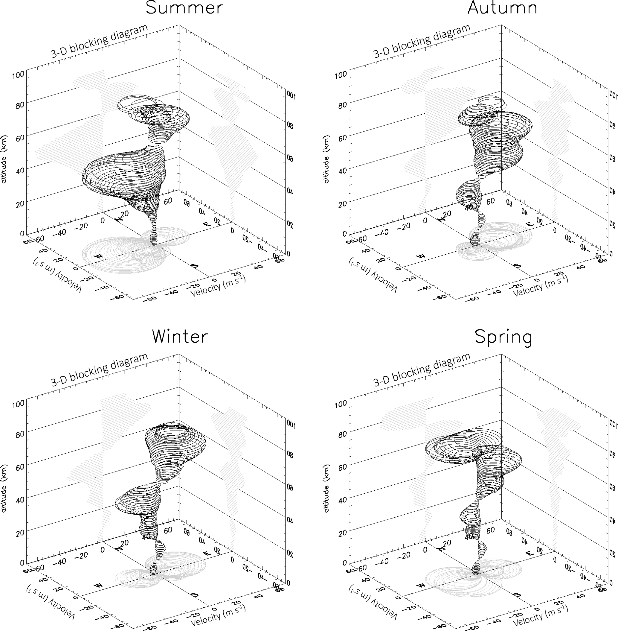
Figure 7Three-dimensional blocking diagrams from 0 to 85 km (critical level projections can be seen at the left and right planes of the 3-D blocking diagram) for summer, autumn, winter, and spring of 2009. The N–S (north–south) axis representing the meridional wind velocity, and E–W (east–west) is the zonal wind velocities derived from the HWM-07 and the vertical axis is the altitude.
5.2 Seasonal variations in SSGW and MSGW propagation directions
AGWs observed at Cariri exhibited almost the same azimuthal distributions within a particular season, irrespective of their horizontal scales. Almost all SSGWs and MSGWs exhibit propagation directions preferentially to the northeast and southeast, as shown in Figs. 5 and 6. However, in spring the SSGWs are propagating in almost all directions, while MSGW seem to propagate to the northeast and northwest directions. These results agree with a previous study done at the same observation site (e.g., Medeiros et al., 2003).
There are two main factors which could create the observed anisotropy of AGW propagation (Fritts et al., 2008). The first one is a AGW filtering process by the background wind, and the second one is the location of the wave source region. AGW propagation direction is a key parameter for understanding the direction and acceleration (or deceleration) of the mean flow (Suzuki et al., 2009).
Winds are an unavoidable feature of a realistic atmosphere. Waves propagating in the direction of the wind flow will be subject to Doppler shifting effects and possible critical level dissipation (Booker and Bretherton, 1967). AGWs propagating upward from the lower atmosphere are liable to be absorbed into the mean flow as they approach a critical level, where the intrinsic frequency of the wave is Doppler shifted to zero. This situation can occur at any height where the wave phase speed is equal to the background wind speed (Medeiros et al., 2003).
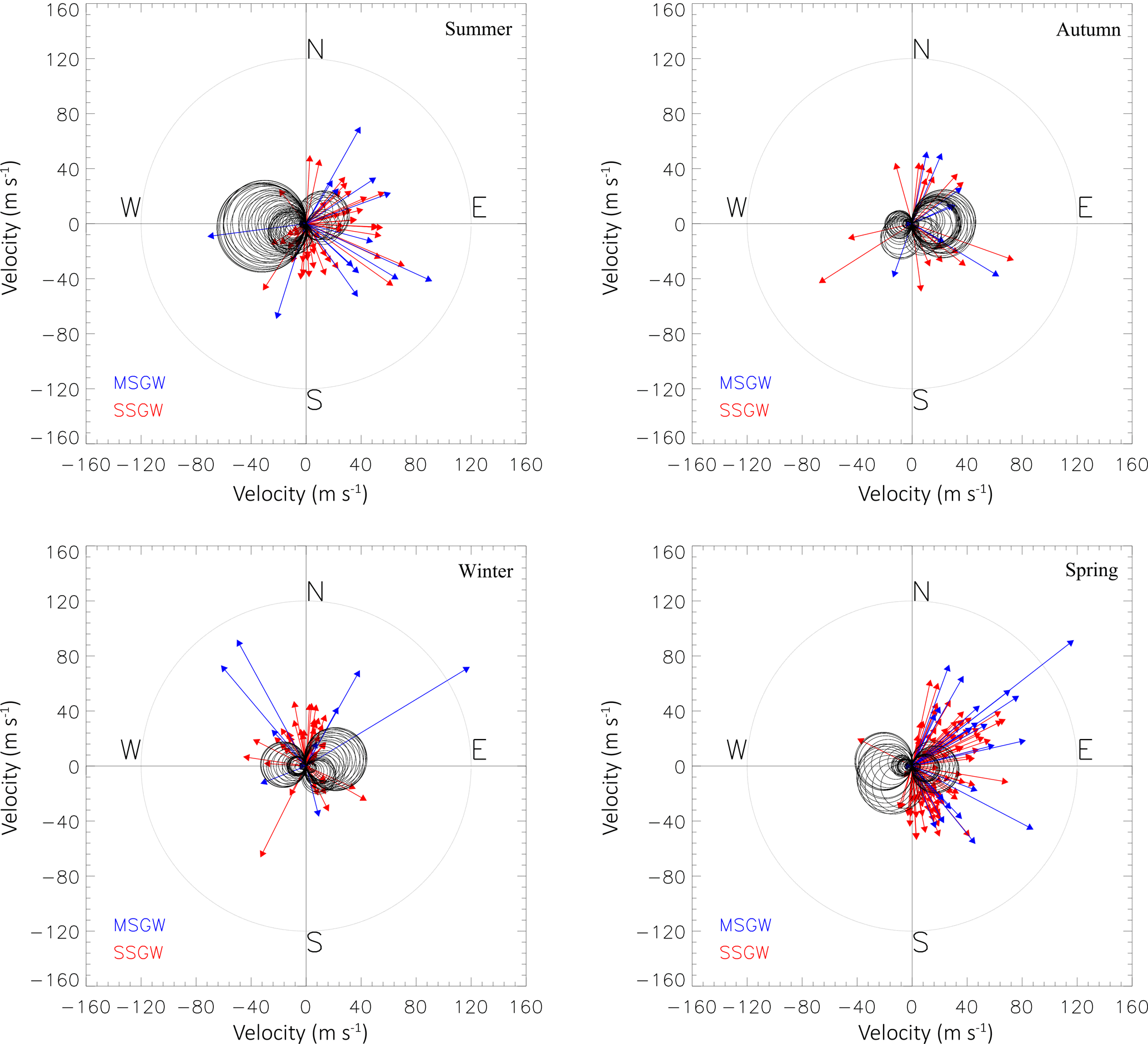
Figure 8Seasonal blocking diagram superimposed with phase speed and the azimuthal angles of SSGWs and MSGWs. The shaded area indicates the magnitude and direction of the restricted region for wave propagation to OH heights. The red and blue arrows show the magnitude and direction of the SSGWs and MSGWs motions, respectively, observed during each season in 2009.
Thus, in order to explain the anisotropy of propagation direction of both SSGWs and MSGWs, we investigate the corresponding wind filtering effects. This can be done by applying the critical level theory of the AGWs filtering (Booker and Bretherton, 1967; Hines and Reddy, 1967; Hazel, 1967; Jones, 1968; Fritts and Geller, 1976; Fritts, 1979). In this way, a horizontal surface can be constructed in a polar plot form, also called blocking diagram, to show the range of azimuthal angles and phase speeds of AGWs that can not propagate upward (Taylor et al., 1993; Zhong et al., 1996; Manson et al., 1999). The Doppler-shifted frequency (Ω) due to the horizontal wind (V0) is given by
where the source frequency is ω, the magnitude of the horizontal wave vector is kx, and V0x is the component of V0 along the wave propagation direction. Equation (1) can be rewritten as
where vx is the observed horizontal phase speed of the AGWs. Equation (2) can be expressed in terms of the zonal (Vz) and meridional wind components (Vm) as the following (Wang and Tuan, 1988; Taylor et al., 1993; Medeiros et al., 2003; Campos et al., 2017):
At the critical level, the gravity wave phase speed equals the background wind speed (V0x=vx and Ω=0); therefore, Eq. (3) can be written as
Equation (4) can be represented in a polar plot of phase speed of the AGWs (vx) for every azimuth when the zonal (Vz) and meridional wind components (Vm) are known. Therefore, in order to analyze the seasonal variation in the critical level effects on the propagation direction of AGWs, the above methodology has been used to plot blocking diagrams for each season using the wind profiles from the Horizontal Wind Model 2007 (HWM-07; Drob et al., 2008).
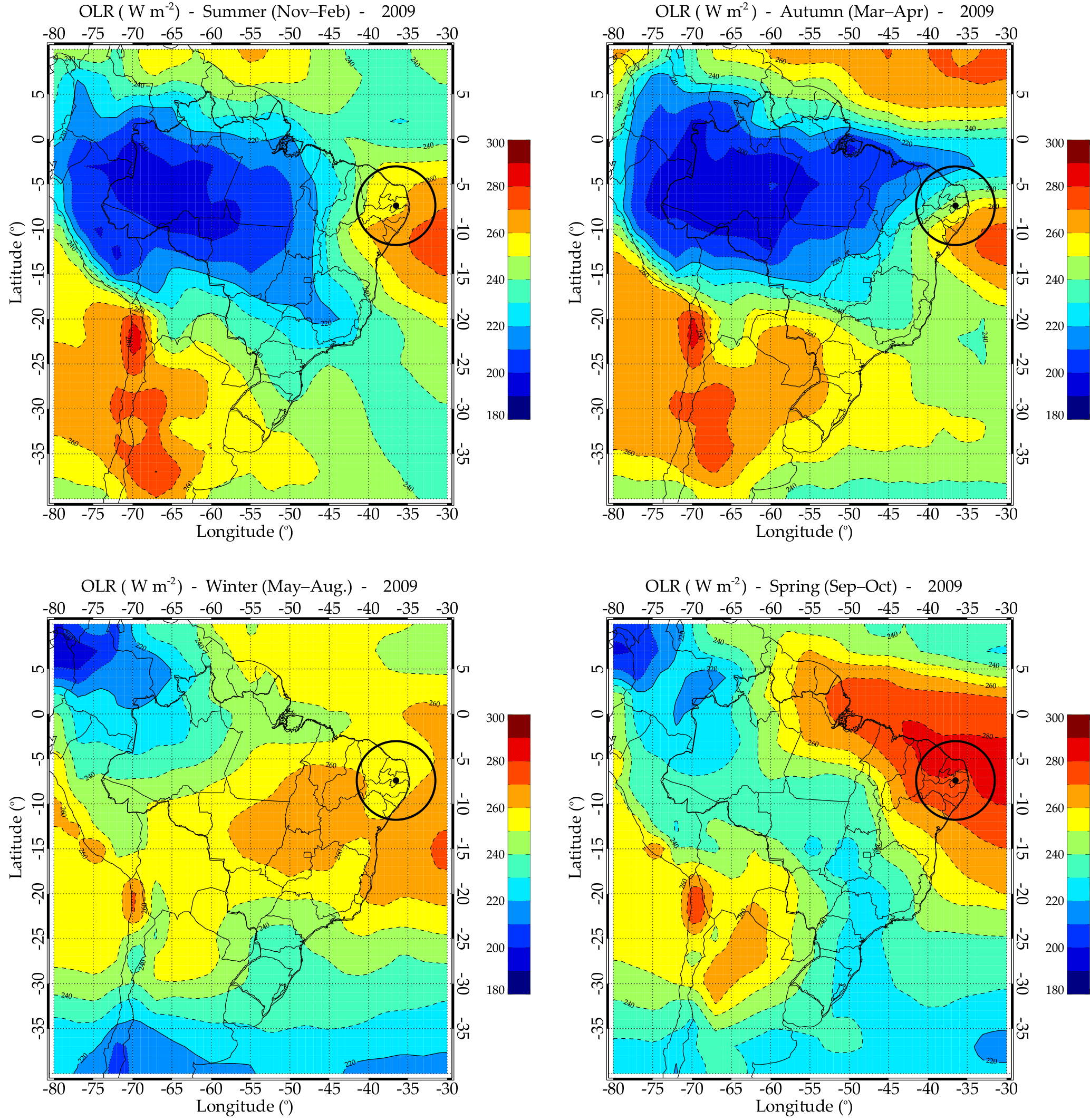
Figure 9The average daily mean of the outgoing longwave radiation (OLR, in W m−2) over South America for each season in 2009 during AGW observations at Cariri.
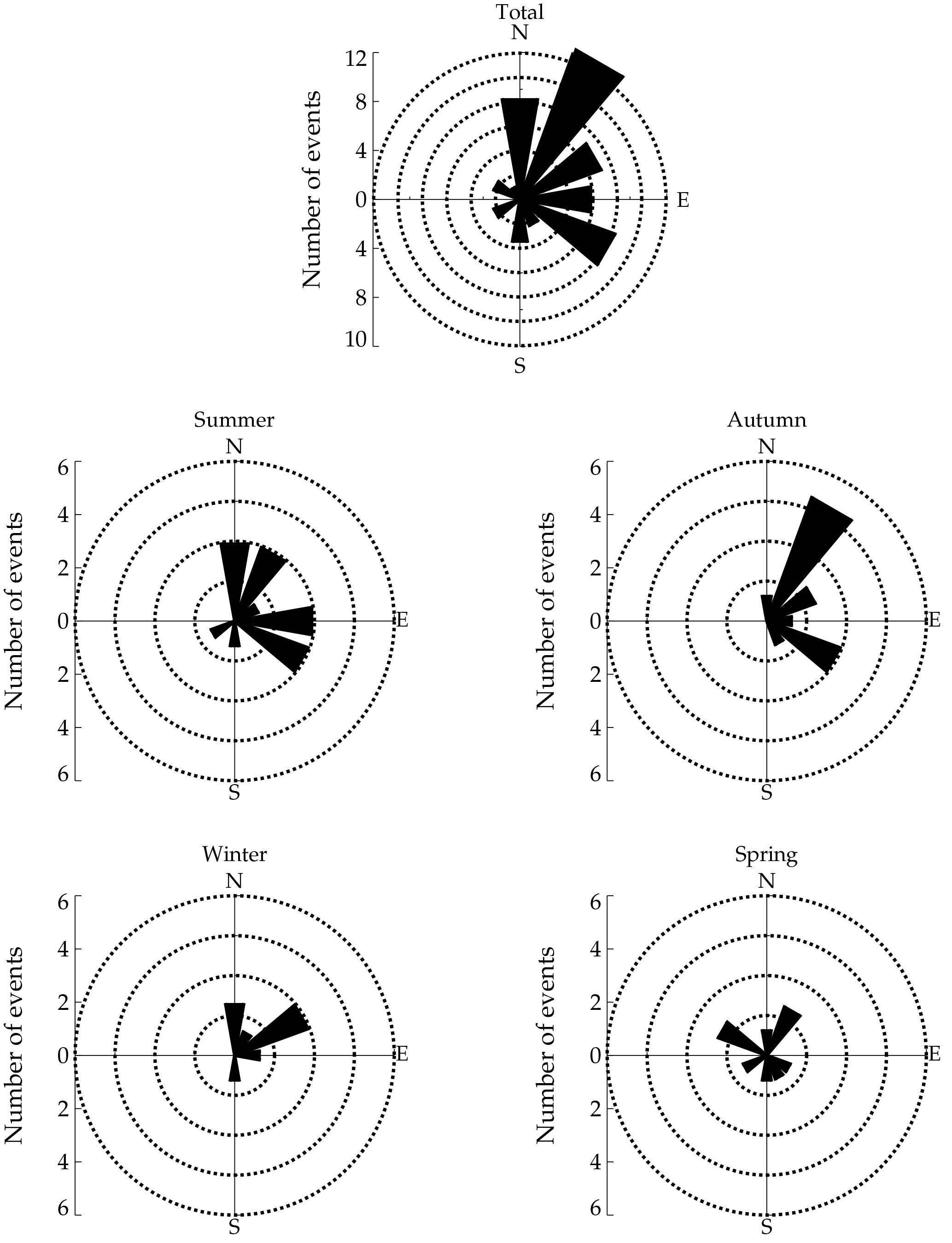
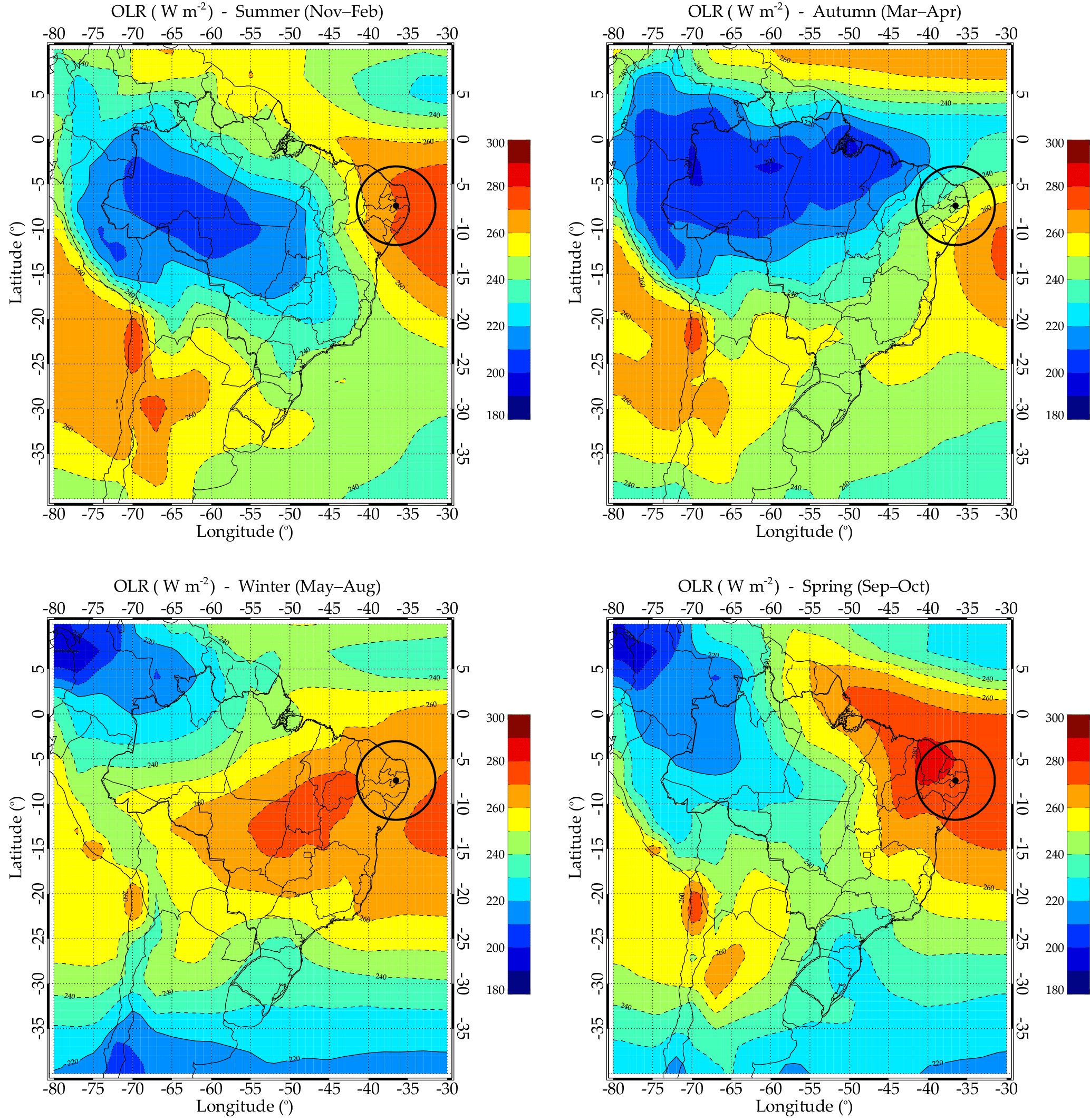
Figure 11Seasonal variation in 11 years of daily mean of outgoing longwave radiation (OLR) over South America.
Figure 7 shows a background wind blocking diagram from 0 to 85 km for different seasons. In this figure each circle represents the critical level of AGW vertical propagation. The projections of the critical level profile can be seen at the left and right planes of the 3-D blocking diagram.
The behavior of the wind profile shows a clear seasonal variation. Each season shows a critical level at east–west directions due to the strong zonal wind in the stratosphere and lower mesosphere. For example, in summer and spring, the wind propagates westward with maximum velocity between 40 and 60 km and between 70 and 85 km of altitude, respectively. However, in autumn and winter, the winds were directed westward and eastward with maximum wind velocity between 50 and 80 km and between 70 to 85 km of altitude, respectively. We chose an example of blocking diagram for the year 2009, due to the larger number of both SSGW and MSGW observations. Similar features of seasonal variation for the blocking diagram were also noticed in the other years.
The seasonal variations in the background wind have been studied concerning SSGW and MSGW events in 2009. In this case, the phase speed and azimuthal angles of the wave were plotted as radial lines versus polar angles to show magnitudes and directions, respectively. Figure 8 shows the blocking diagrams superimposed with phase speed and the azimuthal angles of propagation of the SSGWs and MSGWs observed in NIR-OH airglow emissions for different seasons during 2009. The shaded area indicates the magnitude and direction of the critical level for the upward propagation of the AGWs. The red (SSGWs) and blue (MSGWs) arrows show the magnitude and direction of the SSGWs and MSGWs motions, respectively.
It can be noted in Fig. 8 that the wind effect decreases considerably in an area from summer to spring, eventually restricting all zonal propagating SSGWs and MSGWs with observed phase speed less than or equal to the magnitude of the background wind. For instance, in summer and spring, the background wind directions at the critical level was opposite to the phase propagation direction of the waves. Therefore, eastward waves were not filtered out by the background wind. On the order hand, westward waves with a phase speed lower than ∼ 70 m s−1 in the summer and ∼ 40 m s−1 in the spring were filtered by the mean flow. It can be seen that in winter and autumn, eastward waves with phase speeds lower than ∼ 50 m s−1 were absorbed by the wind. Likewise the westward waves with phase speed lower than ∼ 35 m s−1 in winter and ∼ 25 m s−1 in autumn were also absorbed by the background wind. Meanwhile, waves propagating toward the north and south directions were generally less restricted; therefore, they propagated to the NIR-OH layer to be observed. On the order hand, all the zonal propagated waves trapped in the critical level could not propagate further upward to the OH emission layer to be observed. However, all the waves that were observed in the OH emission layer, with phase speeds lower or equal to that of the speed of the background wind, were generated in situ.
Although the critical level filters the AGWs and entirely prevents them from propagating vertically in the atmosphere, a small Doppler frequency shift may work in the wave's favor, by helping it to propagate to the higher altitudes, or unfavorable to the waves, resulting in premature ducting or reflection. Therefore, it is obvious that winds do not hinder the propagation of AGWs entirely. Hecht et al. (2001) reported that the winds orthogonal to the propagation direction of the AGWs will not entirely result in premature reflection or dissipation. For example, with predominantly northeastward and southeastward directionality of SSGWs and MSGWs in the present paper, most of the waves propagated in directions that were least impeded by the zonal wind. The majority of the MSGWs were less susceptible to wind filtering effects because of their larger scale sizes as indicated by their higher phase speeds. Such waves are better suited for ray tracing studies to identify their potential sources and also irregularities that they can trigger in the ionosphere (Vadas et al., 2009; Barros et al., 2018).
The influence of the background wind filtering alone cannot justify the directionality of the phase propagation of AGWs over Cariri; therefore, the source regions must also be investigated. According to Fritts et al. (2008), the source region of the AGWs can be anisotropic, that is either for each individual source or for the location of the sources relative to the observer. Thus, the SSGWs and MSGWs have been studied in relation to a deep convective process in the troposphere to identify the possible source regions of the waves in each season. The outgoing longwave radiation (OLR) data were obtained from the National Oceanic and Atmospheric Administration (NOAA) to localize the deep convective regions. Figure 9 shows the seasonal average of daily mean OLR over South America for 2009 and the corresponding azimuthal angles of plots of MSGWs are shown in Fig. 10. The site location is represented by a circle on the map. The temperature of less than 200 K corresponds to the deep convection (Sivakandan et al., 2016). Almost the same characteristics of seasonal variation for the deep convection were realized in the other years. Since the deep convective profile for each season does not show significant changes during the years, we chose to represent the plot of 2009 and the corresponding MSGWs propagation directions.
It is noted from Fig. 9 that during the autumn and summer, there were deep convection processes occurring mainly at the northwest and southwest directions of the observation site. These were the possible generation mechanism of the waves that propagated from these source regions to the OH airglow emission layer. Coincidentally, most of the waves observed in that same season were propagating toward northeast and southeast directions, away from the deep convection, as shown in Fig. 10. This shows that tropospheric convection was the possible source for generation of SSGWs and MSGWs observed. Alexander and Vincent (2000) concluded that the seasonal and interannual variability in AGWs observed at Cocos Island was likely due to deep convection. Therefore, the changing AGWs source region for the observer is very important to explain the anisotropy in the Brazilian equatorial region where the zonal winds are weak except in summer (Medeiros et al., 2003, 2007). The source region with respect to Cariri is an important determining factor of the propagation direction which can not be underestimated.
On the order hand, the deep convection process in spring and winter appeared at a distance greater than 3000 km in the Amazon Forest, which is the far northwestern part of Cariri. In the absence of background winds, AGWs of a period of ≤ 1 h would be expected to propagate from the source region to OH heights within a ground range of ∼ 800 km (Freund and Jacka, 1979; Taylor and Hapgood, 1988). However, as the path of the gravity wave through the atmosphere is strongly dependent upon its intrinsic frequency (Hines, 1960), which changes with the prevailing wind conditions, the horizontal range over which the waves may propagate can be significantly larger. Vadas (2007) also used a ray trace model to explore AGW properties that resulted from a wide range of temperatures, calculating the dissipation altitudes, horizontal distances traveled, times taken, and maximum horizontal wavelengths prior to dissipation for a wide range of upward-propagating AGWs that originate in the lower atmosphere and at several altitudes. They reported that, for AGWs to travel horizontally for ∼ 3000 km, it should posses a horizontal wavelength between 600 and 800 km, time taken for horizontal propagation between 4 and 5 h, and the phase speed between 150 and 250 m s−1. Although, it is possible that many of the wave motions imaged by the all-sky camera at Cariri might have originated from sources located several hundred kilometers from the observing site, the horizontal parameters of SSGWs and MSGWs in the present paper are not enough to cover that ground range. Thus, it is impossible for such a distant convective process to be the seeding mechanism for the observed AGWs in spring and winter at Cariri. They might be triggered by other processes that have to be explored. The seasonal variation in 11 years of daily mean of OLR, shown in Fig. 11, proves likewise that during spring and winter AGWs can not be attributed to the deep convection as a possible source mechanism.
Eleven years of AGW observations were made from NIR-OH emissions using an all-sky airglow imager at Cariri (7.4∘ S, 36.5∘ W). The measurements were made from September 2000 to December 2010 with a total of 1252 nights of clear sky. For investigation of the seasonal characteristics of SSGWs and MSGWs, we employed the Fourier 2-D spectrum and keogram FFT techniques on a total of 2343 and 537 events, respectively. The range of the horizontal wavelengths of SSGWs were concentrated between 5 and 50 km with most events distributed from 10 to 35 km, while that of MSGWs ranged from 50 to 450 km with maximum distribution around 50 to 200 km. The corresponding mean of all horizontal wavelengths of SSGWs and MSGWs were 22.1 ± 9.4 and 206.3 ± 115.7 km, respectively. The observed periods of SSGWs extended from 5 to 50 min with a maximum peak around 5 to 10 min, whereas MSGWs ranged from 10 to 150 min with maximum occurrence from 20 to 60 min. The mean of all periods of SSGWs and MSGWs are 12.2 ± 7.8 and 48.7 ± 35.0 min, respectively. Also, the observed phase speeds of SSGWs were distributed around 10 to 70 m s−1 with most frequent waves between 20 and 40 m s−1, while MSGWs ranged from 20 to 130 m s−1 with the maximum occurrence between 60 and 80 m s−1. The mean of all phase speeds were 37.7 ± 20.6 and 82.6 ± 44.0 m s−1 for SSGWs and MSGWs, respectively. In the 11 years of AGW observations, SSGWs show propagation directions preferentially northeast and southeast, whereas the MSGWs propagate preferentially in the northeast direction. In summer, autumn, and winter both SSGWs and MSGWs preferentially propagated northeastward and southeastward, while in spring the waves propagated in all directions. The critical level theory of AGWs was applied to study the effects of wind filtering on SSGW and MSGW propagation directions. We realized that the anisotropy of the propagation direction of both SSGWs and MSGWs was as a result of a wind filtering process acting on AGWs in the middle atmosphere. Moreover, the SSGWs were more susceptible to wind filtering effects than MSGWs. Furthermore, the average of daily mean OLR was used to investigate the possible wave source region in the troposphere. The results showed that in summer and autumn, deep convective regions were the possible source mechanism of the AGWs. However, in spring and winter the deep convective regions did not play an important role in the waves observed at Cariri, because they were too far away from the observation site. Therefore, the horizontal propagation directions of SSGWs and MSGWs show clear seasonal variations based on the influence of the wind filtering process and wave source location.
The data used to produce the results of this manuscript were obtained from the “Observatório de Luminescência Atmosférica da Paraíba” at São João do Cariri, which is supported by the Universidade Federal de Campina Grande and Instituto Nacional de Pesquisas Espaciais. If someone would like to access these data, please contact either Amauri F. Medeiros (afragoso@df.ufcg.edu.br) or Hisao Takahashi (hisao.takahashi@inpe.br).
The authors declare that they have no conflict of interest.
This article is part of the special issue “Space weather connections to near-Earth space and the atmosphere”. It is a result of the 6∘ Simpósio Brasileiro de Geofísica Espacial e Aeronomia (SBGEA), Jataí, Brazil, 26–30 September 2016.
Thanks to the Coordenação de Aperfeiçoamento de Pessoal de Nível Superior (CAPES) and Conselho Nacional de Desenvolvimento Científico e Tecnológico (CNPq) for the scholarship and also the support offered by CNPq under the following contracts; 460624/2014-8, 473473/2013-5, 301078/2013-0, 478117/2013-2, and 310926/2014-9.
We are grateful to Observatório de Luminescência Atmosférica da Paraíba
at São João do Cariri, Universidade Federal de Campina Grande, and the Instituto
Nacional de Pesquisas Espaciais for making the data in this paper available. We are
most grateful to Cosme Alexandre Oliveira Barros Figueiredo and Diego Barros
for helping in responding to reviewers and topical editors reports.
The topical editor, Mangalathayil Abdu, thanks four anonymous referees for help in evaluating this paper.
Alexander, M. J. and Holton, J. R.: A model study of zonal forcing in the equatorial stratosphere by convectively induced gravity waves, J. Atmos. Sci., 54, 408–419, https://doi.org/10.1175/1520-0469(1997)054<0408:AMSOZF>2.0.CO;2, 1997. a, b, c
Alexander, M. J. and Vincent, R. A.: Gravity waves in the tropical lower stratosphere: A model study of seasonal and interannual variability, J. Geophys. Res.-Atmos., 105, 17983–17993, https://doi.org/10.1029/2000JD900197, 2000. a
Bageston, J. V., Wrasse, C. M., Gobbi, D., Takahashi, H., and Souza, P. B.: Observation of mesospheric gravity waves at Comandante Ferraz Antarctica Station (62∘ S), Ann. Geophys., 27, 2593–2598, https://doi.org/10.5194/angeo-27-2593-2009, 2009. a, b, c
Barros, D., Takahashi, H., Wrasse, C. M., and Figueiredo, C. A. O. B.: Characteristics of equatorial plasma bubbles observed by TEC map based on ground-based GNSS receivers over South America, Ann. Geophys., 36, 91–100, https://doi.org/10.5194/angeo-36-91-2018, 2018. a
Booker, J. R. and Bretherton, F. P.: The critical layer for internal gravity waves in a shear flow, J. Fluid Mech., 27, 513–539, https://doi.org/10.1029/2000JD900197, 1967. a, b
Campos, J. A. V., Paulino, I., Wrasse, C., Medeiros, A. F., Paulino, A. R., and Buriti, R.: Observations of small-scale gravity waves in the equatorial upper mesosphere, Brazilian Journal of Geophysics, 34, 472, https://doi.org/10.22564/rbgf.v34i4.876, 2017. a
Cho, J. Y. N.: Inertio-gravity wave parameter estimation from cross-spectral analysis, J. Geogphys. Res., 100, 18727–18737, https://doi.org/10.1029/95JD01752, 1995. a
Chun, H.-Y. and Baik, J.-J.: Momentum flux by thermally induced internal gravity waves and its approximation for large-scale models, J. Atmos. Sci., 55, 3299–3310, https://doi.org/10.1175/1520-0469(1998)055<3299:MFBTII>2.0.CO;2, 1998. a
Drob, D. P., Emmert, J. T., Crowley, G., Picone, J. M., Shepherd, G. G., Skinner, W., Hays, P., Niciejewski, R. J., Larsen, M., She, C. Y., Meriwether, J. W., Hernandez, G., Jarvis, M. J., Sipler, D. P., Tepley, C. A., O'Brien, M. S., Bowman, J. R., Wu, Q., Murayama, Y., Kawamura, S., Reid, I. M., and Vincent, R. A.: An empirical model of the Earth's horizontal wind fields: HWM07, J. Geophys. Res.-Space Phys., 113, 4–13, https://doi.org/10.1029/2008JA013668, 2008. a
Dunkerton, T. J.: The role of gravity waves in the quasi-biennial oscillation, J. Geophys. Res.-Atmos., 102, 26053–26076, https://doi.org/10.1029/96JD02999, 1997. a
Eather, R. H.: Dayside aurora studies with a color keogram camera, Antarct. J. U.S., 17, 218, 1982. a
Ejiri, M. K., Shiokawa, K., Ogawa, T., Igarashi, K., Nakamura, T., and Tsuda, T.: Statistical study of short-period gravity waves in OH and OI nightglow images at two separated sites, J. Geophys. Res.-Atmos., 108, 5–7, https://doi.org/10.1029/2002JD002795, 2003. a, b
Figueiredo, C. A. O. B., Takahashi, H., Wrasse, C. M., Otsuka, Y., Shiokawa, K., and Barros, D.: Medium scale traveling ionospheric disturbances observed by detrended total electron content maps over BrazilMedium scale traveling ionospheric disturbances observed by detrended total electron content maps over Brazil, J. Geophys. Res.-Space Phys., 123, 20–22, https://doi.org/10.1002/2017JA025021, 2018. a, b
Freund, J. T. and Jacka, F.: Structure in the lambda 557.7 nm [OI] airglow, J. Atmos. Terr. Phys., 41, 25–31, https://doi.org/10.1016/0021-9169(79)90043-6, 1979. a
Fritts, D. C.: The excitation of radiating waves and Kelvin-Helmholtz instabilities by the gravity wave-critical level interaction, J. Atmos. Sci., 36, 12–23, https://doi.org/10.1175/1520-0469(1979)036<0012:TEORWA>2.0.CO;2, 1979. a
Fritts, D. C. and Alexander, M. J.: Gravity wave dynamics and effects in the middle atmosphere, Rev. Geophys., 41, 9–10, https://doi.org/10.1029/2012RG000409, 2003. a, b, c
Fritts, D. C. and Geller, M. A.: Viscous stabilization of gravity wave critical level flows, J. Atmos. Sci., 33, 2276–2284, https://doi.org/10.1175/1520-0469(1976)033<2276:VSOGWC>2.0.CO;2, 1976. a
Fritts, D. C., Vadas, S. L., Riggin, D. M., Abdu, M. A., Batista, I. S., Takahashi, H., Medeiros, A., Kamalabadi, F., Liu, H.-L., Fejer, B. G., and Taylor, M. J.: Gravity wave and tidal influences on equatorial spread F based on observations during the Spread F Experiment (SpreadFEx), Ann. Geophys., 26, 3235–3252, https://doi.org/10.5194/angeo-26-3235-2008, 2008. a, b
Garcia, F. J., Taylor, M. J., and Kelley, M. C.: Two-dimensional spectral analysis of mesospheric airglow image data, Appl. Optics, 36, 7374–7385, 1997. a
Garcia, R. R. and Solomon, S.: The effect of breaking gravity waves on the dynamics and chemical composition of the mesosphere and lower thermosphere, J. Geophys. Res.-Atmos., 90, 3850–3868, https://doi.org/10.1029/JD090iD02p03850, 1985. a
Hazel, P.: The effect of viscosity and heat conduction on internal gravity waves at a critical level, J. Fluid Mech., 30, 775–783, https://doi.org/10.1017/S0022112067001752, 1967. a
Hecht, J. H., Walterscheid, R. L., Hickey, M. P., and Franke, S. J.: Climatology and modeling of quasi-monochromatic atmospheric gravity waves observed over Urbana Illinois, J. Geophys. Res.-Atmos., 106, 5181–5195, https://doi.org/10.1029/2000JD900722, 2001. a
Hines, C. and Reddy, C. A.: On the propagation of atmospheric gravity waves through regions of wind shear, J. Geophys. Res., 72, 1015–1034, https://doi.org/10.1029/JZ072i003p01015, 1967. a
Hines, C. O.: Internal atmospheric gravity waves at ionospheric heights, Can. J. Phys., 38, 1441–1481, https://doi.org/10.1139/p60-150, 1960. a, b
Holton, J. R.: The influence of gravity wave breaking on the general circulation of the middle atmosphere, J. Atmos. Sci., 40, 2497–2507, https://doi.org/10.1175/1520-0469(1983)040<2497:TIOGWB>2.0.CO;2, 1983. a
Holton, J. R.: An introduction to dynamic meteorology, International geophysics series, San Diego, New York, 107, 184–206, https://doi.org/10.1002/qj.49710745218, 1992. a
Jones, W. L.: Reflexion and stability of waves in stably stratified fluids with shear flow: A numerical study, J. Fluid Mech., 34, 609–624, https://doi.org/10.1017/S0022112068002119, 1968. a
Kim, Y. H., Lee, C., Chung, J.-K., Kim, J.-H., and Chun, H.-Y.: Seasonal variations of mesospheric gravity waves observed with an airglow all-sky camera at Mt. Bohyun, Korea (36∘ N), J. Astron. Space Sci., 27, 181–188, https://doi.org/10.5140/JASS.2010.27.3.181, 2010. a, b
Lindzen, R. S.: Turbulence and stress owing to gravity wave and tidal breakdown, J. Geophys. Res.-Oceans, 86, 9707–9714, https://doi.org/10.1029/JC086iC10p09707, 1981. a
Manson, A. H., Meek, C. E., Hall, C., Hocking, W. K., MacDougall, J., Franke, S., Igarashi, K., Riggin, D., Fritts, D. C., and Vincent, R. A.: Gravity wave spectra, directions and wave interactions: Global MLT-MFR network, Earth Planets Space, 51, 543–562, 1999. a
Medeiros, A. F., Taylor, M. J., Takahashi, H., Batista, P. P., and Gobbi, D.: An investigation of gravity wave activity in the low-latitude upper mesosphere: Propagation direction and wind filtering, J. Geophys. Res.-Atmos., 108, 4411, https://doi.org/10.1029/2002JD002593, 2003. a, b, c, d, e, f, g, h, i, j
Medeiros, A., Buriti, R. A., Machado, E. A., Takahashi, H., Batista, P. P., Gobbi, D., and Taylor, M. J.: Comparison of gravity wave activity observed by airglow imaging at two different latitudes in Brazil, J. Atmos. Sol.-Terr. Phy., 66, 647–654, https://doi.org/10.1016/j.jastp.2004.01.016, 2004. a
Medeiros, A. F., Takahashi, H., Buriti, R. A., Fechine, J., Wrasse, C. M., and Gobbi, D.: MLT gravity wave climatology in the South America equatorial region observed by airglow imager, Ann. Geophys., 25, 399–406, https://doi.org/10.5194/angeo-25-399-2007, 2007. a, b, c, d, e, f, g
Nakamura, T., Higashikawa, A., Tsuda, T., and Matsushita, Y.: Seasonal variations of gravity wave structures in OH airglow with a CCD imager at Shigaraki, Earth Planets Space, 51, 897–906, https://doi.org/10.1186/BF03353248, 1999. a, b, c
Paulino, I., Takahashi, H., Medeiros, A., Wrasse, C., Buriti, R., Sobral, J., and Gobbi, D.: Mesospheric gravity waves and ionospheric plasma bubbles observed during the COPEX campaign, J. Atmos. Sol.-Terr. Phy., 73, 1575–1580, https://doi.org/10.1016/j.jastp.2010.12.004, 2011. a
Piani, C., Durran, D., Alexander, M. J., and Holton, J. R.: A numerical study of three-dimensional gravity waves triggered by deep tropical convection and their role in the dynamics of the QBO, J. Atmos. Sci., 57, 3689–3702, https://doi.org/10.1175/1520-0469(2000)057<3689:ANSOTD>2.0.CO;2, 2000. a
Pramitha, M., Venkat Ratnam, M., Taori, A., Krishna Murthy, B. V., Pallamraju, D., and Vijaya Bhaskar Rao, S.: Evidence for tropospheric wind shear excitation of high-phase-speed gravity waves reaching the mesosphere using the ray-tracing technique, Atmos. Chem. Phys., 15, 2709–2721, https://doi.org/10.5194/acp-15-2709-2015, 2015. a
Sato, K. and Yoshiki, M.: Gravity wave generation around the polar vortex in the stratosphere revealed by 3-hourly radiosonde observations at Syowa Station, J. Atmos. Sci., 65, 3719–3735, https://doi.org/10.1175/2008JAS2539.1, 2008. a
Sivakandan, M., Paulino, I., Taori, A., and Niranjan, K.: Mesospheric gravity wave characteristics and identification of their sources around spring equinox over Indian low latitudes, Atmos. Meas. Tech., 9, 93–102, https://doi.org/10.5194/amt-9-93-2016, 2016. a
Suzuki, S., Shiokawa, K., Liu, A. Z., Otsuka, Y., Ogawa, T., and Nakamura, T.: Characteristics of equatorial gravity waves derived from mesospheric airglow imaging observations, Ann. Geophys., 27, 1625–1629, https://doi.org/10.5194/angeo-27-1625-2009, 2009. a, b, c, d, e, f, g
Suzuki, S., Lubken, F.-J., Baumgarten, G., Kaifler, N., Eixmann, R., Williams, B. P., and Nakamura, T.: Vertical propagation of a mesoscale gravity wave from the lower to the upper atmosphere, J. Atmos. Sol.-Terr. Phy., 97, 29–36, https://doi.org/10.1016/j.jastp.2013.01.012, 2013. a
Swenson, G. R., Liu, A. Z., Li, F., and Tang, J.: High frequency atmospheric gravity wave damping in the mesosphere, Adv. Space Res., 32, 785–793, https://doi.org/10.1016/S0273-1177(03)00399-5, 2003. a
Taylor, M. J. and Hapgood, M. A.: Identification of a thunderstorm as a source of short period gravity waves in the upper atmospheric nightglow emissions, Planet. Space Sci., 36, 975–985, https://doi.org/10.1016/0032-0633(88)90035-9, 1988. a
Taylor, M. J., Ryan, E. H., Tuan, T. F., and Edwards, R.: Evidence of preferential directions for gravity wave propagation due to wind filtering in the middle atmosphere, J. Geophys. Res.-Space Phys., 98, 6047–6057, https://doi.org/10.1029/92JA02604, 1993. a, b, c
Taylor, M. J., Pendleton,W. R., Clark, S., Takahashi, H., Gobbi, D., and Goldberg, R. A.: Image measurements of short-period gravity waves at equatorial latitudes, J. Geophys. Res.-Atmos., 102, 26283–26299, https://doi.org/10.1029/96JD03515, 1997. a
Taylor, M. J., Pautet, P.-D., Medeiros, A. F., Buriti, R., Fechine, J., Fritts, D. C., Vadas, S. L., Takahashi, H., and São Sabbas, F. T.: Characteristics of mesospheric gravity waves near the magnetic equator, Brazil, during the SpreadFEx campaign, Ann. Geophys., 27, 461–472, https://doi.org/10.5194/angeo-27-461-2009, 2009. a, b, c, d, e, f, g, h, i, j, k, l, m, n
Tsuda, T.: Characteristics of atmospheric gravity waves observed using the MU (Middle and Upper atmosphere) radar and GPS (Global Positioning System) radio occultation, P. Jpn. Acad. B-Phys., 90, 12–27, 2014. a
Vadas, S. L.: Horizontal and vertical propagation and dissipation of gravity waves in the thermosphere from lower atmospheric and thermospheric sources, J. Geophys. Res.-Space Phys., 112, a06305, https://doi.org/10.1029/2006JA011845, 2007. a, b
Vadas, S. L. and Fritts, D. C.: Thermospheric responses to gravity waves arising from mesoscale convective complexes, J. Atmos. Sol.-Terr. Phy., 66, 781–804, https://doi.org/10.1016/j.jastp.2004.01.025, 2004. a, b
Vadas, S. L., Taylor, M. J., Pautet, P.-D., Stamus, P. A., Fritts, D. C., Liu, H.-L., São Sabbas, F. T., Rampinelli, V. T., Batista, P., and Takahashi, H.: Convection: the likely source of the medium-scale gravity waves observed in the OH airglow layer near Brasilia, Brazil, during the SpreadFEx campaign, Ann. Geophys., 27, 231–259, https://doi.org/10.5194/angeo-27-231-2009, 2009. a
Walterscheid, R. L., Hecht, J. H., Vincent, R. A., Reid, I. M., Woithe, J., and Hickey, M. P.: Analysis and interpretation of airglow and radar observations of quasi-monochromatic gravity waves in the upper mesosphere and lower thermosphere over Adelaide, Australia (35 S, 138 E), J. Atmos. Sol.-Terr. Phy., 61, 461–478, https://doi.org/10.1016/S1364-6826(99)00002-4, 1999. a, b
Wang, D. Y. and Tuan, T. F.: Brunt-Doppler ducting of small-period gravity waves, J. Geophys. Res.-Space Phys., 93, 9916–9926, https://doi.org/10.1029/JA093iA09p09916, 1988. a
Wrasse, C. M., Nakamura, T., Takahashi, H., Medeiros, A. F., Taylor, M. J., Gobbi, D., Denardini, C. M., Fechine, J., Buriti, R. A., Salatun, A., Suratno, Achmad, E., and Admiranto, A. G.: Mesospheric gravity waves observed near equatorial and low–middle latitude stations: wave characteristics and reverse ray tracing results, Ann. Geophys., 24, 3229–3240, https://doi.org/10.5194/angeo-24-3229-2006, 2006a. a
Wrasse, C. M., Nakamura, T., Tsuda, T., Takahashi, H., Medeiros, A. F., Taylor, M. J., Gobbi, D., Salatun, A., Suratno, Achmad, E., and Admiranto, A. G.: Reverse ray tracing of the mesospheric gravity waves observed at 23∘ S (Brazil) and 7∘ S (Indonesia) in airglow imagers, J. Atmos. Sol.-Terr. Phy., 68, 163–181, https://doi.org/10.1016/j.jastp.2005.10.012, 2006b. a
Wu, Q. and Killeen, T. L.: Seasonal dependence of mesospheric gravity waves (<100 km) at Peach Mountain Observatory, Michigan, Geophys. Res. Lett., 23, 2211–2214, https://doi.org/10.1029/96GL02168, 1996. a, b
Yiugit, E. and Medvedev, A. S.: Internal wave coupling processes in Earth's atmosphere, Adv. Space Res., 55, 983–1003, https://doi.org/10.1016/j.asr.2014.11.020, 2015. a
Yiugit, E. and Medvedev, A. S.: Role of gravity waves in vertical coupling during sudden stratospheric warmings, Geosci. Lett., 3, 27, https://doi.org/10.1186/s40562-016-0056-1, 2016. a
Zhong, L., Manson, A. H., Sonmor, L. J., and Meek, C. E.: Gravity wave exclusion circles in background flows modulated by the semidiurnal tide, Ann. Geophys., 14, 557–565, https://doi.org/10.1007/s00585-996-0557-x, 1996. a
The requested paper has a corresponding corrigendum published. Please read the corrigendum first before downloading the article.
- Article
(7020 KB) - Full-text XML