Ionospheric anomalies detected by ionosonde and possibly related to crustal earthquakes in Greece

Ionosonde data and crustal earthquakes with magnitude M≥6.0 observed in Greece during the 2003–2015 period were examined to check if the relationships obtained earlier between precursory ionospheric anomalies and earthquakes in Japan and central Italy are also valid for Greek earthquakes. The ionospheric anomalies are identified on the observed variations of the sporadic E-layer parameters (h^′Es, foEs) and foF2 at the ionospheric station of Athens. The corresponding empirical relationships between the seismo-ionospheric disturbances and the earthquake magnitude and the epicentral distance are obtained and found to be similar to those previously published for other case studies.

The large lead times found for the ionospheric anomalies occurrence may confirm a rather long earthquake preparation period. The possibility of using the relationships obtained for earthquake prediction is finally discussed.

Keywords. Ionosphere (Ionospheric disturbances)

1 Introduction

Earthquakes (EQs) are some of the most energetic phenomena occurring within the Earth (e.g. Bolt, 1999), with potential coupling with atmosphere and ionosphere not only at the moment of the largest energy release due to the main fault rupture, but even during the long-term process of its preparation (e.g. Freund, 2000; Hayakawa and Molchanov, 2002; Pulinets and Boyarchuk, 2004; De Santis et al., 2015). Pre-earthquake ionospheric anomalies can be registered 1–2 months in advance (middle-term precursors) as well as with lead times from some hours up to 1 day (short-term precursors; Gufeld and Gusev, 1998). Ground-based facilities, such as ionosonde stations, magnetic observatories and GPS receivers can monitor various parameters used to detect ionospheric anomalies, such as F2-layer critical frequency (foF2), total electron content (TEC), electron temperature (Te) at F2-layer heights, magnetic pulsations and low-frequency radio signals (see, e.g., Hayakawa et al., 1999; Strakhov and Liperovsky, 1999; Bortnik et al., 2008; Ondoh, 2009; Trigunait et al., 2004; Hobara and Parrot, 2005; Liu et al., 2006; Maekawa et al., 2006; Sharma et al., 2006; Ondoh and Hayakawa, 2006; Dabas et al., 2007; Oikonomou et al., 2016).

In particular, variations of the ionospheric parameters observed by ground-based ionosondes, F2-layer critical frequency (foF2) and parameters of sporadic E layer (Es), are here considered. Variations of foF2 during seismo-active periods have been considered in many papers, as foF2 observations are usually available from ground-based ionosondes.

Hobara and Parrot (2005) analysed foF2 variations recorded by ionosonde stations in the Asian longitudinal sector for an isolated and very powerful Hachinohe earthquake (M=8.3). A foF2 decrease was registered in the vicinity of the epicentre but not further than 1500 km apart. In that case a pronounced ionospheric reaction to the event was registered.

Liu et al. (2006) analysed the association between foF2 and 184 EQs with M>5.0, which took place during 1994–1999 in the Taiwan area. They observed a decrease of 25 % in foF2 within 5 days of the EQ. Generally, this effect increases with the EQ magnitude and decreases with the distance from the epicentre to the ionospheric station, as expected from a lithospheric source. However, only the EQs with M>5.4 whose epicentres were within 150 km of the ionospheric station had a significant chance to result in a pronounced foF2 decrease.

Dabas et al. (2007) investigated the variations of foF2 at low latitudes in relation with the occurrence of 11 major EQs with $M\ge \mathrm{6}.$ They observed unusual perturbations in the foF2 values from 1 to 25 days before the earthquake occurrence.

Xu et al. (2015) analysed the so-called Q-disturbances, i.e. variations of foF2 during quiet periods along three solar cycles (1978–2008). They found that positive Q-disturbances, probably related to EQs occurred predominately in the daytime, especially in the local afternoon sector.

The occurrence probability and the frequency increase in the semi-transparency range of the sporadic Es have been considered by Silina et al. (2001). Ondoh (2009) and Ondoh and Hayakawa (2006) observed an anomalous foEs increase on some Japanese ionosonde stations close in time to a strong earthquake with M=7.2.

Any attempt at obtaining a quantitative relationship for seismo-ionospheric precursors should be considered an important step towards the understanding of physical mechanism of such relationships. For instance, Liu et al. (2006) found the expressions describing the probability of the EQ to result in a >25 % foF2 decrease with the magnitude and the distance between the EQ epicentre and the ionospheric station.

The approach proposed by Korsunova and Khegai (2006, 2008) and successively developed by Perrone et al. (2010) may be considered an improved attempt to obtain a quantitative relationship for seismo-ionospheric anomalies. The main idea is based on the results of a theoretical analysis by Kim et al. (1993, 1994), who showed that the electric field above the preparation zone of future earthquakes can penetrate into the ionosphere to form a dense sporadic layer Es at 120–140 km height above the earthquake preparation zone. The preparation zone is defined by the formula of Dobrovolsky et al. (1979), ρ≤10^0.43M, where ρ is the radius in kilometres of the supposed circular preparation zone and M is the magnitude. This formula was obtained from a theoretical model of deformation before the fault rupture causing a large earthquake and confirmed by different kinds of ground geophysical observations in the crust and in the lower atmosphere.

Regarding the pre-EQ ionospheric anomalies we detected, the basic feature of this mechanism could be the formation of a high Es layer due to a penetrating electric field caused by the EQ preparation.

A distinguishing feature of our analysis is the multi-parameter approach, which takes into account the variations of three parameters simultaneously in Es and regular F2 layers (Korsunova and Khegay, 2008; Perrone et al., 2010; Villalobos et al., 2016).

Perrone et al. (2010) have considered all crustal M>5.0 earthquakes and a hypocentral depth <50 km, and with the ionospheric observatory inside the preparation zone. The long-living (Δt∼2–3 h) sporadic Es layers revealed and used in the analysis occurred at heights of ≥10 km higher than normal Es for corresponding geophysical conditions. Their formation is accompanied by an increase in two other ionospheric parameters (blanketing frequency of Es layer, fbEs, critical frequency of F2 layer, foF2). It has been shown that the deviations of ionospheric parameters from the background level can be related to the magnitude and the epicentral distance of the corresponding earthquake.

The dependence obtained relates the lead time ΔT between the observed ionospheric anomalies and the earthquake occurrence with the magnitude of the earthquake and the epicentral distance.

More recently, Carter et al. (2013) studied the seismo-ionospheric anomalies related to the M9 Tohoku earthquake. They analysed the variations of the ionospheric parameters foF2, foEs, and h^′Es as observed at three Japanese stations. In this study, h^′Es was found to deviate by no more than 10 km. Thus, they analysed only the variations of foF2 and foEs. They found anomalies that could be related to the earthquake as well as others that could not be related to any seismic activity.

The aim of the present paper is to check whether the method which was already applied for powerful (M>6.5) crustal Japanese EQs (Korsunova and Khegay, 2008) and for central Italian moderate (M≤5.8) EQs (Perrone et al., 2010) works in the case of Greek earthquakes.

In the next section, we will present the data analysis; Sect. 3 shows the results, while Sect. 4 assesses the quality of the method for forecast purposes. Section 5 discusses the results, while Sect. 6 reports the conclusions.

2 Data analysis

Hourly observations from the ionospheric station of Athens (38.0^∘ N, 23.5^∘ E) were used in our analysis. We confined our analysis to the shallow (hypocentral depth <50 km) and great magnitude (M≥6.0) earthquakes which took place in the zone nearest to the epicentre (R≤350 km) from Athens in the period 2003–2015 (Table 1 and Fig. 1). For all these earthquakes, Athens is located in the preparation zone according to the formula by Dobrovolsky et al. (1979).

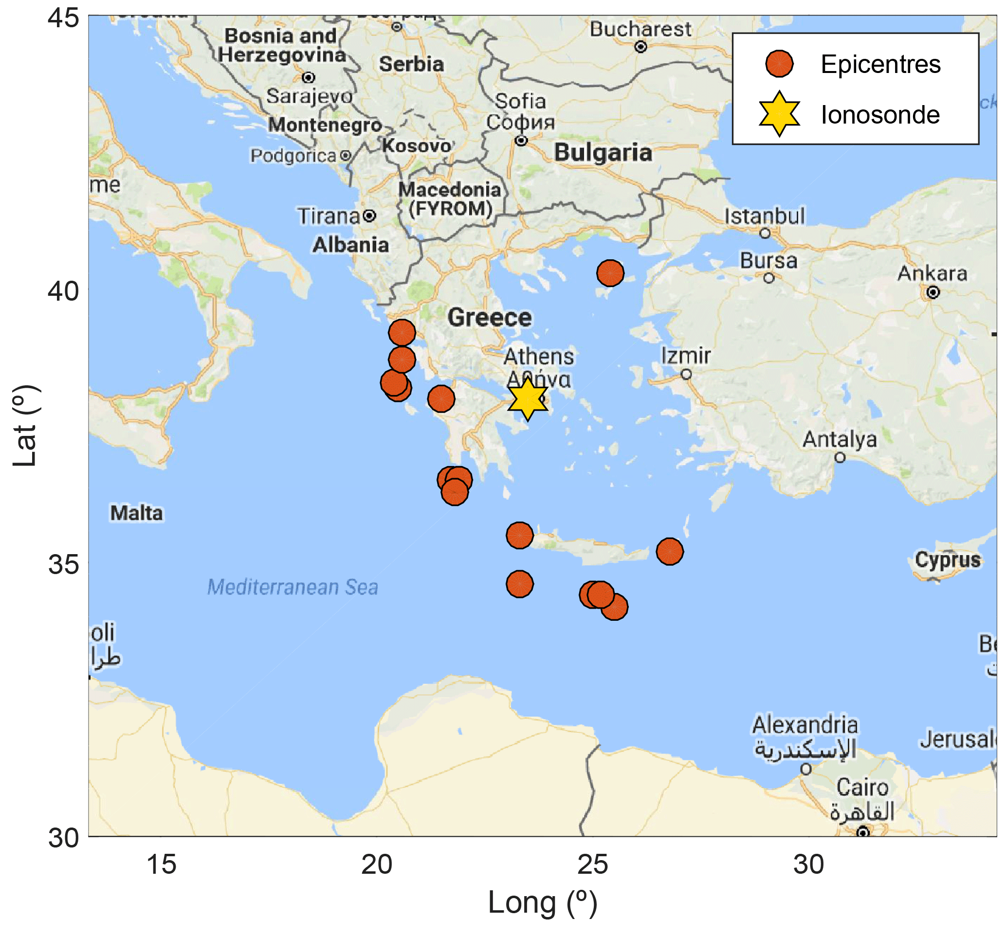
Figure 1 Epicentres of major earthquakes in Greece and surrounding area (M≥6, depth <50 km) between January 2003 and December 2015 and the ionosonde location.

Table 1 List of the shallow earthquakes (hypocentral depth <50 km) with magnitude M≥6.0 registered in Greece during 2003–2015. Geographical coordinates of the earthquake epicentres (from United States Geological Survey USGS, 2017) and the distance (R) from the Athens ionosonde are also given. EQs with (∗) have not been analysed because are too distant from the Athens ionosonde station (R>350 km).

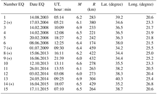
Table 1 also shows the distance R from the ionosonde station to the epicentre calculated along the great cycle path. The correction of R when such distance is propagated to the E-region heights is <2 km for the selected events and it can be ignored. The epicentres are located at a distance 90–500 km from Athens.

However, it was found that there is a limitation in distance after which we could not find any reliable ionospheric anomalies (Korsunova and Khegai, 2008; Perrone et al., 2010). In our case, we did not analyse the more distant EQs from the Athens ionosonde station, i.e. those with R>350 km (EQs indicated by an asterisk in Table 1). Therefore the case studies analysed were reduced to 10 EQs.

It should be stressed that the analysis of the EQ ionospheric anomalies in the nearest ionosonde to the epicentre zone is most important from a practical point of view. In the next paragraph, we will explain the procedure.

According to Korsunova and Khegai (2008) and Perrone et al. (2010), the deviations in h^′Es, fbEs and foF2 ionospheric parameters should simultaneously satisfy the ionospheric anomaly selection criteria.

Unfortunately, the fbEs parameter is obtained by manual scaling of the ionograms and currently very few ionospheric observatories provide such a parameter. In such cases, instead of using the fbEs parameter, we use foEs, which is scaled automatically.

The occurrence of abnormally high Es layer for 2–3 h is considered necessary to identify anomalies. The h^′Es height should exceed the corresponding background values by ≥10 km. An increase in foEs and foF2 also for 2–3 h during the same day soon after the h^′Es increase is considered sufficient to identify ionospheric anomalies. The critical frequency foEs excess over the background value should be not less than 20 %. Electron concentration in the F2 layer is subjected to large and irregular variations; however, an increase in foF2 by ≥10 % over the background level also for 2–3 h after the increases in h^′Es and foEs should take place.

Ionospheric data analysis comprises some steps.

First, the background h^′Es, foEs, foF2 variations are specified. They characterize quiet-time diurnal variations for the years and months analysed. The 27-day running medians calculated over all quiet (Ap ≤15) days are used as the background values. Then, absolute $\mathrm{\Delta }{\mathrm{h}}^{\prime }\text{Es}={\mathrm{h}}^{\prime }\text{Es}-({\mathrm{h}}^{\prime }\text{Es}{)}_{\text{med}}$, $\mathrm{\Delta }\mathit{fo}\text{Es}=\mathit{fo}\text{Es}-(\mathit{fo}\text{Es}{)}_{\text{med}}$, Δ foF2 = foF2 − (foF2)_med and relative ΔfoEs∕(foEs)_med, ΔfoF2∕(foF2)_med deviations are calculated for every hour of each day. Finally, we look for the ionospheric anomaly in the 4 months preceding the earthquake. Middle-term earthquake precursors may occur some months in advance (Korsunova and Khegai, 2006; Hao et al., 2000).

Particular attention in the data analysis has to be paid to the fact that the coupling of the ionosphere with the magnetosphere makes the former highly sensitive to the variations of the external field modulated by the solar activity, masking other effects such as the coupling with the lithosphere we are investigate here. Specifically, while the magnetosphere is influenced by the solar wind parameters and by the strength and orientation of the interplanetary magnetic field (IMF), the ionospheric behaviour is principally modulated by the level of solar and geomagnetic activity (Cander, 2016). The ionospheric parameters are variable and affected from above (solar extreme ultraviolet, EUV; magnetospheric and dynamo electric fields; changing thermospheric circulation and neutral composition; travelling atmospheric disturbances, TADs; etc.) and from below (planetary and gravity waves, neutral gas vertical motion and eddy diffusion changing thermospheric neutral composition, tropospheric electric fields not necessarily related to seismic processes). This leads to the fact that ionospheric behaviour is hard to predict, in terms of occurrence and determination of the causes behind the formation of the ionospheric irregularities in space and time.

Thus, we have to exclude ionospheric anomalies that could originate from external forcing. To this aim, detailed information about the physical state of the entire Sun–Earth system is required and, consequently, several geophysical indices are monitored. Two geomagnetic indices have been used in this analysis to characterize the geomagnetic activity:

• ap index: a 3 h index, available since 1932. It is expressed in nanotesla and derived from another index, the Kp, which is an almost logarithmic scale with respect to the field variations and it is based on the geomagnetic field data from 11 observatories located at mid- and high latitudes. This index is commonly used in ionospheric studies, especially in ionospheric forecasting models and long-term studies (Perrone and De Franceschi, 1998). In this work, we considered the Ap index that is the daily average of the corresponding eight ap values of the day (ftp://ftp.ngdc.noaa.gov/STP/GEOMAGNETIC_DATA/INDICES/KP_AP).

• AE index: a 1 min index, available since 1957. It is computed using a network of auroral observatories and it is introduced to characterize the auroral zone, where the fluctuations of the magnetic field are much stronger than at mid- and low latitudes. In the ionospheric studies, it is used to check if local ionospheric variations are due to an increase in auroral activity that could influence the mid- and low-latitude ionosphere (Perrone and De Franceschi, 1998). In this work, we considered the 1 h mean of AE (http://wdc.kugi.kyoto-u.ac.jp/aedir/).

In this study, the ionospheric anomaly associated with an earthquake must occur under magnetically quiet conditions, which are defined as

1. Daily geomagnetic index Ap ≤15.

2. The auroral electrojet index AE: in summer and equinox this should be ≤100 nT and in winter ≤200 nT for the previous 6 h. Different limits applied to AE index are due to different meridional thermospheric circulation in different seasons. Meridional daytime wind at middle latitudes is mainly equatorward in summer and equinox, easing the perturbation to penetrate from the auroral zone to middle latitudes, while in winter the meridional circulation during daytime is mostly poleward, constraining the perturbation at high latitudes (Buonsanto and Witasse, 1999; Prölss and von Zahn, 1977; Prölss, 1993; Field et al., 1998).

We considered 6 h before the occurrence of an ionospheric anomaly because TADs related to upsurges of auroral activity can reach middle latitudes and perturb foF2. Under the average TAD velocity at F2-region heights of 500–600 m s⁻¹ (Bruinsma and Forbes, 2010; Mikhailov and Perrone, 2009; Mikhailov et al., 2012), the arrival of a TAD at middle latitudes is expected in 2–3 h.

Sometimes EQs follow each other with a small time interval (see 3a, 3b in Table 1), and it may be problematic to correlate a particular ionospheric anomaly with a single, corresponding earthquake. In such cases, the following rule is used: under approximately equal epicentre distances, an ionospheric anomaly for an earthquake with larger magnitude occurs earlier and produces larger deviations in h^′Es (Korsunova and Khegai, 2006).

Table 2 gives the ionospheric anomalies found with the corresponding parameters and the related earthquakes.

Table 2 Identified ionospheric anomalies and corresponding EQs (the EQ order no. is the same used in Table 1). Daily Ap indices are given as well.

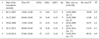
For the EQ that took place on 8 June 2008 (EQ no. 6, Table 1), no ionospheric anomalies were found. For the other remaining four EQs, nos. 1, 10, 12 and 15, the ionospheric anomalies were found but they did not occur during quiet magnetic conditions (see criteria 1 and 2 given earlier).

As an example of valid pre-EQ anomaly, Δh^′Es, δfoEs and δfoF2 variations along with 3 h a_p for the EQ occurred on 24 May 2014 (EQ no. 13) are given in Fig. 2.

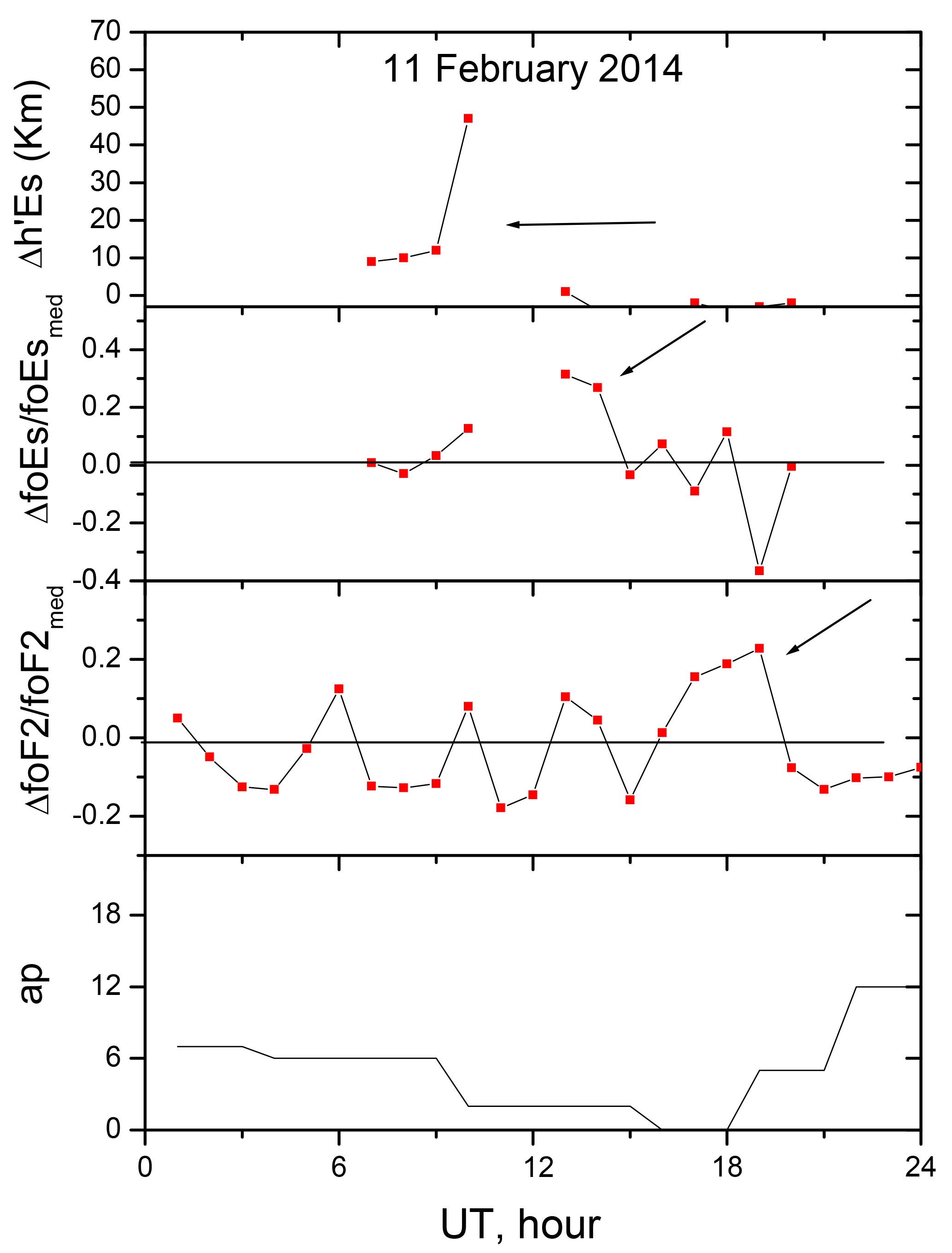
Figure 2 The ionospheric anomaly for the 24.05.14 EQ using observed Δh^′Es, δfoEs and δfoF2 variations (arrows). Three-hour a_p indices are given in lower panel.

3 Results

The applied method uses three ionospheric ionosonde parameters simultaneously: 2–3 h splashes in Δh^′Es, δfoEs and δfoF2 above the corresponding thresholds should take place within 1 day.

There are relationships for middle-term ionospheric anomalies related to lead time ΔT, which is the time in advance between the ionospheric anomaly and the EQ occurrence, with the EQ magnitude M and the epicentre distance R (Sidorin, 1992; Korsunova and Khegai, 2006; Perrone et al., 2010).

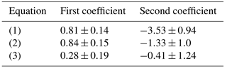
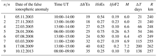
Such relationships are given in Fig. 3 (black squares) for the events listed in Table 2. The upper panel gives the dependence for (the decimal logarithm of) lead time on the EQ magnitude. The middle panel gives the same dependence, but for the product (ΔT×R), while the lower panel gives the dependence for Δh^′Es on the earthquake magnitude M. The dependencies are statistically significant at the 99 % level for the first two relationships and at the 97.5 % for the third confidence level, according to Fisher criterion.

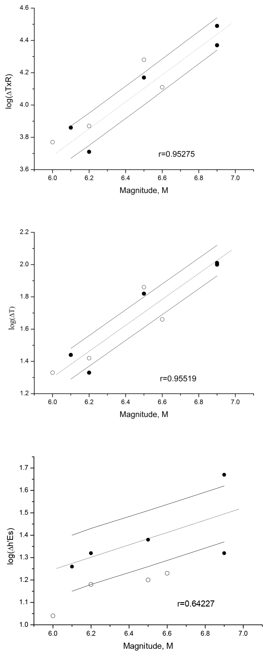
Figure 3 The observed dependencies for (from top to bottom) log (ΔT×R), log ΔT and log (Δ h^′Es) on the EQ magnitude. Correlation coefficients (r) of the points from the regression line are given. Each dash line is the best linear fit, while the continuous lines are those corresponding to ± 1 standard deviation (SD).

The relationships obtained for log (ΔT), log (ΔT×R) and log (Δh^′Es) are

$$\begin{array}{}\text{(1)}& {\displaystyle }& {\displaystyle }\log \left(\mathrm{\Delta }T\right)=\mathrm{0.81}M-\mathrm{3.53};\text{(2)}& {\displaystyle }& {\displaystyle }\log (\mathrm{\Delta }T\times R)=\mathrm{0.84}M-\mathrm{1.33};\text{(3)}& {\displaystyle }& {\displaystyle }\log \left(\mathrm{\Delta }{\mathrm{h}}^{\prime }\text{Es}\right)=\mathrm{0.28}M-\mathrm{0.41}.\end{array}$$

The standard errors associated with the regressions (1–3) coefficients are given in Table 3.

Table 3 Coefficients of the regressions (1–3) and their standard errors.

Due to the small statistics size (only five events), the uncertainty in the coefficients is rather large. However, the relationships obtained are similar to those obtained in previous research. In particular, Korsunova and Khegai (2006), for 33 powerful earthquakes with M≥6 that occurred in the region of Kokubunji station in 1985–2000, obtained the following relationship:

$$\begin{array}{}\text{(4)}& \log \left(\mathrm{\Delta }T\times R\right)=\mathrm{1.14}M-\mathrm{4.72}\end{array}$$

Perrone et al. (2010) for moderate central Italian earthquakes obtained the following.

$$\begin{array}{}\text{(5)}& {\displaystyle }& {\displaystyle }\log \left(\mathrm{\Delta }T\right)=\mathrm{1.09}M-\mathrm{4.897}\text{(6)}& {\displaystyle }& {\displaystyle }\log \left(\mathrm{\Delta }T\times R\right)=\mathrm{0.886}M-\mathrm{1.626}\text{(7)}& {\displaystyle }& {\displaystyle }\log \left(\mathrm{\Delta }{\mathrm{h}}^{\prime }\text{Es}\right)=\mathrm{0.672}M-\mathrm{2.422}\end{array}$$

Ground observations of various geophysical parameters for a number of earthquakes with magnitude in the range 4–8 (Sidorin, 1992) resulted in the following dependence.

$$\begin{array}{}\text{(8)}& \log \left(\mathrm{\Delta }T\times R\right)=\mathrm{0.72}M-\mathrm{0.72}\end{array}$$

A qualitative agreement is seen for Eqs. (1)–(6), obtained using both ground and ionospheric precursors. The similarity of the relationships that were obtained in different parts of the world seems to confirm the uniformity of the solid earth and ionosphere coupling processes during the EQ preparation period.

Another aspect of earthquake prediction is the number of false cases in the same period of study, i.e. all years from 2003 to 2015. For this purpose, the Δh^′Es, δfoEs and δfoF2 deviations were calculated for every hour of all days and all months of these years. The calculated values were then analysed for ionospheric anomalies in accordance with our criteria. The list of all false cases, i.e. those cases for which we revealed the ionospheric anomalies during quiet magnetic conditions according to our criteria but no EQs occurred, is given in Table 4 along with M, ΔT, and R values calculated using the relationships (1–3). We have not listed the ionospheric anomalies from which we obtained these empirical relationships (Table 2).

Table 4 Revealed false ionospheric anomalies for quiet periods between 2003 and 2015 along with calculated M, ΔT, R values using the relationships (1–3). Only expected events with M≥6.0 are listed.

Only the characteristics of strong (M≥6.0) expected events are listed in Table 4. The analysis undertaken has shown that false cases do exist in the years analysed. They are not found to be numerous, but their number is comparable to the number of real earthquakes (Table 2) and they are not distinguished from the previous ionospheric anomalies (Table 2).

4 Forecast possibilities of the method

An important result of our analysis is the provision of quantitative expressions (1–3) relating the EQ magnitude and the epicentre distance with observed h^′Es variations for the Greek region. In principle, such expressions could be used for prediction purposes to determine the magnitude M and lead time ΔT of a future earthquake.

However, large uncertainty (due to small statistics) of the regression coefficients (Table 3) does not allow us to make such a prediction with acceptable accuracy.

Dependences similar to (1–3) would only make practical sense if the probability of false cases is not high. A special analysis has been undertaken to clarify this question.

4.1 Confusion matrix

Receiver operating characteristic (ROC) analysis has been performed in terms of a confusion matrix, giving the discrete joint sample distribution of forecasts and observations in terms of cell counts (e.g. Fawcett, 2006). It is very useful to perform an objective validation of the method and a comparison with respect to a random system.

We checked our ionospheric anomalies 4 months before all EQ occurrences so we could see if a possible precursory anomaly could exist in a cell of 4 months. For dichotomous categorical forecasts, having only two possible outcomes (yes or no), the (2×2) confusion matrix of Table 5 can be defined.

The parameters indicated in Table 5 are the following:

• a is the number of the ionospheric anomalies followed by an earthquake: true cases;

• b is the number of ionospheric anomalies that do not correspond to earthquakes: the number of false alarms;

• d is the number of cases where there were no ionospheric anomalies followed by an earthquake: the number of misses;

• c is the number of forecasts with no events corresponding to no events observed: the number of correct rejections.

Table 5 Confusion matrix.

Forecast quality for this (2×2) binary situation can be assessed using a surprisingly large number of different measures, detailed in the following.

The hit rate (H) is the number of EQs preceded by an anomaly, so it is an indication of the predictability of the events: the closer to 1, the better the value. In our case, $H=\frac{a}{a+d}=\frac{\mathrm{5}}{\mathrm{10}}=\mathrm{0.5}$.

The false alarms (F) are the number of anomalies without a following earthquake: the closer to 0, the better the value. In our case, $F=\frac{b}{b+c}=\frac{\mathrm{9}}{\mathrm{35}}=\mathrm{0.26}$. In some cases, the false alarm could be due to a non-seismic source responsible for the ionospheric anomaly. It is possible to reduce the number of false alarms using other observables in a multi-parametric integrated approach (e.g. De Santis et al., 2015).

Obviously, the best method provides both a high H and a low F. A non-optimal case would be for alarms every time before impending earthquakes but at the price of an increased amount of false alarms, and so the prediction system fails.

The accuracy, Acc, which is given by $(a+c)/e$, is a global evaluation of the method and is a comparison of the success (anomaly + earthquake or no anomaly + no seismic activity) with respect to the total number of cases analysed. The closer its value to 1, the better the method. In our case, $\text{Acc}=\frac{a+c}{e}=\frac{\mathrm{25}}{\mathrm{39}}=\mathrm{0.69}$.

Gain, G, and R score (e.g. Aki, 1981) are some evaluation quality factors that are an indication of the improvement of the method with respect to a random system. The more positive the G, the better the method. The R score can assume real (positive, null or negative) values. If R score is negative the method is worse than a random system; R score =0 means that the method behaves as a random guess; a positive value means that the method is better than a random system. R score equal to −1 is a total fail, while R score equal to 1 is a perfect (ideal) method of prediction.

$$G=h\times \left({\displaystyle \frac{e}{a+b}}\right)=\mathrm{1.61}$$

The R score can be evaluated in two ways:

$$\begin{array}{ll}{\displaystyle }& {\displaystyle }R={\displaystyle \frac{a}{a+b}}-{\displaystyle \frac{d}{c+d}}=\mathrm{0.2},\\ {\displaystyle }& {\displaystyle }{R}^{\prime }=H-F=\mathrm{0.24}.\end{array}$$

The accuracy is near 70 %, although the hit rate is not above 50 %, and the false alarm rate is 26 %. R score is positive, indicating a good forecast method.

The global evaluation of the method by these factors is quite positive. The results provided by the method of EQ forecast based on ionosonde data are clearly better than a random guess system.

4.2 Ionospheric anomalies during an increase in auroral activity

It is interesting to note that even some of the ionospheric anomalies that have been previously discarded because of the stringent limits imposed by the magnetic indices could have some forecast value. Figure 4 gives, together with the previous validated ionospheric anomalies, also those (empty squares) with Ap <20, but with an AE larger than the imposed limits, which could be linked to the other four EQs (Table 6). Details on these discarded cases are given in Table 6, but it should be stressed that the number of ionospheric anomalies not related to earthquakes increases during a disturbed period: from 2003 to 2015, we find 36 of this type of ionospheric anomaly, and only 4 of them could be related to earthquakes.

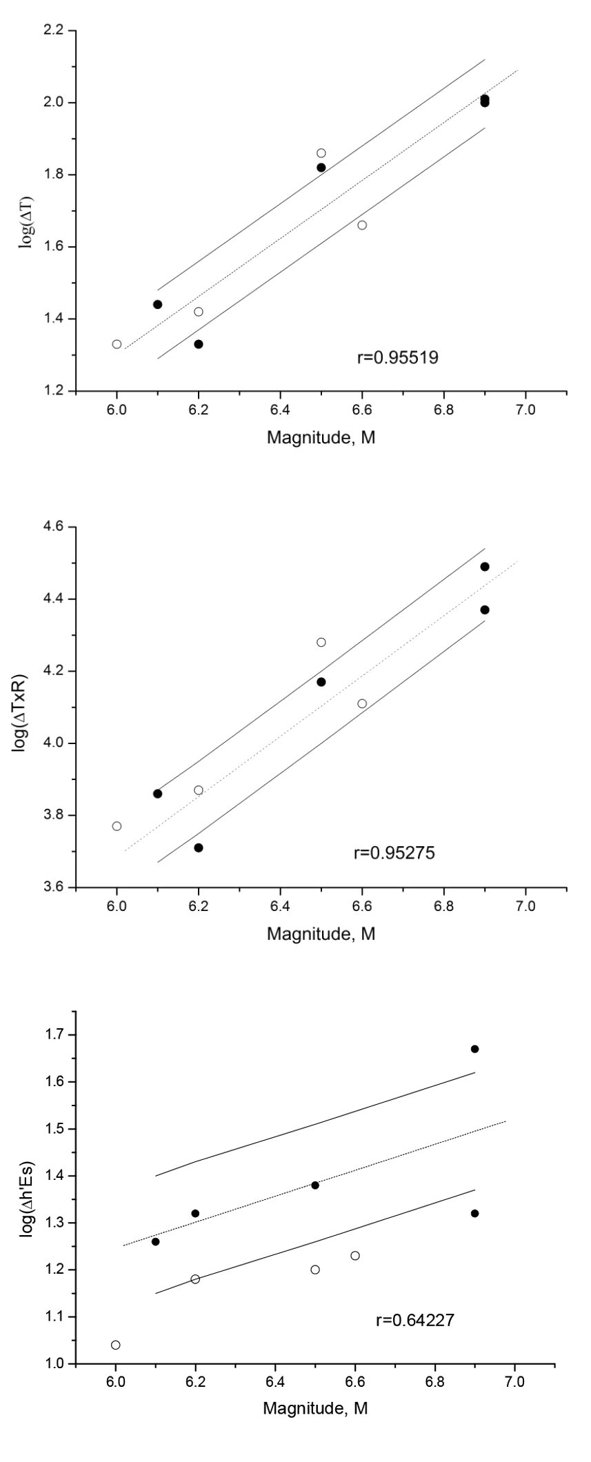
Figure 4 The observed dependencies for log (ΔT), log (ΔT×R) and log (Δh^′Es) on the EQ magnitude. Correlation coefficients (r) of the points from the regression line are given. Each dash line is the best linear fit, while the continuous lines are those corresponding to ± 1 standard deviation (SD). Empty squares represent those discarded anomalies characterized by an AE larger than the imposed limits.

Table 6 Revealed ionospheric anomalies during disturbed magnetic conditions (AE larger than the imposed limits) and corresponding earthquakes, daily Ap indices are given as well.

5 Discussion

The analysis undertaken has shown that the approach proposed by Korsunova and Khegai (2006, 2008) and Perrone et al. (2010) can be applied to earthquakes with M>6.0 taking place in Greece in the vicinity of Athens (i.e. well within the Dobrovolsky strain radius ρ). The simultaneous deviations in Δh^′Es, δfoEs and δfoF2 above the corresponding thresholds for 2–3 h following each other within 1 day can be related by logarithmic dependences with the EQ magnitude and the epicentre distance. Despite the few available cases, the dependences obtained (1–3) for log (ΔT), log (ΔT×R) and log (Δh^′Es) vs. the EQ magnitude are statistically significant at the 99 % confidence level.

A theory of the earthquake preparation taking into account the electromagnetic processes in the lithosphere–atmosphere–ionosphere system (e.g. Kim et al., 1994; Pulinets et al., 1998; Sorokin et al., 2006) suggests the formation of a sporadic E layer with large electron concentration at the heights of 120–140 km above the earthquake preparation zone. Long-living (Δt≈2–3 h), sporadic Es layers revealed and used in our analysis occur at heights of ≥10 km higher than normal Es for corresponding geophysical conditions. Their formation is accompanied by an increase in foEs and foF2.

In this work, we demonstrate that the method previously applied to Japanese and central Italian EQs is also valid for Greek EQs. The ionospheric anomalies found with the Athens ionosonde can be considered middle-term seismic precursors.

Our method to identify ionospheric anomalies uses three parameters simultaneously (Δh^′Es being the main parameter), and this is the principal difference with other methods based on just one ionospheric parameter, for instance, foF2 (e.g. Liu et al., 2006; Dabas et al., 2007). Although the authors attempted to avoid periods with higher geomagnetic activity in their analyses, foF2 is a very variable parameter, affected both from above (e.g. by solar EUV, magnetospheric and dynamo electric fields, changing thermospheric circulation and neutral composition, TADs etc.; Bremer et al., 2009; Kutiev et al., 2013; Mikhailov and Perrone, 2015) and from below (e.g. planetary and gravity waves, neutral gas vertical motion and eddy diffusion changing thermospheric neutral composition, tropospheric electric fields not necessary related to seismic processes). Therefore, besides the geomagnetic activity effects, there are many other sources of foF2 variations. The morphology of the F2-layer perturbations not related to geomagnetic activity (so-called Q-disturbances) can be found in Mikhailov et al. (2004) and Depueva et al. (2005). The equatorial and low-latitude F2 region considered by Dabas et al. (2007) is strongly affected by electric fields, which exhibit large variability even under geomagnetically quiet conditions (e.g. counter electrojet). Therefore, foF2 is a very “inconvenient” ionospheric parameter for the role of an earthquake precursor, if used alone without other parameters. For this reason, in our method foF2 is considered to be a parameter whose variations are taken into account only along with Es parameter variations, but 2–3 h deviations in ΔfoF2 above the background level should take place as well.

In this paper, along with daily Ap, we have used an additional geomagnetic activity index of auroral activity, AE, to define quiet geomagnetic conditions. This was used because upsurges of auroral activity can launch TADs which might perturb mid-latitude F2 layer, without be reflected in the anomalous daily Ap index.

We conclude with some words concerning the possibility of using this method in an operational environment to find reliable earthquake precursors. We have shown that the statistical reliability of the regression coefficients is not very high and prevents us from making any quantitative forecasts. Another problem of real forecast is the non-zero probability of false alarms: although they are not numerous (Tables 4 and 5), they exhibit the same features as the real ones so they cannot be distinguished in any real time prediction scheme.

On the other hand, our method can be used as an independent and original contribution within a more integrated system of earthquake prediction, where many other EQ-sensitive physical parameters are considered as well (e.g. De Santis et al., 2015).

6 Conclusions

The results of our analysis may be summarized as follows.

The method earlier used for Japanese and central Italian earthquakes (Korsunova and Khegay, 2008, and Perrone et al., 2010, respectively) was shown to be applicable also for M≥6 Greek earthquakes. It is based on observed simultaneous deviations in Δh^′Es, δfoEs∕δfbEs and δfoF2 above the corresponding thresholds for 2–3 h following each other within 1 day. An observed set of such deviations in the ionospheric parameters is considered to be a middle-term ionospheric anomaly.

The ionospheric anomalies that occur during a period of increased auroral activity (i.e. with high values of AE index) should not be considered in the analysis: this reduces the possibility of contaminating the results with external sources. However, we have also showed that some of them could be potential EQ precursors, but before extending the analysis to increased auroral activity periods, more investigation is needed.

The observed ionospheric anomalies resulted in the relationship relating the lead time ΔT with the earthquake magnitude M and the epicentre distance R. The relationship obtained is statistically significant at the 99 % confidence level and it looks similar to those obtained earlier for Japanese and central Italian earthquakes. The relationship indicates the process of spreading the disturbance from the epicentre towards periphery during the earthquake preparation process (Perrone et al., 2010).

There are ionospheric anomalies not related to earthquakes. They are not numerous but they are comparable with those potentially associated with the seismic events and, even more importantly, they cannot be uniquely distinguished from the ionospheric anomalies linked to the earthquakes.

A systematic statistical analysis of 13 years of ionosonde data from the Athens station has been undertaken, and the final result is that the method has great potential for use in EQ prediction, especially when it is integrated with other appropriate independent data (De Santis et al., 2015).