the Creative Commons Attribution 4.0 License.
the Creative Commons Attribution 4.0 License.
 | 27 Jul 2018
A possible source mechanism for magnetotail current sheet flapping
Yann Pfau-Kempf
Urs Ganse
Markus Battarbee
Thiago Brito
Maxime Grandin
Lucile Turc
Minna Palmroth
The origin of the flapping motions of the current sheet in the Earth's magnetotail is one of the most interesting questions of magnetospheric dynamics yet to be solved. We have used a polar plane simulation from the global hybrid-Vlasov model Vlasiator to study the characteristics and source of current sheet flapping in the center of the magnetotail. The characteristics of the simulated signatures agree with observations reported in the literature. The flapping is initiated by a hemispherically asymmetric magnetopause perturbation, created by subsolar magnetopause reconnection, that is capable of displacing the tail current sheet from its nominal position. The current sheet displacement propagates downtail at the same pace as the driving magnetopause perturbation. The initial current sheet displacement launches a standing magnetosonic wave within the tail resonance cavity. The travel time of the wave within the local cavity determines the period of the subsequent flapping signatures. Compression of the tail lobes due to added flux affects the cross-sectional width of the resonance cavity as well as the magnetosonic speed within the cavity. These in turn modify the wave travel time and flapping period. The compression of the resonance cavity may also provide additional energy to the standing wave, which may lead to strengthening of the flapping signature. It may be possible that the suggested mechanism could act as a source of kink-like waves that have been observed to be emitted from the center of the tail and to propagate toward the dawn and dusk flanks.
- Article
(20490 KB) - Full-text XML
- BibTeX
- EndNote


The magnetotail current or neutral sheet is a relatively narrow region of lobe magnetic field reversal within a broader plasma sheet region between the tail lobes. A satellite on an orbit passing through this region often observes multiple current sheet crossings, indicating that the sheet moves up and down relative to the spacecraft several times. This flapping motion of the current sheet is observed as up to tens of nT variations in the magnetic field geocentric solar magnetospheric (GSM) Bx component, often associated with a change in polarity of Bx (Speiser and Ness, 1967).
The temporal scale of the flapping variations ranges from tens of seconds to tens of minutes (Sergeev et al., 1998). The variations are interpreted as up and down motion of the current sheet with respect to the stationary satellite, such that anticorrelates with the GSM north component of the plasma bulk velocity (Vz). Sergeev et al. (1998) show example events with Vz varying from some tens of km s−1 to some hundreds of km s−1. The majority of the flapping events are observed during thin current sheets within ±10 min around substorm onset or intensification (Sergeev et al., 1998). Laitinen et al. (2007) presented an event during which current sheet oscillations were timed to occur both before tail reconnection and during it.
Two types of flapping motions have been distinguished: steady flapping and kink-like flapping (Rong et al., 2015). Steady flapping refers to oscillations in the z direction during which the current sheet normal remains more or less in the same direction. Such oscillations do not propagate as waves but remain stationary. The kink-like flapping, on the other hand, is able to propagate as waves. The sheet as a whole is tilted, rather than being locally expanded and contracted like in the sausage wave, which could also have explained the observed flapping signatures (Runov et al., 2003; Sergeev et al., 2003). The kink-like flapping may propagate along the y axis, in which case the current sheet normals for subsequent crossings vary in the y−z plane, or along the x axis, so that the normals vary in the x−z plane (Rong et al., 2015; Sun et al., 2013). All three flapping types (steady flapping, kink-like along y, and kink-like along x) can yield similar time series of the Bx component.
Flapping has been observed as close to the Earth as 12 Earth radii (RE), i.e., close to the transition region or hinge point between tail-like and dipolar field lines (Sergeev et al., 1998). The waves are tail-aligned structures with the cross-tail wavelength (∼5 RE) clearly smaller than the along-tail length (>10 RE) (Runov et al., 2009), and are observed to propagate toward the flanks from the center of the tail at velocities of some tens of km s−1 (Sergeev et al., 2004).
The origin of the flapping motion has not been established, although several tentative explanations, including solar wind variations (Forsyth et al., 2009; Sergeev et al., 2008; Shen et al., 2008; Speiser and Ness, 1967) and internal sources (Davey et al., 2012; Golovchanskaya and Maltsev, 2005; Sergeev et al., 2004; Wei et al., 2015; Zelenyi et al., 2009), have been suggested. Bursty bulk flows (BBFs), produced as outflows from tail reconnection, are among the suggested internal sources (Erkaev et al., 2009; Gabrielse et al., 2008). Statistical results have demonstrated that the occurrence rate of flapping motions is similar to that of BBFs, and peak in the central part of the magnetotail (Sergeev et al., 2006). Empirical models (Petrukovich et al., 2008; Rong et al., 2010) have been constructed to describe the characteristics of flapping current sheets.
In this study, we analyze a two-dimensional (2-D) polar plane simulation produced using the global magnetospheric hybrid-Vlasov model Vlasiator1. The simulation is driven by steady solar wind, characterized by high solar wind speed and a southward interplanetary magnetic field (IMF). About half an hour after the start of the simulation, tail reconnection begins. The same run has been used earlier to analyze subsolar magnetopause reconnection (Hoilijoki et al., 2017), onset of tail reconnection (Palmroth et al., 2017), and ion acceleration by flux transfer events in the magnetosheath (Jarvinen et al., 2018). Our aim is to examine the current sheet flapping signatures present in the simulation before and after the onset of tail reconnection, and to determine the driver of the flapping motions. Because the simulation is 2-D, we concentrate on the characteristics and source of the waves in the center of the tail (i.e., waves in the x−z plane). We also discuss to possibility that in 3-D, they could drive the kink-like waves that are emitted from the center of the tail and propagate dawnward and duskward (i.e., waves in the y−z plane). The structure of the paper is as follows: the Vlasiator model is described in Sect. 2 and the results presented in Sect. 3. Section 4 contains discussion and Sect. 5 summarizes the conclusions.
We use the hybrid-Vlasov model Vlasiator (Palmroth et al., 2013, 2015; von Alfthan et al., 2014). In this version of the simulation, ions are modeled as 5-D velocity distribution functions (2-D in space, 3-D in velocity) that are propagated in time according to Vlasov's equation. Ampère's law, Faraday's law, and generalized Ohm's law, including the Hall term, complete the set of equations. Electrons are neglected apart from their charge-neutralizing behavior.
The spatial resolution of the 2-D polar plane simulation is km or ∼0.047 RE (1 RE=6371 km) and the velocity space resolution km s−1. The velocity space in each spatial grid cell covers km s−1. The simulation box extends from x=300 000 km or ∼47 RE on the dayside to 000 km or RE on the nightside. In the north–south direction the box covers 000 km or RE. The inner boundary of the simulation is at the distance of 30 000 km or ∼5 RE from the origin. The geomagnetic field is modeled as a 2-D line dipole that is centered at the origin, aligned with the z axis, and scaled to result in a realistic magnetopause standoff distance (Daldorff et al., 2014). Thus, the coordinate system is comparable to GSM.
Steady solar wind, characterized by Maxwellian distribution functions, proton density of 1 cm−3, temperature of 0.5 MK, velocity of −750 km s−1 along the x axis, and magnetic field of −5 nT along the z axis (purely southward IMF), is fed into the simulation box from its sunward wall (+x). Copy conditions are applied to the other outer walls (−x, ±z), and periodic boundary conditions to the out-of-plane (±y) directions. The inner boundary enforces a static Maxwellian velocity distribution and perfect conductor field boundary conditions. The simulation output (moments and fields) is saved every simulated 0.5 s.
In this section, we start (Sect. 3.1) by examining the characteristics of the current sheet flapping signatures in the simulation and by comparing them with the observations cited in the Introduction. After that (Sect. 3.2), we suggest a mechanism that could explain how the flapping motion is initiated and maintained.
Figure 1 introduces the x−z plane simulation by showing a snapshot at 19 min and 40 s after the start of the run. The background color displays the ratio of the ion thermal pressure perpendicular to the magnetic field and the magnetic pressure (). Closed magnetic field lines are drawn as green curves, semi-open field lines (with one footpoint at the inner boundary) as black curves, and open field lines as gray curves. Field lines that are closed but not attached to the geomagnetic field are drawn in magenta. The tail lobes are estimated to lie between the blue curves. These curves indicate the innermost boundaries where in the region RE and x<0. This proxy is based on the assumption that while the magnetosheath is dominated by the plasma pressure, the tail lobes are magnetically dominated. At the time shown, a hemispherically asymmetric magnetopause perturbation, created around the time when subsolar reconnection first started to add new semi-open flux tubes to the lobes, has reached the distance RE (inside the red box). The significance of this perturbation will be discussed further in Sect. 3.2.
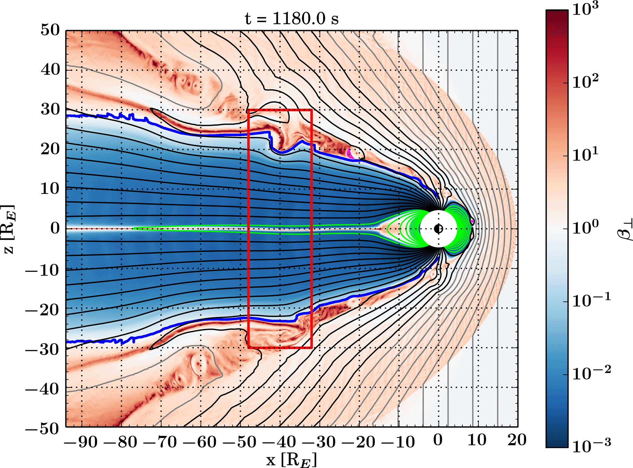
Figure 1Ratio of ion thermal pressure perpendicular to the magnetic field and magnetic pressure and magnetic field lines in the x−z plane at 19:40 (1180.0 s). Closed field lines are drawn in green, semi-open field lines in black, and open field lines in gray. Field lines that are closed but not attached to the geomagnetic field are drawn in magenta. The tail lobes are estimated to lie between the blue curves. The curves indicate the innermost boundaries where in the region RE and x<0. Inside the red box, a hemispherically asymmetric magnetopause perturbation compresses the northern tail lobe and expands the southern tail lobe, causing the current sheet between the tail lobes around RE to shift slightly southward from its nominal position at z=0.
3.1 Characteristics of current sheet flapping signatures
Figure 2 shows the earthward component of the magnetic field (Bx, color) at the nominal location of the magnetotail current sheet () as a function of x and time (MM:SS, where MM indicates minutes and SS seconds). The tilted black lines indicate motion at the solar wind velocity km s−1. The vertical black lines at 19:40 and 27:00 mark the time of Fig. 1 and the onset time of tail reconnection at RE (Palmroth et al., 2017), respectively. The most striking feature in the plot is the alternating positive and negative enhancements of Bx on the order of 10 nT in amplitude. The signatures first appear in the transition region and subsequently propagate tailward at a velocity which is generally close to the solar wind velocity as indicated by the tilted black lines. The Bx enhancements can appear to be fairly regular for a while (e.g., around RE between 24:00 and 30:00) or quite irregular (e.g., tailward of RE). The durations of the enhancements at a given location vary from a few minutes to less than a minute, in agreement with Sergeev et al. (1998). The along-tail lengths of the signatures vary, but can be >10 RE, in agreement with Runov et al. (2009). The enhancements occur for ∼13 min before the onset of tail reconnection as indicated by the vertical black line, and can be observed at least for ∼4 min after, in agreement with Sergeev et al. (1998) and Laitinen et al. (2007), before the signatures are disrupted by the spreading effects of tail reconnection. After this, Bx enhancements can still be observed between −30 and −10 RE until the end of the simulation, i.e., 9 min after the onset of reconnection.

Figure 2Earthward component of the magnetic field (Bx, color) at the nominal position of the tail current sheet () as a function of x and time (MM:SS, where MM indicates minutes and SS seconds). The tilted black lines indicate motion at the solar wind velocity km s−1. The vertical black lines at 19:40 and 27:00 mark the time of Fig. 1 and the onset time of tail reconnection at RE, respectively.
The Bx signatures resemble those associated with current sheet flapping, discussed in the Introduction. In order to check whether this might indeed be the case, Fig. 3 shows the time derivative of Bx () and Fig. 4 the z component of the ion bulk velocity (Vz). The cyan curves in Fig. 4 indicate isocontours of pressure in the z direction () with a thicker curve indicating higher pressure (levels 0.05, 0.1 , and 0.2 nPa). The curves have only been plotted in the tail-like region undisturbed by significant effects from tail reconnection. The magenta dots in Fig. 4 mark flapping half periods at RE, RE, and RE, identified based on sign changes of Vz. Comparison of Fig. 3 and Fig. 4 shows that Vz and are anticorrelated (this can also be seen in Fig. 7 below), implying that the variations in Bx are caused by up and down motion of the current sheet with respect to the z=0 plane (Sergeev et al., 1998). The amplitude of Vz is also in agreement with the observations of Sergeev et al. (1998).
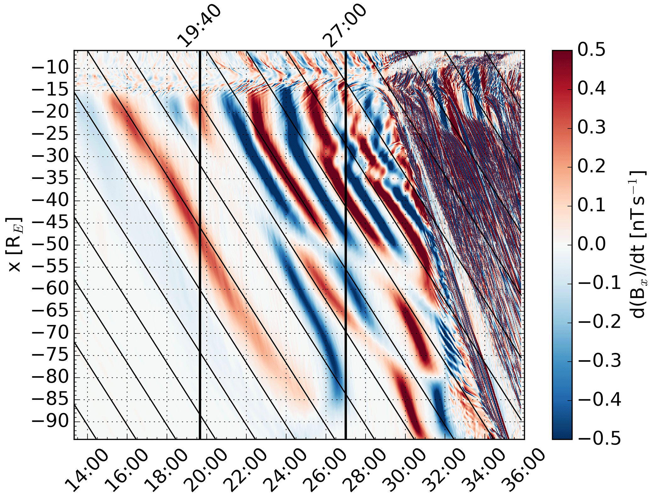
Figure 3The same as Fig. 2 except that the color shows the time derivative of Bx. The color scale has been saturated to better show the relevant structures.
Figure 4 illustrates that while the first significant signature of downward ion bulk flow (blue) propagates all the way through the tail at a speed very close to the solar wind speed, the tailward propagation of the subsequent signatures is disrupted at some x distances (e.g., around RE at 28:00). These x distances are not constant, but they appear to propagate tailward as well, although more slowly than the flapping signatures. Furthermore, the characteristic period of the flapping appears to change at these locations such that signatures closer to the Earth have a smaller characteristic period than those farther down the tail. The characteristic period within a given region also seems to decrease with increasing time. The cyan curves indicating isocontours of pressure reveal that the changes appear to be related to pressure, such that in regions of higher pressure the period of the signatures is smaller. The pressure increase with increasing time is caused by subsolar reconnection adding semi-open magnetic flux to the lobes before tail reconnection starts to close it efficiently enough (Palmroth et al., 2017).
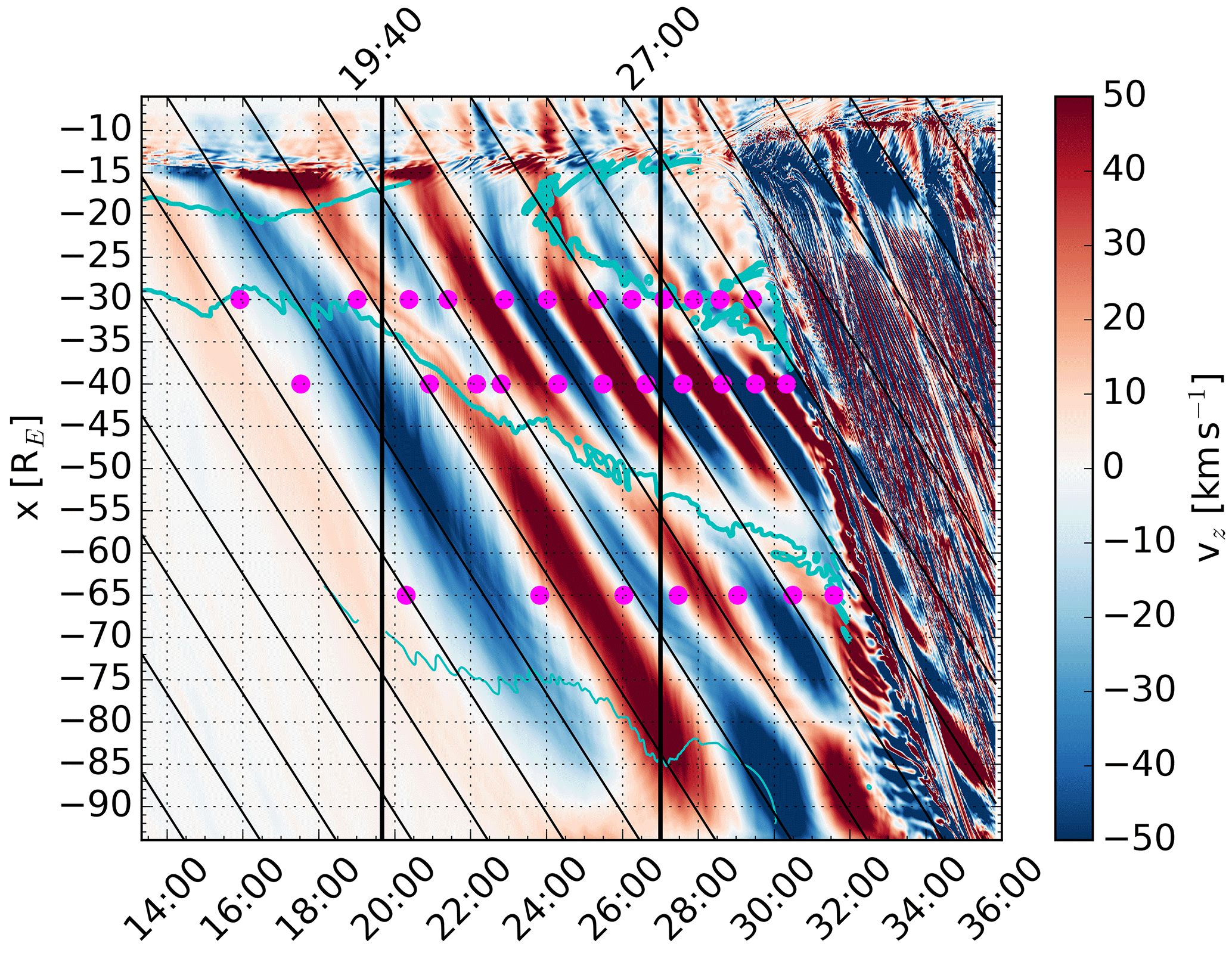
Figure 4The same as Fig. 2 except that the color shows the north component of the ion bulk velocity (Vz). The cyan curves indicate isocontours of pressure in the z direction () with a thicker curve indicating higher pressure: 0.05, 0.1, and 0.2 nPa. The magenta dots mark identified flapping half periods at RE, RE, and RE.
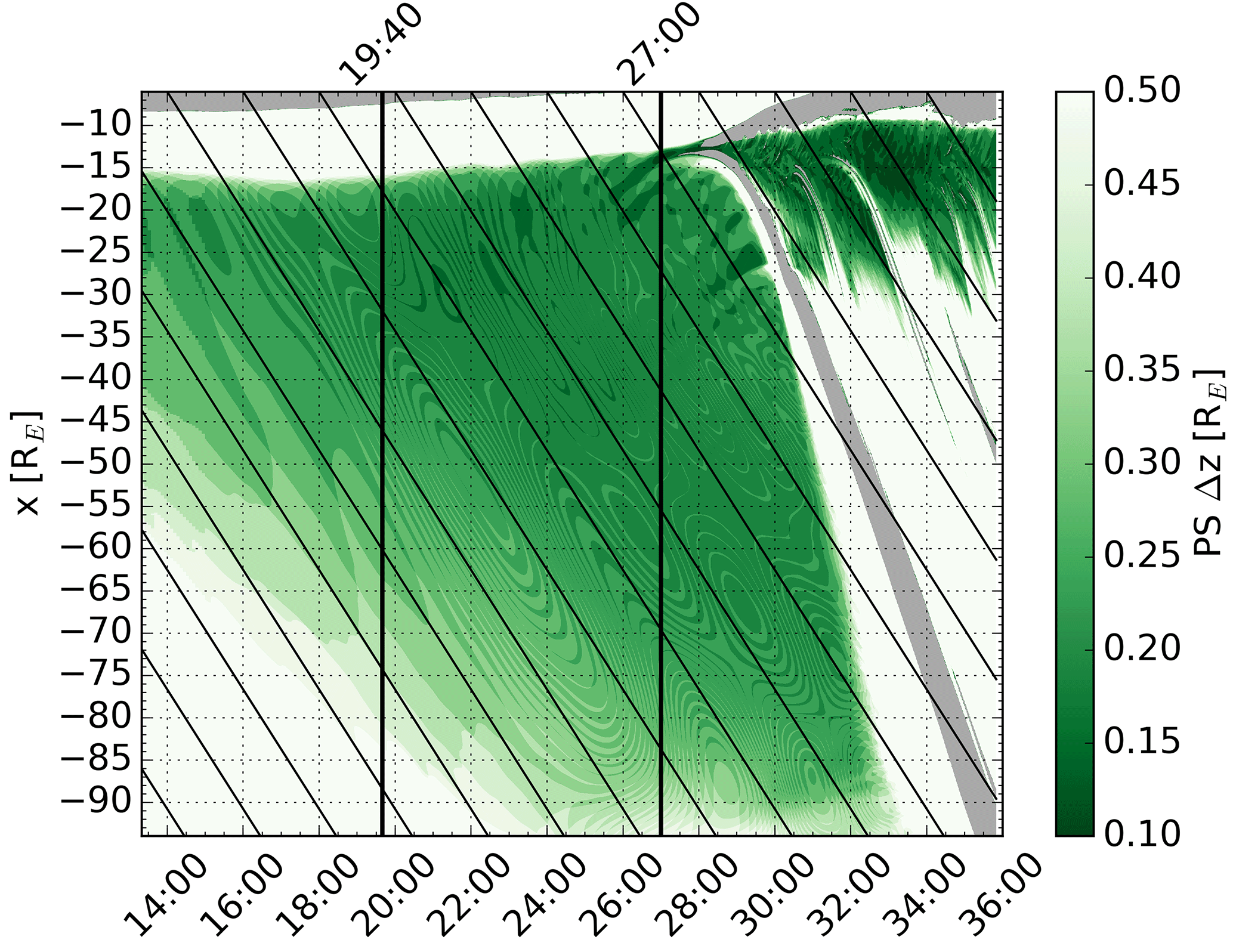
Figures 5 and 6 show the location and thickness of the plasma sheet in the z direction, respectively. The plasma sheet extent in z as a function of x and time was identified as the region between RE where the ion thermal pressure perpendicular to the magnetic field is larger than magnetic pressure () (Wang et al., 2006). The z coordinate was obtained as the mean of the largest and smallest plasma sheet z value, and the thickness as their difference. Gray areas in the plots indicate regions where the condition was not met anywhere between RE. Comparison of Fig. 5 with Fig. 2 shows good correlation between the plasma sheet motion and Bx enhancements, confirming that the enhancements are indeed produced by up and down motion of the plasma sheet. The extent of the motion in the z direction is not very large, less than 1 RE, in agreement with Speiser and Ness (1967), but because the plasma sheet is thin (Fig. 6), this produces significant changes in Bx.

Figure 5The same as Fig. 2 except that the color shows the location of the plasma sheet center in the z direction. Gray areas indicate regions where the location could not be determined.
Finally, before moving on to discuss the drivers of plasma sheet flapping, Fig. 7 shows a time series observed by a virtual satellite located at RE and in the simulation. From top to bottom, the parameters shown are Bx, , Vz, and plasma sheet z location. The vertical magenta lines identify flapping half periods based on sign changes of Vz, and they correspond to the magenta dots at RE in Fig. 4. This plot further clarifies the mutual temporal behavior of the parameters and may be more straightforward to compare with real satellite observations (Sergeev et al., 1998) than the color map plots.
3.2 A driving mechanism for current sheet flapping
At the time shown in Fig. 1, a hemispherically asymmetric magnetopause perturbation, created around the time when subsolar reconnection first started to add new semi-open flux tubes to the lobes, has reached the distance RE (inside the red box). The asymmetric perturbation consists of a simultaneous compression of the northern tail lobe and expansion of the southern tail lobe. The current sheet between the lobes has been shifted slightly southward from its nominal position at z=0. This shift corresponds to the first strong flapping signature (red, starting around RE at ∼16:00) in Fig. 2.
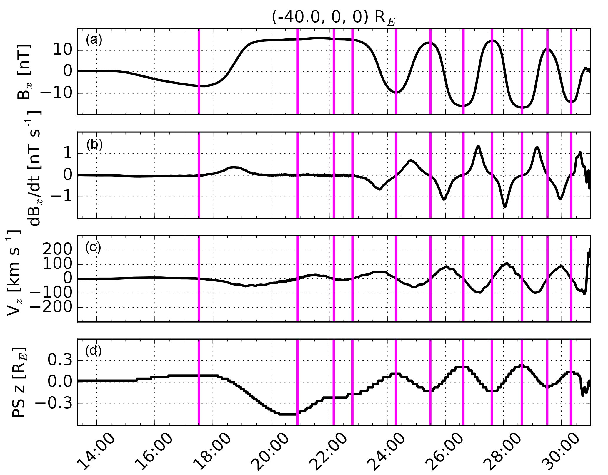
Figure 7Time series observed by a virtual satellite located at RE and in the simulation. From (a) to (d), the parameters shown are earthward component of the magnetic field (Bx, cf. Fig. 2), time derivative of Bx (, cf. Fig. 3), north component of the ion bulk flow (Vz, cf. Fig. 4), and location of the plasma sheet center in the z direction (PS z, cf. Fig. 5). The vertical magenta lines identify flapping half periods based on sign changes of Vz, and they correspond to the magenta dots at RE in Fig. 4.
Figure 8 shows Vz as a function of z and time at y=0 and RE. The vertical black lines are the same as in Fig. 2. The white and magenta (only plotted until 31:00) curves indicate the innermost boundaries where and in the region RE, respectively. The tail lobes are estimated to lie between the white curves (corresponding to the blue curves in Fig. 1).
Figure 8 shows that typically Vz is directed toward the plasma sheet in both lobes, close (roughly within RE) to the plasma sheet where the flapping produces alternating positive and negative values of Vz in both hemispheres (∼24:00–30:00). Close to the magnetopause where localized compressions (e.g., around z=23 RE at 14:00–16:00) and expansions (e.g., around z=23 RE at 16:00–18:00) cause plasma flow toward and away from the plasma sheet, respectively. Furthermore, after 24:00 the magnetopause starts to expand outward due to the accumulation of magnetic flux recently opened by the subsolar reconnection. In these regions, Vz still reflects the motion of the solar wind and is thus directed away from the plasma sheet. The magenta curves in the plot roughly estimate the boundaries between the pre-existing lobe field lines and the newly added lobe field lines.
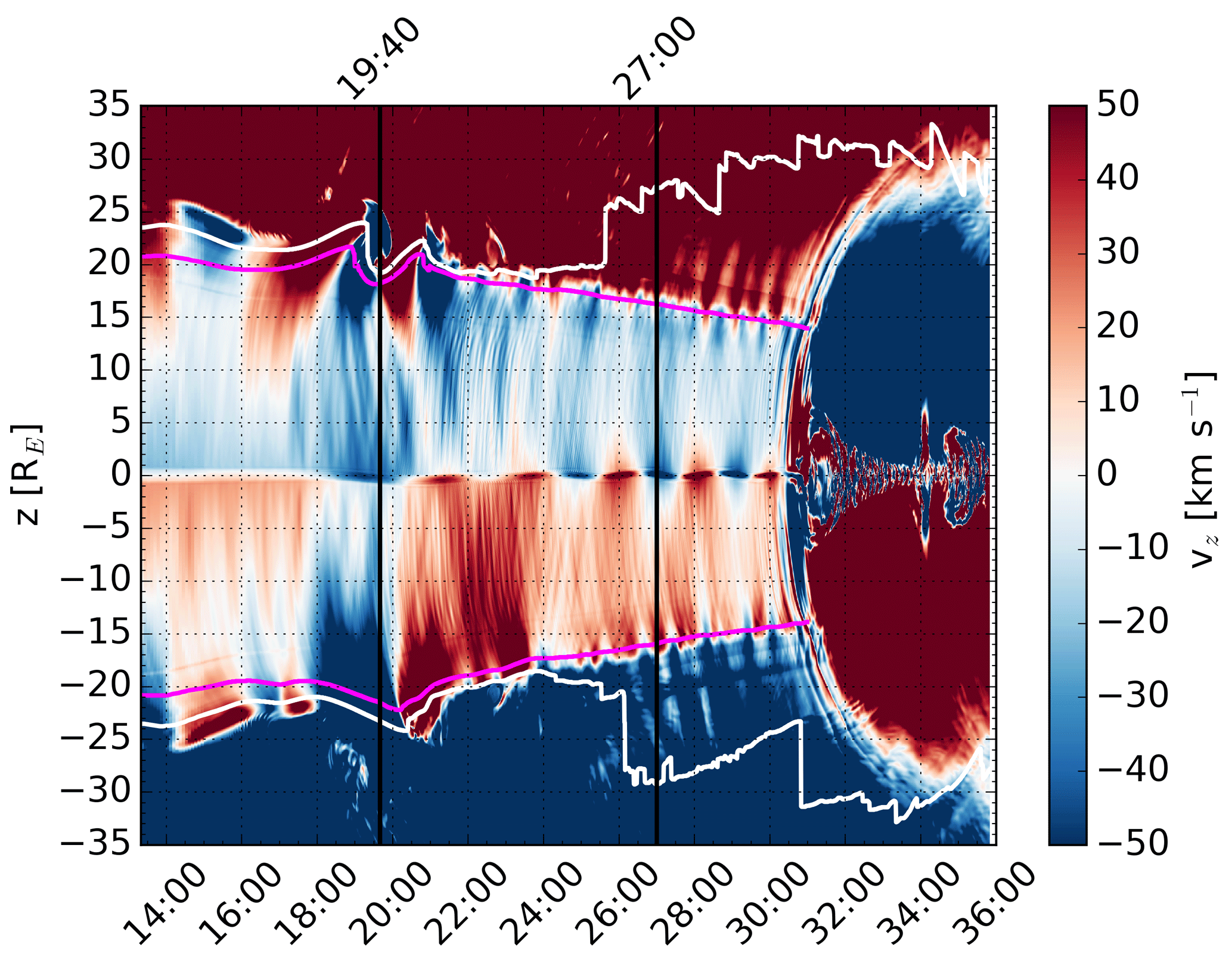
Figure 8North component of the ion bulk velocity (Vz) as a function of z and time at y=0 and RE. The vertical black lines are the same as in Fig. 2. The white and magenta (only plotted until 31:00) curves indicate the innermost boundaries where and in the region RE, respectively. The tail lobes are estimated to lie between the white curves and the magnetosonic wave resonance cavity between the magenta curves.
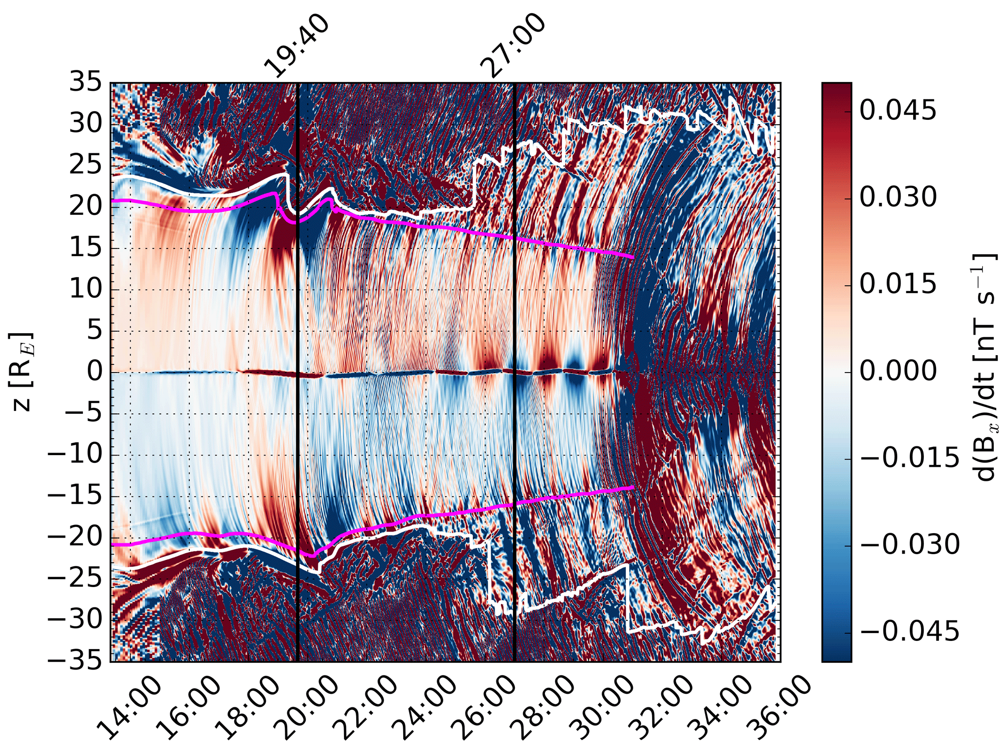
Figure 8 reveals that the passage of the hemispherically asymmetric magnetopause perturbation at the time when the flapping starts around RE is a unique incident. The simultaneous compression of the northern lobe and expansion of the southern lobe causes a downward plasma flow across the entire tail between ∼18:00 and 20:00, which leads to the current sheet shifting downward into the Southern Hemisphere. Only this first flapping signature appears to have a clear magnetopause driver. In order to find out what causes the flapping to continue after the initial driver has passed, Fig. 9 shows the time derivative of Bx in the same format as Fig. 8. At the start of the flapping between 18:00 and 20:00, there is a blue signature in both lobes close to the plasma sheet. This is related to positive Bx in the northern lobe weakening and negative Bx in the southern lobe strengthening. Very close to the plasma sheet the signature is positive as the previously close to zero Bx of the current sheet is replaced by positive Bx as the sheet moves downward. For several minutes (∼20:00–24:00) after this clear initial signature the time derivative of Bx in the lobes consists of small-scale structures, until more coherent, larger-scale signatures associated with strong flapping are established after ∼24:00. The small-scale structure of in the lobes between the initial magnetopause driver and subsequent establishment of the flapping strongly suggests wave activity between the plasma sheet and the magenta curves.
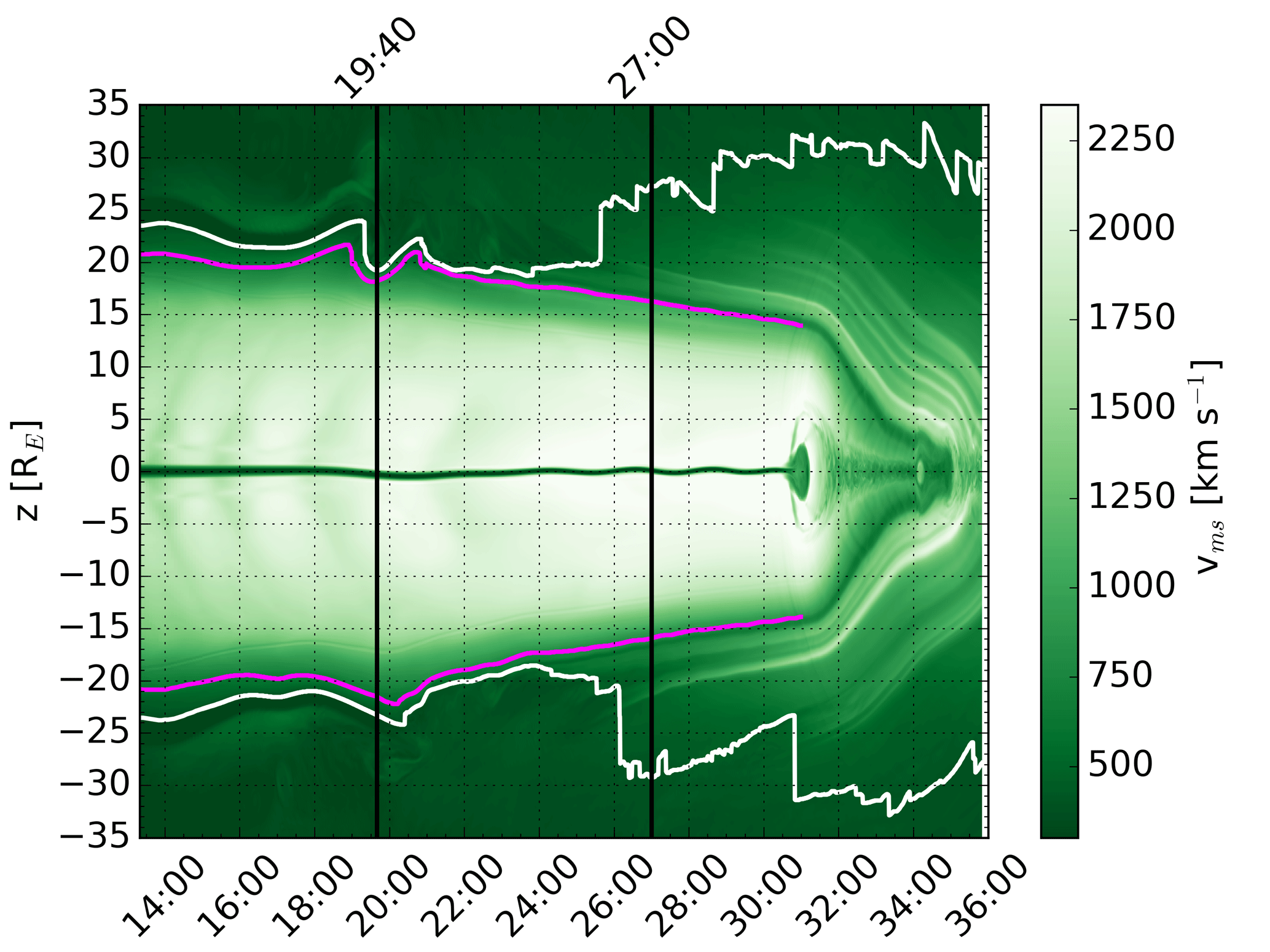
The magnetotail acts both like a waveguide and a resonance cavity (McPherron, 2005). Alfvén waves that tend to propagate down the tail waveguide along the background lobe magnetic field lines are eventually lost. Magnetosonic waves that propagate perpendicular to the background magnetic field can form standing waves in the tail resonance cavity at a roughly constant distance from the Earth. A tailward propagating displacement of the boundary of the cavity produces a disturbance inside the magnetosphere that stands in the x−z direction while propagating down the tail. Figure 10 shows the magnetosonic speed (Vms) across the tail at the distance RE. There is a distinct change in the magnetosonic speed near the location of the magenta curves. This would explain why the waves in Fig. 9 appear to reflect there. We estimate that the magnetosonic wave resonance cavity lies between these curves.
Standing waves are only possible at discrete frequencies. The simplest approximation to the fundamental period can be obtained by integrating the magnetosonic travel time across the cavity (or back and forth across one hemisphere of the cavity). Figure 11 shows the travel time across half of the magnetotail resonance cavity (T∕2) at distances RE (black), RE (red), and RE (blue) as a function of time (solid curves). For example, T∕2 at RE has been estimated by integrating over the distance between the magenta curves marked in Fig. 10 and dividing by 2. The dots in Fig. 11 indicate tail flapping half periods with color indicating the corresponding x coordinate. The flapping half periods have been obtained as the time differences between consecutive magenta dots indicated in Fig. 4, and they have been associated with a time stamp corresponding to the average of the two times. The dashed vertical lines mark the start and end times of the first flapping signature at the three distances.
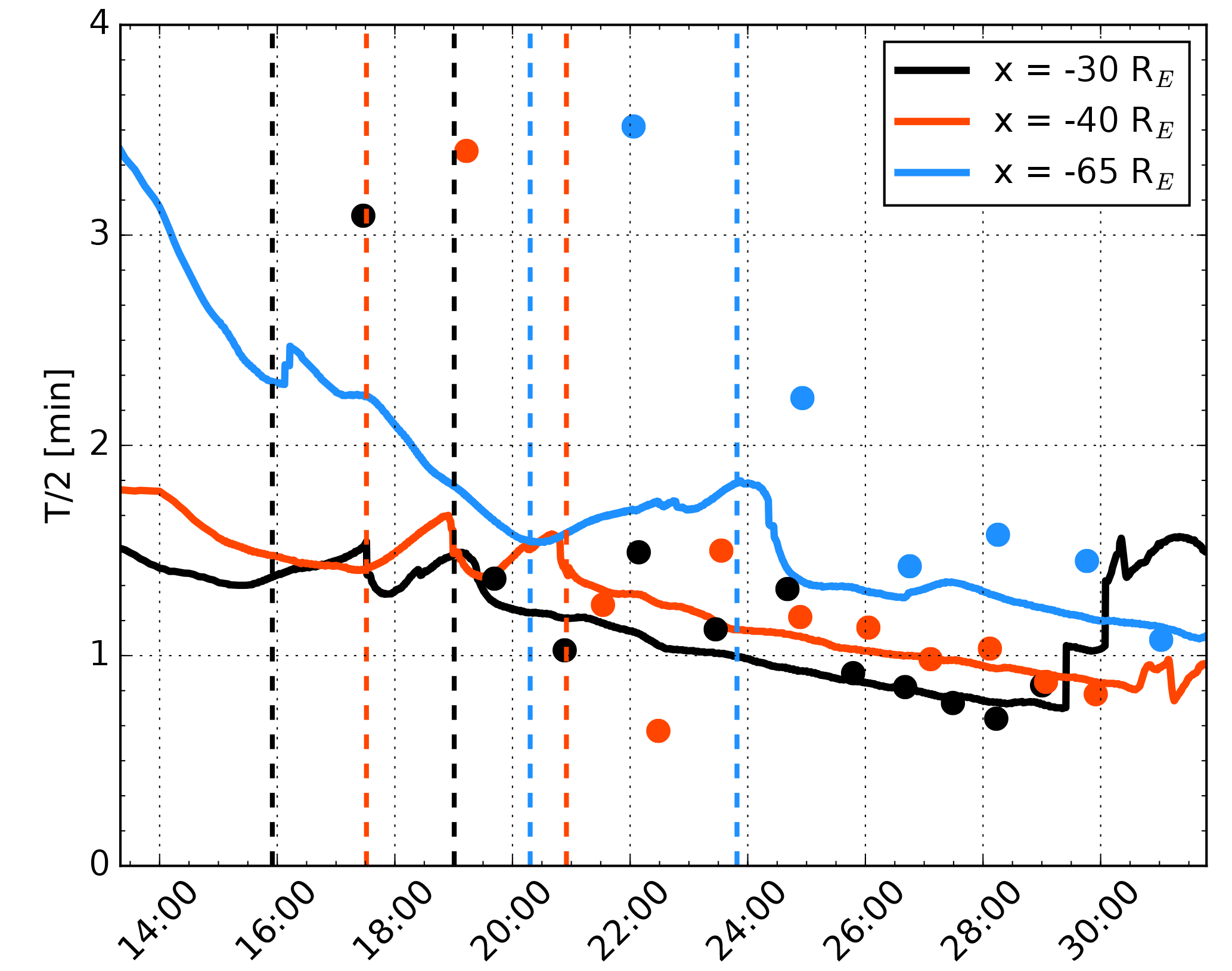
Figure 11Travel time of magnetosonic waves across half of the magnetotail resonance cavity (T∕2) at distances RE (black), RE (red), and RE (blue) as a function of time (solid curves). For example, T∕2 at RE has been estimated by integrating over the distance between the magenta curves marked in Fig. 10 and dividing by 2. The dots indicate tail flapping half periods with color indicating the corresponding x coordinate. The flapping half periods have been obtained as the time differences between consecutive magenta dots indicated in Fig. 4, and they have been associated with a time stamp corresponding to the average of the two times. The dashed vertical lines show the start and end times of the first flapping signature at the three distances.
The travel time at a given distance decreases with increasing time as the increase in pressure due to the addition of flux tubes opened by subsolar reconnection compresses the lobes, decreasing the cross section of the cavity and increasing the magnetosonic speed within. The bumps in the travel time during the first flapping signature at all three x distances are associated with the magnetopause perturbation that initiated the flapping. Apart from the first flapping signature at a given distance, there appears to be a good correspondence between the approximated local magnetosonic travel time across half of the resonance cavity and the observed flapping half period. Both Figs. 11 and 4 show that the period of the flapping signatures increases with increasing distance away from the Earth. At a given location, the period decreases with increasing time. These changes follow the structure and development of pressure indicated in Fig. 4 by the cyan curves. Higher pressure indicates a smaller cross section of the cavity and higher magnetosonic speed due to the higher magnetic field strength, which is in agreement with the suggestion that the local flapping period is determined by the bounce time of the magnetosonic waves within the cavity.
We have examined current sheet flapping in Vlasiator and suggested a source mechanism that is capable of initiating and maintaining flapping in the central meridian of the magnetotail before and during tail reconnection when the plasma sheet is thin. According to our suggested mechanism, the flapping is initiated by a hemispherically asymmetric perturbation of the magnetopause that is capable of displacing the current sheet from its nominal position. The perturbation travels tailward along the magnetopause (close to the solar wind speed in this case), producing a current sheet displacement that propagates tailward at the same speed. As the first flapping signature is directly driven by the magnetopause perturbation, no correspondence between the duration of flapping signature and the local magnetosonic wave travel time in Fig. 11 is expected. The initial current sheet displacement launches a standing magnetosonic wave within the local resonance cavity. The travel time of the wave within the cavity determines the period of the subsequent flapping signatures, as shown in Fig. 11. Changes in the cross-sectional width of the cavity as well as the magnetosonic speed within the cavity affect the wave travel time and thus the local flapping period. The flapping signatures that can be produced by our suggested mechanism are compliant with the characteristics of plasma sheet flapping in the center of the tail cited in the Introduction.
We do not observe a damping of the current sheet flapping. On the contrary, after the initial displacement, the signature can even strengthen (e.g., at RE in 24:00–28:00 in Fig. 2). The reason for this could be the continued compression of the cavity that could provide additional energy to the standing wave.
In our polar plane simulation driven by steady solar wind, the initiating magnetopause perturbation is created by subsolar reconnection. In 3-D, such a perturbation could have a finite extent in the y direction, and propagate tailward along the noon–midnight sector magnetopause. Thus, the created plasma sheet flapping in the midnight sector plasma sheet could act as a source of the dawnward and duskward propagating flapping signatures that have been observed by satellites (Sergeev et al., 2004). A solar wind perturbation, such as a tilted interplanetary shock, might also be able to produce the initial plasma sheet displacement, but probably not in such a localized manner (in y), as solar wind structures tend to be of much larger-scale sizes. Any hemispherically asymmetric magnetopause perturbation could cause tail flapping as presented here, but the shown perturbation initiated by subsolar magnetopause reconnection is a good example of a perturbation confirmed by simulation which indeed does cause this. However, the perturbation initiating the flapping need not necessarily be at the magnetopause. Any disturbance capable of displacing the current sheet, a BBF for example, should be able to initiate the flapping.
For the purposes of further validation against satellite observations, our model predicts that, e.g., the flapping period at a given observation location should decrease with increasing pressure in the lobes.
We have used a polar plane simulation from the global hybrid-Vlasov model Vlasiator, driven by steady southward IMF and fast solar wind, to study the characteristics and source of current sheet flapping signatures in the magnetotail. Because the simulation is 2-D, we concentrated on the flapping in the center of the tail. Our main results are as follows.
-
The characteristics of the simulated flapping signatures agree with observations reported in the literature.
-
In the simulation, the flapping is initiated by a hemispherically asymmetric magnetopause perturbation, created by subsolar reconnection, that is capable of displacing the tail current sheet from its nominal position. The current sheet displacement propagates downtail together with the driving magnetopause perturbation.
-
As the initial current sheet displacement passes, it launches a standing magnetosonic wave within the local tail resonance cavity. The travel time of the wave within the cavity determines the period of the subsequent flapping signatures.
-
Increasing pressure in the tail lobes due to an increasing amount of open magnetic flux added by subsolar reconnection can affect the cross-sectional width of the resonance cavity as well as the magnetosonic speed within the cavity. These in turn affect the wave travel time and flapping period. The compression of the resonance cavity may also provide additional energy to the standing wave, which may lead to strengthening of the flapping signature.
The suggested mechanism could act as a source of kink-like waves that are emitted from the center of the tail and propagate toward the dawn and dusk flanks. However, further research using a 3-D simulation will be needed to examine this suggestion.
Vlasiator is an open source code released under the GPLv2 license. The code is available at http://github.com/fmihpc/vlasiator (last access: 25 July 2018, Palmroth and the Vlasiator team, 2018).
LJ carried out most of the analysis and prepared the manuscript. YPK participated in running the simulation and development of the analysis methods. UG participated in development of the analysis methods. All co-authors actively participated in the analysis and discussion of the results.
The authors declare that they have no conflict of interest.
We acknowledge The European Research Council for Starting grant
200141-QuESpace, with which Vlasiator
(http://www.physics.helsinki.fi/vlasiator, last access: 25 July 2018)
was developed, and Consolidator grant 682068-PRESTISSIMO awarded for further
development of Vlasiator and its use in scientific investigations. We
gratefully acknowledge Academy of Finland grant numbers 267144 and 309937.
The work leading to these results has been partially carried out in the
Finnish Centre of Excellence in Research of Sustainable Space (Academy of
Finland grant number 312351). PRACE (http://www.prace-ri.eu, last
access: 25 July 2018) is acknowledged for granting us Tier-0 computing time
in HLRS Stuttgart, where Vlasiator was run in the HazelHen machine with
project number 2014112573. The work of LT is supported by a
Marie Sklodowska-Curie Individual Fellowship (no. 704681).
The topical editor, Anna Milillo, thanks two anonymous
referees for help in evaluating this paper.
Daldorff, L. K. S., Tóth, G., Gombosi, T. I., Lapenta, G., Amaya, J., Markidis, S., and Brackbill, J. U.: Two-way coupling of a global Hall magnetohydrodynamics model with a local implicit particle-in-cell model, J. Comput. Phys., 268, 236–254, https://doi.org/10.1016/j.jcp.2014.03.009, 2014. a
Davey, E. A., Lester, M., Milan, S. E., and Fear, R. C.: Storm and substorm effects on magnetotail current sheet motion, J. Geophys. Res., 117, A02202, https://doi.org/10.1029/2011JA017112, 2012. a
Erkaev, N. V., Semenov, V. S., Kubyshkin, I. V., Kubyshkina, M. V., and Biernat, H. K.: MHD model of the flapping motions in the magnetotail current sheet, J. Geophys. Res., 114, A03206, https://doi.org/10.1029/2008JA013728, 2009. a
Forsyth, C., Lester, M., Fear, R. C., Lucek, E., Dandouras, I., Fazakerley, A. N., Singer, H., and Yeoman, T. K.: Solar wind and substorm excitation of the wavy current sheet, Ann. Geophys., 27, 2457–2474, https://doi.org/10.5194/angeo-27-2457-2009, 2009. a
Gabrielse, C., Angelopoulos, V., Runov, A., Kepko, L., Glassmeier, K. H., Auster, H. U., McFadden, J., Carlson, C. W., and Larson, D.: Propagation characteristics of plasma sheet oscillations during a small storm, Geophys. Res. Lett., 35, L17S13, https://doi.org/10.1029/2008GL033664, 2008. a
Golovchanskaya, I. V. and Maltsev, Y. P.: On the identification of plasma sheet flapping waves observed by Cluster, Geophys. Res. Lett., 32, L02102, https://doi.org/10.1029/2004GL021552, 2005. a
Hoilijoki, S., Ganse, U., Pfau-Kempf, Y., Cassak, P. A., Walsh, B. M., Hietala, H., von Alfthan, S., and Palmroth, M.: Reconnection rates and X line motion at the magnetopause: Global 2D-3V hybrid-Vlasov simulation results, J. Geophys. Res.-Space, 122, 2877–2888, https://doi.org/10.1002/2016JA023709, 2017. a
Jarvinen, R., Vainio, R., Palmroth, M., Juusola, L., Hoilijoki, S., Pfau-Kempf, Y., Ganse, U., Turc, L., and von Alfthan, S.: Ion acceleration by flux transfer events in the terrestrial magnetosheath, Geophys. Res. Lett., 45, 1723–1731, https://doi.org/10.1002/2017GL076192, 2018. a
Laitinen, T. V., Nakamura, R., Runov, A., Rème, H., and Lucek, E. A.: Global and local disturbances in the magnetotail during reconnection, Ann. Geophys., 25, 1025–1035, https://doi.org/10.5194/angeo-25-1025-2007, 2007. a, b
McPherron, R. L.: Magnetic Pulsations: Their Sources and Relationto Solar Wind and Geomagnetic Activity, Surv. Geophys., 26, 545–592, https://doi.org/10.1007/s10712-005-1758-7, 2005. a
Palmroth, M. and the Vlasiator team: Vlasiator: hybrid-Vlasov simulation code, Github repository, available at: https://github.com/fmihpc/vlasiator/ (last access: 25 July 2018), 2018. a
Palmroth, M., Honkonen, I., Sandroos, A., Kempf, Y., von Alfthan, S., and Pokhotelov, D.: Preliminary testing of global hybrid-Vlasov simulation: Magnetosheath and cusps under northward interplanetary magnetic field, J. Atmos. Sol.-Terr. Phy., 99, 41–46, https://doi.org/10.1016/j.jastp.2012.09.013, 2013. a
Palmroth, M., Archer, M., Vainio, R., Hietala, H., Pfau-Kempf, Y., Hoilijoki, S., Hannuksela, O., Ganse, U., Sandroos, A., von Alfthan, S., and Eastwood, J. P.: ULF foreshock under radial IMF: THEMIS observations and global kinetic simulation Vlasiator results compared, J. Geophys. Res.-Space, 120, 8782–8798, https://doi.org/10.1002/2015JA021526, 2015. a
Palmroth, M., Hoilijoki, S., Juusola, L., Pulkkinen, T. I., Hietala, H., Pfau-Kempf, Y., Ganse, U., von Alfthan, S., Vainio, R., and Hesse, M.: Tail reconnection in the global magnetospheric context: Vlasiator first results, Ann. Geophys., 35, 1269–1274, https://doi.org/10.5194/angeo-35-1269-2017, 2017. a, b, c
Petrukovich, A. A., Baumjohann, W., Nakamura, R., and Runov, A.: Formation of current density profile in tilted current sheets, Ann. Geophys., 26, 3669–3676, https://doi.org/10.5194/angeo-26-3669-2008, 2008. a
Rong, Z. J., Shen, C., Petrukovich, A. A., Wan, W. X., and Liu, Z. X.: The analytic properties of the flapping current sheets in the earth magnetotail, Planet. Space Sci., 58, 1215–1229, https://doi.org/10.1016/j.pss.2010.04.016, 2010. a
Rong, Z. J., Barabash, S., Stenberg, G., Futaana, Y., Zhang, T. L., Wan, W. X., Wei, Y., and Wang, X.-D.: Technique for diagnosing the flapping motion of magnetotail current sheets based on single-point magnetic field analysis, J. Geophys. Res.-Space, 120, 3462–3474, https://doi.org/10.1002/2014JA020973, 2015. a, b
Runov, A., Nakamura, R., Baumjohann, W., Zhang, T. L., Volwerk, M., Eichelberger, H.-U., and Balogh, A.: Cluster observation of a bifurcated current sheet, Geophys. Res. Lett., 30, 1036, https://doi.org/10.1029/2002GL016136, 2003. a
Runov, A., Angelopoulos, V., Sergeev, V. A., Glassmeier, K.-H., Auster, U., McFadden, J., Larson, D., and Mann, I.: Global properties of magnetotail current sheet flapping: THEMIS perspectives, Ann. Geophys., 27, 319–328, https://doi.org/10.5194/angeo-27-319-2009, 2009. a, b
Sergeev, V., Angelopoulos, V., Carlson, C., and Sutcliffe, P.: Current sheet measurements within a flapping plasma sheet, J. Geophys. Res., 103, 9177–9187, https://doi.org/10.1029/97JA02093, 1998. a, b, c, d, e, f, g, h, i
Sergeev, V., Runov, A., Baumjohann, W., Nakamura, R., Zhang, T. L., Volwerk, M., Balogh, A., Rème, H., Sauvaud, J. A., André, M., and Klecker, B.: Current sheet flapping motion and structure observed by Cluster, Geophys. Res. Lett., 30, 1327, https://doi.org/10.1029/2002GL016500, 2003. a
Sergeev, V., Runov, A., Baumjohann, W., Nakamura, R., Zhang, T. L., Balogh, A., Louarn, P., Sauvaud, J.-A., and Réme, H.: Orientation and propagation of current sheet oscillations, Geophys. Res. Lett., 31, L05807, https://doi.org/10.1029/2003GL019346, 2004. a, b, c
Sergeev, V. A., Sormakov, D. A., Apatenkov, S. V., Baumjohann, W., Nakamura, R., Runov, A. V., Mukai, T., and Nagai, T.: Survey of large-amplitude flapping motions in the midtail current sheet, Ann. Geophys., 24, 2015–2024, https://doi.org/10.5194/angeo-24-2015-2006, 2006. a
Sergeev, V. A., Tsyganenko, N. A., and Angelopoulos, V.: Dynamical response of the magnetotail to changes of the solar wind direction: an MHD modeling perspective, Ann. Geophys., 26, 2395–2402, https://doi.org/10.5194/angeo-26-2395-2008, 2008. a
Shen, C., Rong, Z. J., Li, X., Dunlop, M., Liu, Z. X., Malova, H. V., Lucek, E., and Carr, C.: Magnetic configurations of the tilted current sheets in magnetotail, Ann. Geophys., 26, 3525–3543, https://doi.org/10.5194/angeo-26-3525-2008, 2008. a
Speiser, T. W. and Ness, N. F.: The neutral sheet in the geomagnetic tail: Its motion, equivalent currents, and field line connection through it, J. Geophys. Res., 72, 131–141, https://doi.org/10.1029/JZ072i001p00131, 1967. a, b, c
Sun, W.-J., Fu, S., Shi, Q., Zong, Q.-G., Yao, Z., Xiao, T., and Parks, G.: THEMIS observation of a magnetotail current sheet flapping wave, Chinese Sci. Bull., 59, 154–161, 2013. a
von Alfthan, S., Pokhotelov, D., Kempf, Y., Hoilijoki, S., Honkonen, I., Sandroos, A., and Palmroth, M.: Vlasiator: First global hybrid-Vlasov simulations of Earth's foreshock and magnetosheath, J. Atmos. Sol.-Terr. Phy., 120, 24–35, https://doi.org/10.1016/j.jastp.2014.08.012, 2014. a
Wang, C., Lyons, L. R., Weygand, J. M., Nagai, T., and McEntire, R. W.: Equatorial distributions of the plasma sheet ions, their electric and magnetic drifts, and magnetic fields under different interplanetary magnetic field Bz conditions, J. Geophys. Res., 111, A04215, https://doi.org/10.1029/2005JA011545, 2006. a
Wei, X. H., Cai, C. L., Cao, J. B., Rème, H., Dandouras, I., and Parks, G. K.: Flapping motions of the magnetotail current sheet excited by nonadiabatic ions, Geophys. Res. Lett., 42, 4731–4735, https://doi.org/10.1002/2015GL064459, 2015. a
Zelenyi, L. M., Artemyev, A. V., Petrukovich, A. A., Nakamura, R., Malova, H. V., and Popov, V. Y.: Low frequency eigenmodes of thin anisotropic current sheets and Cluster observations, Ann. Geophys., 27, 861–868, https://doi.org/10.5194/angeo-27-861-2009, 2009. a
http://www.physics.helsinki.fi/vlasiator,
last access: 25 July 2018