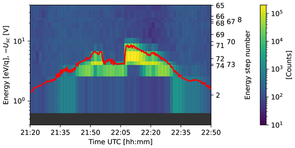
Flying through the plasmasphere to optimize low-energy ion measurements

The Juice flyby of Earth in August 2024 gave us the first chance to evaluate the performance of the Jovian Plasma Dynamics and Composition analyzer (JDC) in environments similar to those expected at Jupiter. JDC is one of the sensors belonging to the Particle Environment Package (PEP) on the Juice spacecraft. It measures positive and negative ions as well as electrons in the energy range 1 eV q⁻¹ to 35 keV q⁻¹. One of the most challenging observations at the final destination is the one of the low-energy ion populations in the tenuous ionospheres of Jupiter's icy moons. During the Juice flyby of Earth we discovered that the energies of the positive ions observed by JDC were not easy to interpret due to a problem with the energy sweep. Using measurements made on ground, we were able to reconstruct the observed energies and construct a new sweeping scheme that solves the problem and that will greatly improve future observations. We also used a simulation to explain the effects of the spacecraft velocity and spacecraft potential on the recorded positive ion fluxes when Juice passed through the Earth's plasmasphere. The study highlights the importance of in-flight calibrations for optimizing the scientific return. Planetary flybys give access to multiple low-energy particle populations besides the mono-energetic and highly directional solar wind.

1 Introduction

As one of the three large icy moons around Jupiter, Ganymede is a main target for the Jupiter Icy Moons Explorer (Juice) mission (Grasset et al., 2013). The largest moon in the solar system is also the only one to have an intrinsic magnetic field (Kivelson et al., 1996), which, together with the complex interaction with Jupiter, gives rise to auroral emissions on the moon. These emissions have been observed from Earth orbit with the Hubble Space Telescope (Hall et al., 1998; McGrath et al., 2013) and the presence of molecular oxygen as a major constituent of Ganymede's thin atmosphere has been inferred (Vorburger et al., 2024). The atmosphere results from sublimation, radiolysis and sputtering (Hansen et al., 2022) of the icy surface, which consists of water ice and non-ice components that can host volatiles (Tosi et al., 2024). Parts of the neutral atmosphere is ionized by photoionization and electron impact ionization (Masters et al., 2025). The ionosphere has been directly detected in situ during Galileo (Frank et al., 1997) and Juno (Valek et al., 2022) flybys, as well as through radio occultation measurements (e.g., Buccino et al., 2022). Frank et al. (1997) reported a dense and cold plasma close to Ganymede. They suggested that the ions moving away from the moon were H⁺, but this has later been questioned (Vasyliūnas and Eviatar, 2000). The Juno flyby observed both atomic and molecular oxygen and hydrogen ions (Valek et al., 2022). They also detected H${}_{\mathrm{3}}^{+}$, which suggests that the exosphere is not collisionless. H${}_{\mathrm{3}}^{+}$ does not form through ionization but is the result of chemistry. The presence of H${}_{\mathrm{3}}^{+}$ implies an ion-neutral chemistry, which may lead to a more complex composition (Beth et al., 2025).

Both the initial acceleration (to the first few eV) of cold ionospheric plasma and ion-neutral coupling are fundamental astrophysical problems with applications throughout the solar system and beyond. Atmospheric escape has been observed from Earth (André and Yau, 1997) and many other solar system bodies (e.g., Brain et al., 2016) as well as from exoplanets (Owen, 2019). Yet, the process responsible for the initial energization of the escaping plasma is not well-known (e.g., Hanley et al., 2022). Knowledge about the coupling to the neutral gas is an integral part in the understanding of the evolution of low-energy ion populations (Vorburger et al., 2024). The energy budget of the Ganymede ionosphere, the role of collisions and transport of the ionospheric plasma are all key topics for the Juice mission (Masters et al., 2025).

The Jovian Plasma Dynamics and Composition Analyzer (JDC; Wittmann, 2022), part to the Particle Environment Package (PEP; Galli et al., 2022), is one of the sensors on Juice designed to observe the low-energy ion populations at Jupiter's icy moons. Such observations are not trivial. Due to the interaction between the spacecraft and its environment a spacecraft gets electrically charged. Whether the spacecraft potential is negative or positive depends on the plasma environment, and is decided by a current balance (Garrett, 1981; Whipple, 1981). The main contributing currents are often the photoelectron current and the electron current. The photoelectron current is the result of solar photons causing emission of electrons from the spacecraft surface, driving the spacecraft positive. The electron current is carried by the electrons in the plasma colliding with the spacecraft, driving it negative. As the plasma electrons are more mobile than the ions, the ion current is often negligible. In a dense plasma the electron current dominates over the photoelectron current charging the spacecraft negative. This happens for spacecraft in the Earth’s plasmasphere (e.g., Kim et al., 2022; Zeroual et al., 2026) and Juice is expected to charge negatively in the ionospheres of Europa and Ganymede (Bochet et al., 2023). A charged spacecraft prevents low-energy ions with the same charge from reaching the detectors. As an example, near-Earth space has been visited by a multitude of spacecraft but the outflow of cold H⁺ ions still went undiscovered due positively charged spacecraft. It was finally observed with the Cluster spacecraft using indirect methods (Sauvaud et al., 2001; Engwall et al., 2006; André, 2015). The Rosetta spacecraft, which accompanied comet 67P/Churyumov-Gerasimenko for two years, charged up to a surprisingly high negative potential. This enabled the detection of the cold population of H₂O⁺ flowing radially away from the comet nucleus (Stenberg Wieser et al., 2017; Bergman et al., 2020, 2021). In general, low-energy ions become observable by particle detectors only when there is a significant relative velocity between the ion population and the spacecraft (ram-effect) or when the spacecraft is charged, such that the ions are accelerated towards the instrument. In both cases, the original ion velocity distribution functions get distorted, and the measurements must be corrected to remove the effect of the spacecraft. The distortion of the ion trajectories also mean that field-of-view obstruction by structures on the spacecraft is energy-dependent and hard to predict (Barrie et al., 2019; Bochet et al., 2023).

Another challenge with low-energy ion observations is that the energy coverage of an instrument at low energies often is sparse. This is a consequence of the use of an electrostatic analyzer for energy selection. The passband width of an electrostatic analyzer is proportional to its centre energy. This means that for energies below 10–20 eV many energy steps would be needed to densely cover a range of a few eV. At the same time the number of energy steps that can be used is limited for timing and telemetry reasons. A common approach is to use linear energy stepping below a certain energy and logarithmic stepping above.

It is often impossible to make a calibration on ground of the instrument at the lowest energies. The calibration system where JDC was calibrated has difficulties to produce suitably intense ion beams with energies of only a few eV (Wuest et al., 2007). Dedicated low-energy sources exist (Rubin et al., 2006), but were not used for JDC for schedule reasons. Hence, the response of JDC to ion energies of a few eV was only extrapolated from higher energy measurements, and not explicitly measured. The possibility to make measurements in a space environment prior to the start of the Juice science phase is therefore extremely valuable.

During Juice flyby of Earth on 20 August 2024, the spacecraft passed through the Earth's plasmasphere. This region with cold plasma is similar to, for example, the ionosphere of Ganymede and the observations made by JDC enabled judging the sensor's ability to perform low-energy ion measurements. The problems we discovered were understood and solved with the help of laboratory measurements and simulations. This paper describes how JDC's capabilities to make low-energy ion observations at the final destination were optimized through a combination of space observations and measurements on ground.

2 Instrumentation

The Jovian Plasma Dynamics and Composition Analyzer (JDC; Wittmann, 2022) is one of six sensors constituting the Particle Environment Package (PEP) on Juice. PEP measures neutral as well as electrically charged particles over a large energy range (<0.001 eV to >1 MeV) (Galli et al., 2022). JDC covers the mid-energy regime (1 eV q⁻¹–35 keV q⁻¹) and is capable of measuring both positively and negatively charged ions as well as electrons. Its field-of-view is one hemisphere (2π sr) but together with the complementary sensor JEI (Jovian Electron and Ion Analyzer), placed on the opposite side of the spacecraft, coverage of $\mathrm{7}/\mathrm{8}$ of the full sky is achieved. The mass resolution of JDC is enough to distinguish the major ions in the Jovian system, such as hydrogen and various charge states of sulphur and oxygen ($m/\mathrm{\Delta }m>\mathrm{20}$).

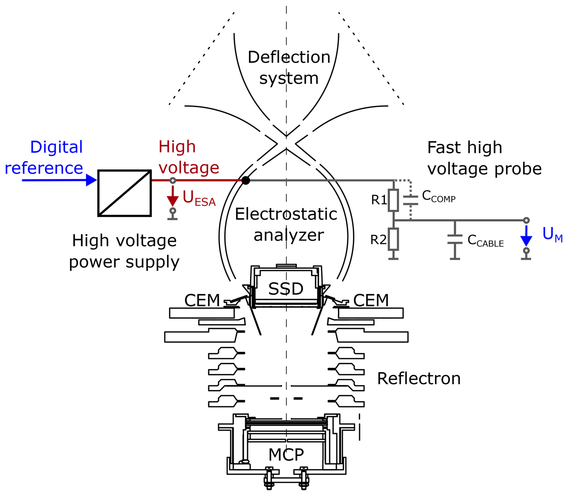
Figure 1 JDC cross section, showing the deflection system, the electrostatic analyzer and the reflectron with the time-of-flight start channel electron multipliers (CEMs), time-of-flight stop micro channel plate (MCP) and the anti-coincidence solid state detector (SSD). The high voltage on the electrostatic analyzer (U_ESA) is measured on ground using a fast high voltage probe resulting in a voltage U_M proportional to voltage U_ESA.

Figure 1 shows a cross section of the ion optical system of JDC. The sensor determines the direction of arrival of an observed particle. The arrival directions perpendicular to instrument symmetry axis are divided into 16 azimuth sectors that are registered simultaneously. Arrival directions in an angular range of ϕ=0–90° with respect to the symmetry axis are covered with an elevation angle sweep. Different electric potential settings on the deflector electrodes allow particles arriving from different (elevation) angles to pass through the deflection system.

A particle passing through the deflection system enters the electrostatic analyzer (ESA). The ESA consists of two curved plates over which a voltage is applied to allow only particles with a specific energy to pass between them. The ESA in JDC is a modified classical top-hat spherical analyzer (Carlson et al., 1982; Kazama, 2013). The inner electrode is not spherical but sectorized, that is, composed of 16 wedges (Stude, 2016). The outer electrode has an ellipsoid cross-section (Stude, 2016). The result is a variable gap width between the two electrodes and hence a slightly stronger electric field at the edges of the wedges compared to the centre. This results in an almost rectangular shape of the response of a sector in azimuthal direction. The design reduces the diameter of the ESA with 30 % and maintains sufficient transmittance and energy resolution without increasing the maximum analyzer voltage. The energy resolution is $\mathrm{\Delta }E/E=\mathrm{15}\mathit{\%}$. For each of the 12 elevations steps, JDC sweeps through 75 energies. Each energy sweep takes 960 ms and the total measurement cycle including extra waiting times is made in 11.69 s.

To separate between different masses per charge JDC uses the time-of-flight approach with a linear electric field reflectron (Gilbert et al., 2010; McComas et al., 1990). In the cylindrical volume of the reflectron, an electric field is created that increases linearly along the symmetry axis. Particles enter the reflectron section through a start surface assembly. As a particle scatters at the start surface it creates one or more secondary electrons, which are registered by one of the 16 start channel electron multipliers (CEMs), each corresponding to one azimuthal direction of arrival (perpendicular to the symmetry axis of the instrument). The flight time is measured between the start signal and the corresponding signal from the stop micro channel plate (MCP). Optionally, for particles reflected in the reflectron, the stop signal can be vetoed by a solid state detector (SSD). Species with same mass per charge, e.g., O⁺ and S²⁺, can only be statistically separated using the different energy loss at the time-of-flight start surface. By changing the polarity of the voltages applied to the electrostatic analyser and the deflection system electrodes, JDC can alternatively measure positively charged ions or negatively charged ions and electrons.

In addition to data from JDC, we use an estimate of the spacecraft potential obtained from the Radio & Plasma Wave Investigation (RPWI; Wahlund et al., 2025). The spacecraft potential is directly measured by the P4 Langmuir probe in single ended mode and is accurate to within 10 %.

3 Observations in space

During the Lunar-Earth Gravity assist (LEGA) on 19–20 August 2024, JDC was turned on and generated science data. Figure 2 shows the orbit geometry, where the spacecraft approaches Earth along the magnetotail, performs the Moon gravity assist (cross in the far tail) and continues towards Earth. In this paper we concentrate on the positive ion data recorded within 1.5 h around the Earth closest approach. The relevant period is marked with a thick black line along the orbit trajectory in Fig. 2.

Figure 2 The trajectory of Juice during LEGA in geocentric solar ecliptic (GSE) coordinates (black line). Juice moves from left to right in the figure. The time period from 21:20 to 22:50 UTC on 20 August 2024 is indicated with a wide black line along the trajectory. The Moon is indicated by the X-symbol and the Earth is represented by a circle. The red circular disk schematically shows the plasmasphere. A model bow shock (solid blue line; Chao et al., 2002) is shown along with a model magnetopause (dashed blue line; Shue et al., 1997).

The Earth flyby brought Juice within two Earth radii from the centre of the planet and the spacecraft encountered a plasma region known as the plasmasphere. The plasmasphere is an extension to higher altitudes of the ionized upper atmosphere, which co-rotates with Earth. The region is filled with ionospheric plasma in the form of single ions (e.g., H⁺, He⁺, He²⁺, O⁺, O²⁺, and N⁺; Roberts et al., 1987), but even molecular ions have been reported (N${}_{\mathrm{2}}^{+}$, NO⁺ and O${}_{\mathrm{2}}^{+}$; Craven et al., 1985). Previously, the cold plasmaspheric composition has been studied by the Dynamics Explorer spacecraft in 1981–1984 (Roberts et al., 1987) and by the Van Allen probes (Yue et al., 2023) in 2012–2019. The Juice flyby provided a new opportunity to have a look at the composition and this is done in an accompanying paper (Fraenz et al., 2026), presenting data from the JEI sensor. In the inner plasmasphere we expect populations with temperatures below 1 eV (Gringauz, 1985; Keyser et al., 2009), and likely below 0.2 eV for higher densities (Kotova et al., 2008).

Figure 3 shows an energy-time spectrogram of the observations of positively charged ions made by JDC during the passage through the plasmasphere. Each time step in the figure is 91 s, but only half of that is used for observing positive ions: during the time period shown, JDC was operating in a measurement mode where it alternately observes positive and negative particles. In this mode 75 energy steps are used, but only the lowest energies are shown in Fig. 3. The detected counts, shown with a colour scale for each time and energy step, are summed over all directions of arrival and all masses. The red solid line in Fig. 3 is an estimate of the negative of the spacecraft potential, −U_sc, from RPWI (expressed in volt).

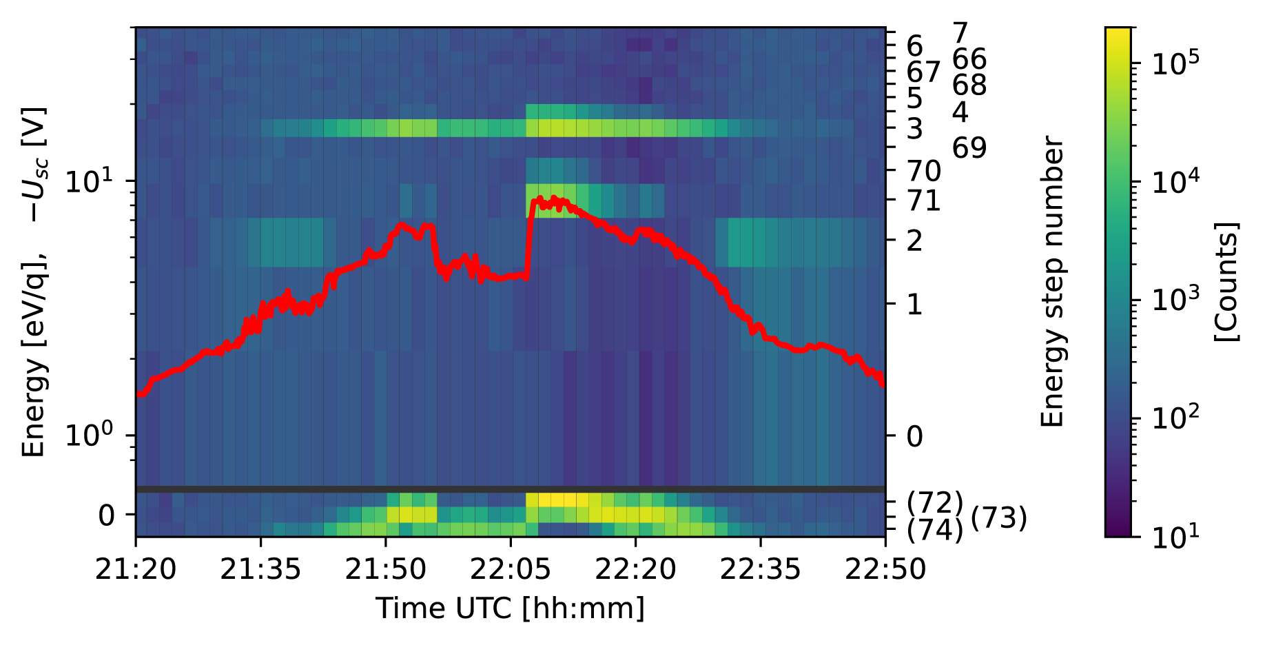
Figure 3 Energy-time spectrogram of positive ions observed in the plasmasphere. The colour scale shows the number of counts observed at each energy step for each time. The energy is given in eV q⁻¹. The value presented is a sum over all directions of arrival and all masses. The red line is an estimate of the negative of the spacecraft potential (in V). The energy step numbers are indicated on the right-side vertical axis. The corresponding tick-marks correspond to the intended energy bin centre, for energy steps 72–74 the intended centre was at 0 eV (bottom of figure).

One immediately notes that the observed signal (colour scale) does not seem to change much with the spacecraft potential. A cold plasma population should be very sensitive to a varying potential and measurements made by the complementary sensor JEI showed a clear correlation with the spacecraft potential (see the accompanying paper by Fraenz et al., 2026). Around 22:10 UTC there are two maxima at about 8 and 15 eV, respectively. Such multiple peaks at different energies are expected for a spacecraft flying through a multi-component cold plasma with a velocity large compared to the thermal velocities of the ions. The ratio of the peak energies would then be equal to the ratio of the masses of the different species in the plasma. In this case, however, the ratio between the peak energies does not match any expected ratio. For example, oxygen ions are 16 times heavier than H⁺, and four times heavier than He⁺. Moreover, the JDC field-of-view does not include the direction of the spacecraft velocity (ram direction).

To understand the observations, we consider the details of the energy sweep performed by JDC, shown in Fig. 4. Each of the blue dots represents one voltage setting on the ESA (right side vertical axis), which corresponds to a particle energy (left side axis). The energy steps occur in groups of three. This is intentional; to reduce the telemetry data volume the number of energy steps reported can be reduced from 75 to 25 by binning three consecutive energy steps together. The idea with the triangular shape of the sweep is that some energies are covered during the first (upgoing) half of the sweep and that the gaps in the energy coverage are filled in during the second (downgoing) half. The advantage with this is that the same range of energies is covered twice in each sweep, giving a time resolution that is twice as high for mid-range energies. The energies for each group of three energy steps are selected such that the upgoing half of the sweep skips over the energies used in the downgoing part of the sweep and vice versa: The upgoing and downgoing part interleave their energy settings. The disadvantage of such a sweeping scheme is that larger voltage steps are necessary between certain energy steps in both the upgoing and downgoing halves of the energy sweep. The science data from the observation in the plasmasphere revealed that the upgoing and downgoing half of the energy sweep were not properly interleaving. The mismatched interleaving of the energy settings resulted in the artificial energy banding structure visible in Fig. 3. This suggested that the wanted voltages (blue dots) are not realized in practice. A possible reason identified was that the sweep pattern necessary to implement the above energy sweep scheme turned out to be outside of the engineering specification of the high voltage power supply for the voltage U_ESA. Fortunately, the energy sweep could be studied in detail in the laboratory.

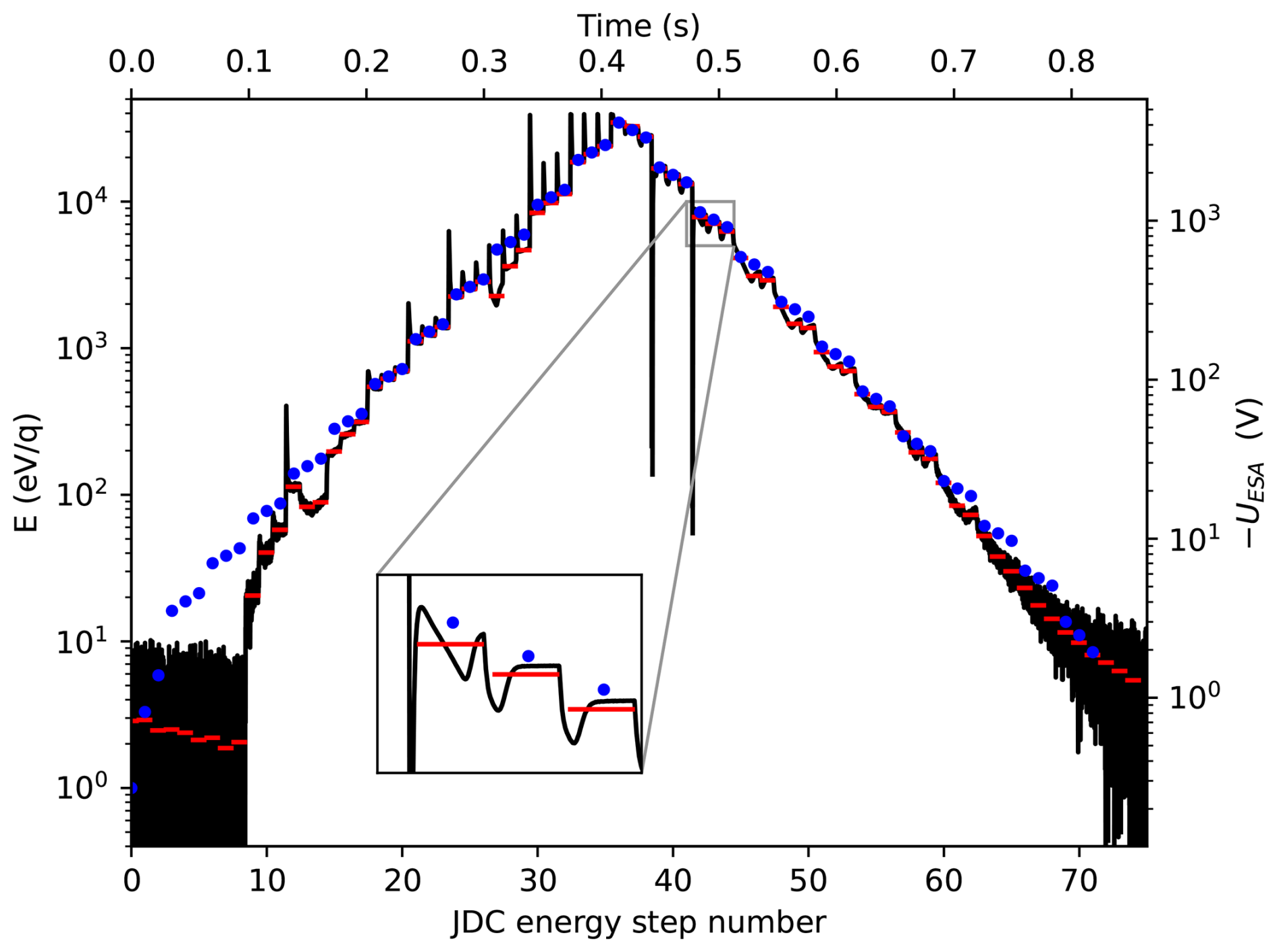
Figure 4 Example of reconstructed electrostatic analyzer voltages. Blue dots mark the intended settings, the black line is the measured voltage and the red dashes are average settings for the time intervals where JDC is recording data. The inset illustrates settling time effects resulting in voltage swings larger than the voltage separation between consecutive energy steps. The intended energy setting for energy steps 72–74 is 0 eV (not shown due to the logarithmic vertical scale). For the final reconstruction of the energy scale, several measurements of this type were combined.

4 Measurements on ground

The flight model of JDC is available on ground. It was replaced on the spacecraft by the flight spare model due to late discovered electrical grounding issues. The two instrument models are very similar and we used the model available on ground to measure the actual voltages on the inner ESA electrode during an energy sweep. Measurements needed partial disassembly and a hardware modification of the instrument, which is one of the reasons why such a measurement was not done with the flying unit before delivery to the spacecraft. The conceptual setup of the measurement is shown in Fig. 1.

Due to the high voltages involved, any measurement has to be done with JDC placed in a vacuum better than 10⁻⁵ mbar. This in turn makes the measurement of a fast changing high voltage waveform a challenge due to the long cables needed to get the signal out of the vacuum tank. A dedicated resistive low capacitance voltage divider was soldered directly to the output of the high voltage power supply for U_ESA. A divider ratio of $\mathrm{R}\mathrm{1}/\mathrm{R}\mathrm{2}=\mathrm{1}\mathrm{G}\mathrm{\Omega }/\mathrm{1}\mathrm{M}\mathrm{\Omega }=\mathrm{1}/\mathrm{1000}$ was used to minimize the additional resistive load to the output of the high voltage power supply. This also allowed to compensate for the cable capacitance of a few 100 pF, while only marginally increasing the capacitive load. The resulting voltage U_M accessible outside of the vacuum system was recorded using a Keysight MSOS204A oscilloscope featuring a 10 bit analogue to digital converter (ADC). 1024 individual recordings were averaged to lower the noise level in the recorded data and to increase the dynamic range. Averaging recordings and further smoothing in time domain resulted in an effective dynamic range of more than 16 bits, sufficient to record the complete voltage sweep in a single measurement.

The results of the measurement of U_ESA are shown as a black solid line in Fig. 4. An obvious feature is the spikes (overshoots), especially on the upgoing part of the sweep. They may look problematic but are in fact not. Each new energy step starts with a 2 ms long deadtime to allow the voltages to settle to their new values. No measurements are made during the deadtime. During the remaining 9.52 ms of each step the measurements are done. The red horizontal dashes in Fig. 4 show the average voltage over the 9.52 ms of measurement for each energy step. In many cases we note a clear deviation between the red line and the corresponding blue dot. Especially the first ten energy steps are strongly affected. It means that the observation at that energy step is not done at the intended energy. As can be seen, by comparing the red lines with the black, the voltage is also not constant during a step. Hence, the effective width of an energy bin will be larger than expected. Energy step numbers below 15 suffer from a significant lag of the obtained voltage when the upgoing part of the sweep starts. The reconstruction of the voltage present in these energy steps has rather large uncertainties and a high variability, making it difficult to reliably reassign an energy value to these steps. The fundamental problem is that the power supply is operated outside of its engineering specification. The output voltage does not settle fast enough for the voltage sweep patterns envisioned. Also, the time required to reach a new target voltage depends on the value of the previous setting. The latter is important especially when reducing the voltage from large to near zero values. This behaviour was not discovered during instrument calibration as calibration at energies below 100 eV is complicated and slow due to difficulties in generating sufficiently stable and intense ion beams at such low energies.

5 Correcting the energy scale

Assuming that the JDC flight spare model on the Juice spacecraft behaves the same way as the model in the laboratory on ground, we can now correct the observations made. Figure 5 presents the energy-time spectrogram of the reconstructed observations. To get the true energies of each step we have used the average values of the voltage applied to the electrostatic analyzer, that is, the red lines in Fig. 4, whenever these are stable and reliable. Sometimes it is not possible to unambiguously determine the voltage during a step and we have then removed the observations made during that step. The energy step numbers corresponding to the different energies are shown on the right side vertical axis. We note that almost all energy steps we have used in this energy range are taken from the downgoing part of the sweep.

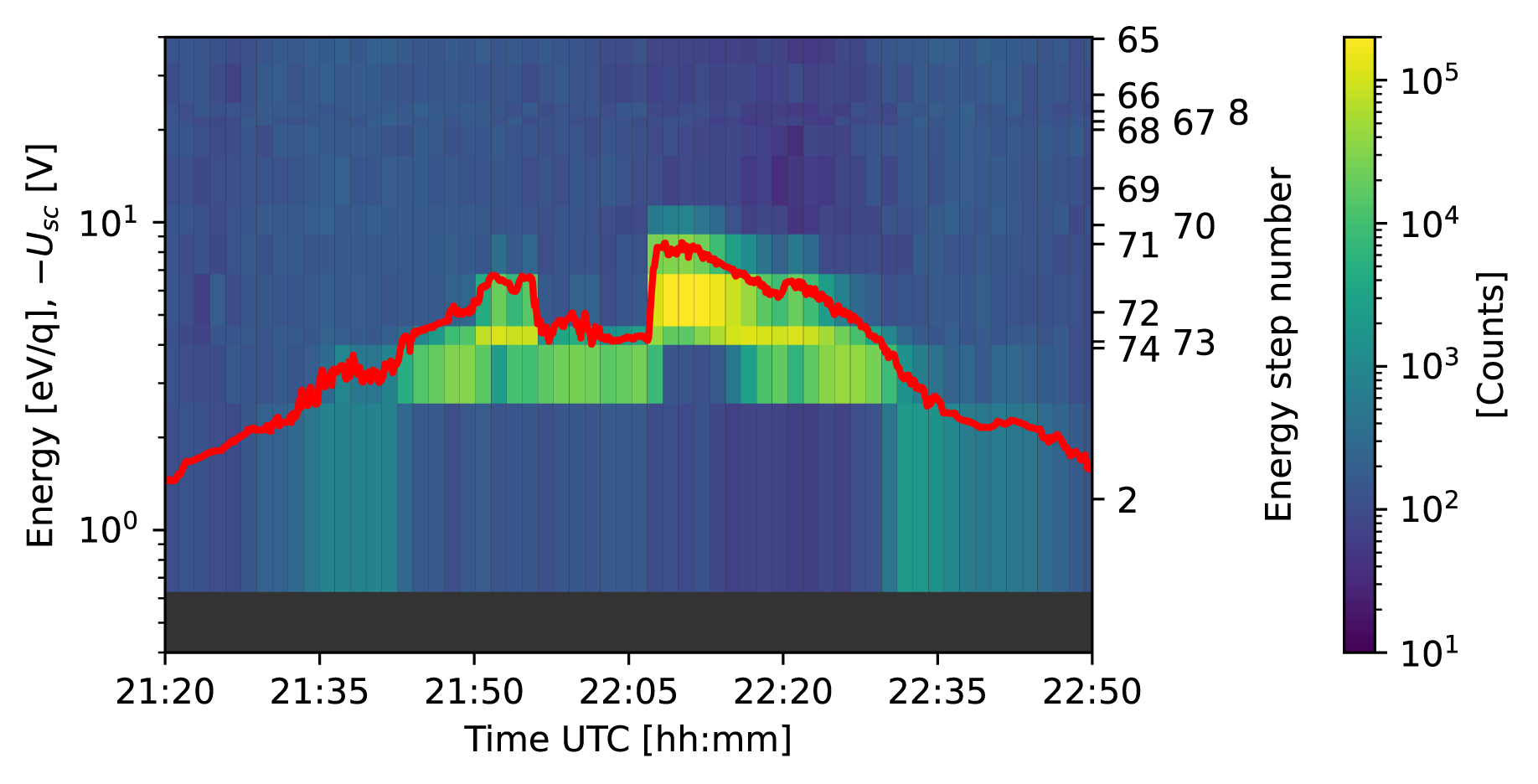
Figure 5 The same energy-time spectrogram as in Fig. 3 after correction of the energy scale. The energy is given in eV q⁻¹. The value presented is a sum over all directions of arrival and all masses. The red line is an estimate of the negative of the spacecraft potential (in V) estimated from RPWI observations. The energy step numbers are indicated on the right-side vertical axis.

We see that the banding of the signal seen in Fig. 3 has now disappeared. The observed counts vary clearly with the estimate of the spacecraft potential as we expect for a cold plasma. It should be stressed that the reconstruction is done based only on the laboratory measurements described in the previous section, without any knowledge about the spacecraft potential. No further adjustments of the data have been made to make the ion observations match the potential. The resulting energy-time spectrogram looks smooth. The observations made on the upgoing and downgoing parts of the energy sweep are now comparable and no artefacts of the sweeping pattern are seen.

The estimated uncertainty of the reconstructed energy levels shown in Fig. 4 (red dashes) is about ±0.5 eV. Measurement uncertainties of U_ESA of about ±50 mV are the most dominant contribution to that. Also, for some energy steps, U_ESA was found to not have stabilized sufficiently within the 2 ms long settling time at the beginning of each energy step; these were removed from the data shown in Fig. 5. The other main source of error are possible differences between the flight spare model of JDC on the spacecraft and the flight model available in the laboratory, estimated to add ±40 mV uncertainty to the value of U_ESA. The uncertainty of the JDC electrostatic analyzer constant $E/U_{\mathrm{ESA}}=\mathrm{7.8}\pm \mathrm{0.1}$ and the energy resolution of $\mathrm{\Delta }E/E=\mathrm{0.15}$ have both a negligible effect on the uncertainty of the corrected energies.

All future observations could be corrected in the same way, but that would mean a sub-optimal use of the instrument. Measurements from some energy steps would have to be excluded from the analysis and the distance between two energy steps would vary. For some energy steps the distance between them would be smaller than the energy resolution, $\mathrm{\Delta }E/E=\mathrm{0.15}$, which is not optimal. In such a case, several energy steps would sample the same energy range. Additionally, we see in Fig. 5 that the energy coverage, especially below 10 eV, is very limited. This is partly a consequence of the behaviour of the sweep voltage, as is seen in Fig. 4, but also a feature of the original energy table. To address the science questions related to low-energy plasma a better coverage over the lowest energies is desired. To resolve all these issues, the original energy table was replaced by three newly designed energy tables with a better performance, which is further discussed in Sect. 7.

6 Simulating the observations

During the passage through the plasmasphere, positively charged ions are accelerated towards a negatively charged spacecraft. The energy change of an ion is $\mathrm{\Delta }W=-q{U}_{\mathrm{sc}}$, where q is the charge of the ion and U_sc the spacecraft potential. An ion originally at rest with respect to the spacecraft will then be observed with an energy equal to ΔW. In certain observation conditions, the low-energy cut-off seen in an energy spectrum can be used to estimate the spacecraft potential (Odelstad et al., 2017; Bergman et al., 2021). In our case, however, we observe most ions at energies below the spacecraft potential. The reason for this is the observation geometry. During the passage through the plasmasphere, JDC looks mostly in the anti-ram direction.

To understand the details of the observations in the plasmasphere and their relation to the estimate of the spacecraft potential, we made a simple model. We assume a point-like spacecraft with a slightly negative spacecraft potential ramming a cold plasma (k_BT=0.1 eV) of constant density. This means in our model the spacecraft is always smaller than the Debye length. This means that the model does not include any effects of the shape of the actual spacecraft. (This is different from the model in Fraenz et al. (2026) where the Debye length was assumed to be small compared to the spacecraft size.) The ram velocity is obtained from the actual spacecraft trajectory and the spacecraft potential is taken from RPWI measurements. We model the plasmasphere as a corotating plasma of O⁺ ions and compute the velocity distribution as seen from the spacecraft for the time interval shown in Figs. 3 and 5.

To comprehend what JDC would observe, we consider Fig. 6, which shows cuts through three-dimensional velocity distributions in the spacecraft frame of reference. Panel (a) is the distribution resulting from a case with a zero spacecraft potential. There is only a shift with the ram velocity present. If we add a negative spacecraft potential, the positive ions are accelerated from all directions towards the spacecraft gaining energy. In panel (b) we see how this acceleration “blows up” the velocity distribution into a circular shape. The white arc indicates the JDC field-of-view. The boresight of the sensor is 45 deg to the anti-ram direction. This means that JDC cannot observe the ram flux directly. However, as soon as the spacecraft potential becomes sufficiently negative (as in panel b) it can overcome the ram velocity and attract positive ions towards the spacecraft, also from the anti-ram direction.

By empirically selecting a part of the JDC field of view and integrating over the solid angle of this part, we obtain a simulated observed energy spectrum for the whole passage through the plasma sphere (Fig. 7). The selected part of the field of view included was chosen to best match the observations.

We note that the simulated spectrum reproduces the key features of the corrected observed spectrum (Fig. 5). The energy where the maximum flux is observed varies with the spacecraft potential. As the observation is done in the anti-ram direction, the detected signal is also observed at energies (in eV) below the negative of the spacecraft potential (in V). Additionally, it should be pointed out that the absence of flux at the lowest energies for part of the time interval is recreated by the simple model. The size of these “holes” depends on the assumed ion temperature. A warmer ion population would give raise to fluxes in a less defined energy range and less clear “holes”. The appearance also depends on over how large solid angle the integration is made. For simplicity we consider the ram direction always to be in +x direction relative to the spacecraft and we do not consider the change in the ram velocity vector direction during the flyby. Our model uses O⁺ ions only. For lighter ions like H⁺ or He⁺, the ram energy is smaller and the energy gain due to the spacecraft potential dominates. For the given observation geometry, these ions will appear in the energy spectrum at higher energies closer to −qU_sc. A preliminary analysis of the JDC mass matrices shows a significant presence of both H⁺ and O⁺. At energies below 1–2 eV, the true shape of the spacecraft significantly affects the trajectories of particles reaching the detector. The point-like spacecraft used in our model cannot reproduce these effects and model results likely differ from observations. Some of the choices we made are arbitrary and the model is very simple but still it is sufficient to qualitatively explain the JDC observations.

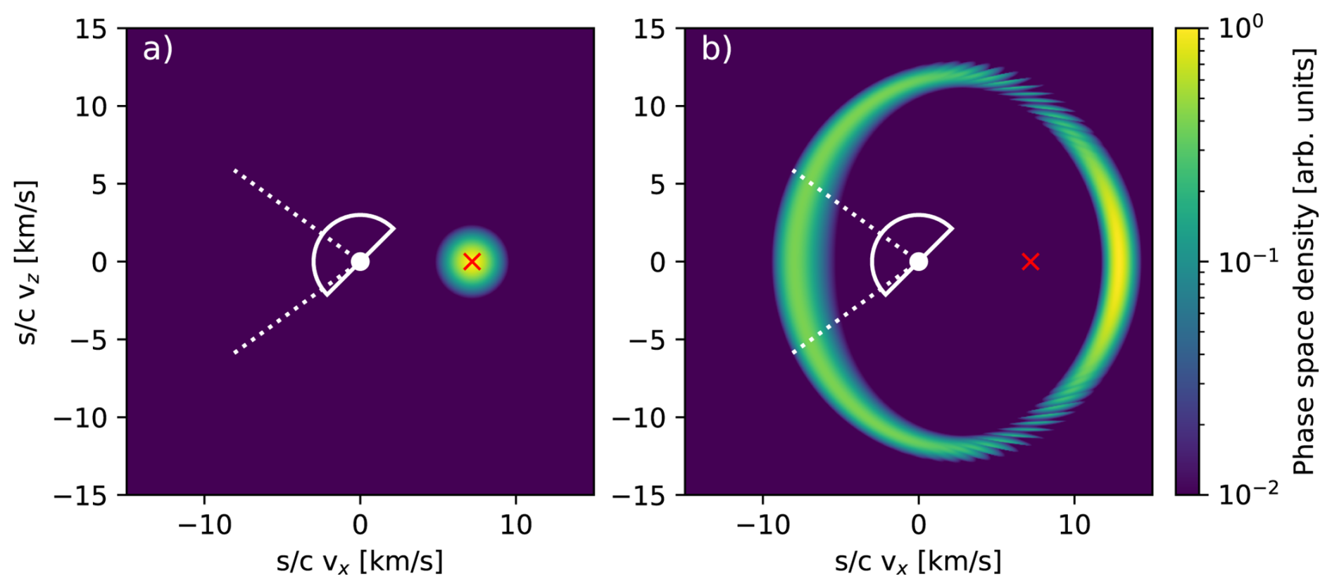
Figure 6 Example oxygen velocity distribution functions. The red cross indicates the ram velocity of 7.1 km s⁻¹. The spacecraft potential in the simulations is set to (a) 0 V and (b) −8.9 V. The JDC field-of-view is indicated with a white arc, dashed lines indicate what part of the distribution was integrated to obtain an energy spectrum. The thin stripes visible in part of the ring are a simulation artifact.

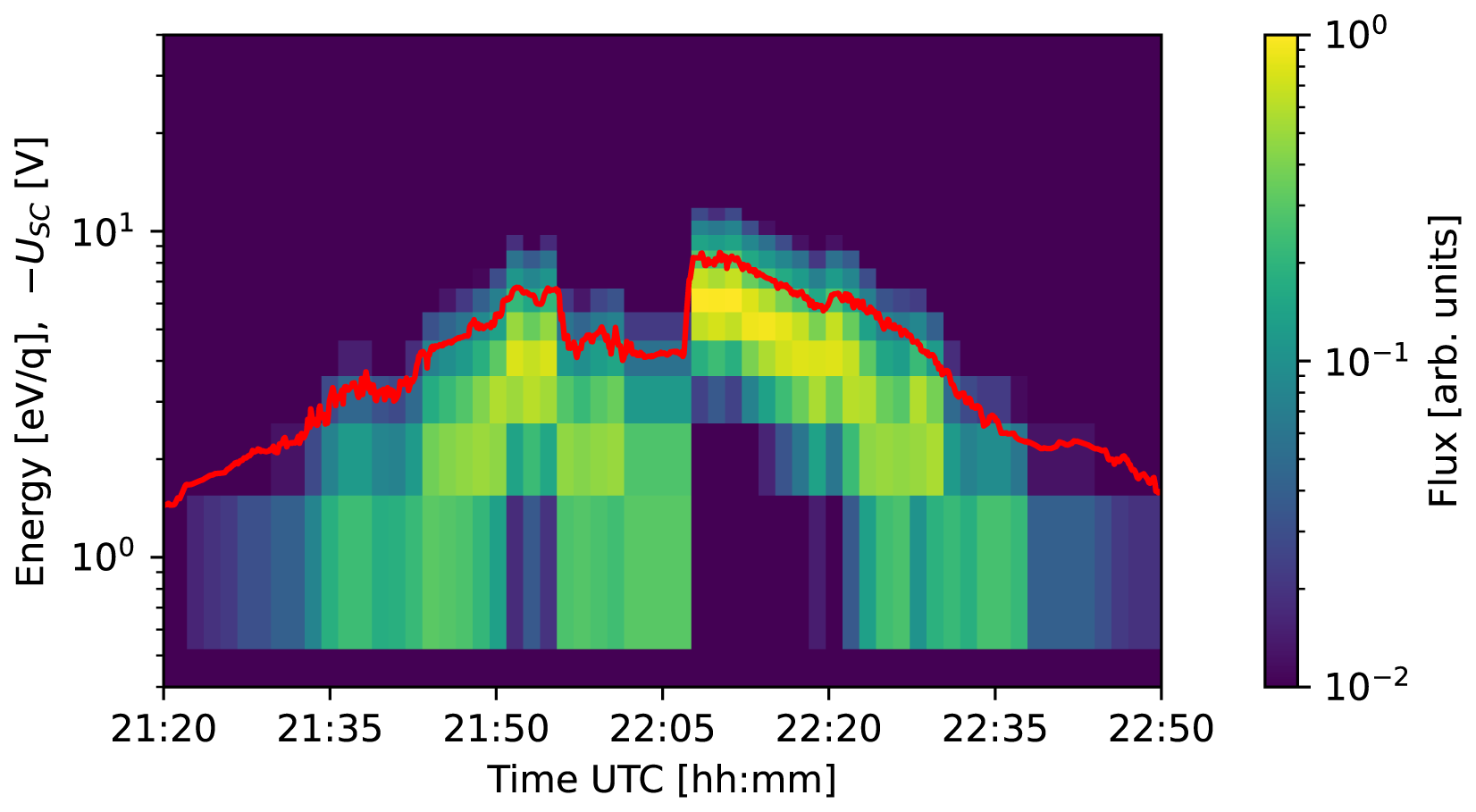
Figure 7 Simulated energy-time spectrogram for JDC measurements in the plasmasphere, assuming an oxygen ion plasma with a temperature of 0.1 eV.

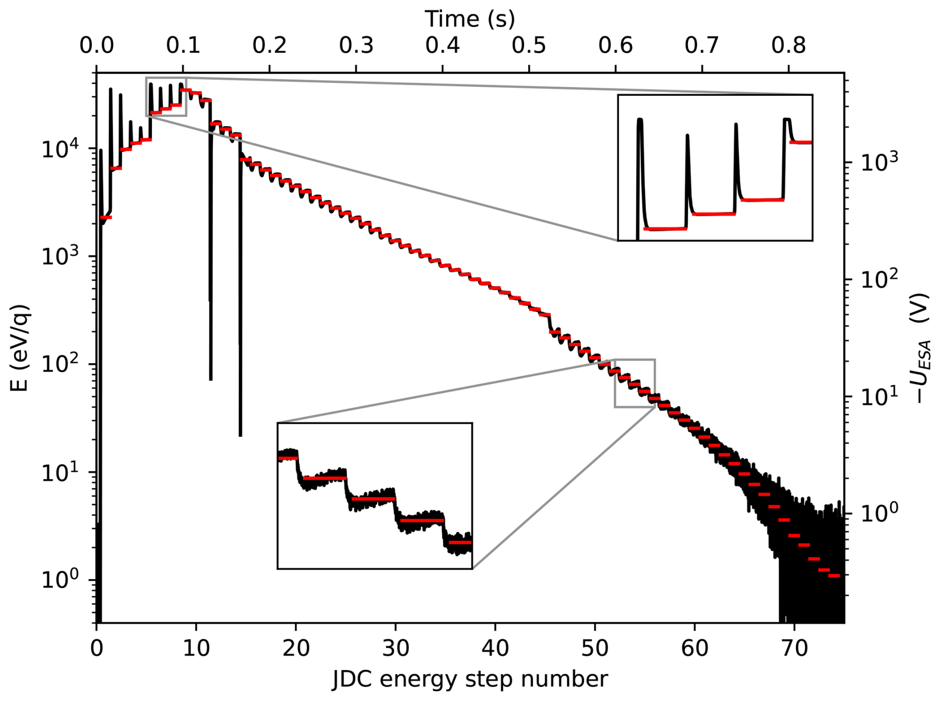
Figure 8 Optimized energy table for the 1 eV to 35 keV range. The other new tables use the same approach with a long and slow downgoing part of the sweep. The step visible at energy bin number 45 is due to a range change in the high voltage power supply.

7 Optimizing future measurements

From Fig. 4 it is clear that the energy sweep does not optimize the observations, especially not at low energies. Therefore, we constructed a different energy sweep, which was extensively tested on ground and found to work reliably. A measurement of the ESA voltage of the laboratory model using the resulting sweep table is shown in Fig. 8. The red horizontal dashes are the average energy/voltage during each energy step and the black solid line is the measurement of the sweep voltage, obtained as described in Sect. 4. Energy steps 0, 1, and 2 are designated sacrificial energy steps, where no stabilized voltages are required. These energy steps are used to raise the voltage as quick as possible to kV levels. After reaching the peak energy setting in step 10, voltages are reduced as slowly as possible down to their minimum setting in energy step 74. The new sweep strategy gives an even distribution of energy steps over the desired energy range. As can be seen from the insets in Fig. 8, the voltage is now stable during each step and any occurring spikes are short enough not to affect the measurements. The updated sweep table still enables down-binning from 75 to 25 energy bins when needed. The only advantage with the triangular sweep that had to be given up is the higher time resolution of the mid-energy range.

The general software update of the PEP instrument performed in February 2026, provided an opportunity to implement this change but also to add two additional energy sweep tables. The Juice mission provides a challenge for particle measurements, probing many different plasma environments. The six different sensors comprising PEP are designed to complement each other. JDC (together with JEI at the other side of the spacecraft) cover the mid-energy regime (∼1 eV q⁻¹–35 keV q⁻¹) and must be able to detect heavy ions (e.g., O⁺, S²⁺, O²⁺) in the Jupiter magnetosphere, with energies up to tens of keV (Allegrini et al., 2022) as well as ionospheric plasma at Ganymede with energies below 10 eV (Frank et al., 1997; Valek et al., 2022). The observed energies of cold ionospheric ions depend on the ram velocity as well as the spacecraft potential. Heavier ions will be detected at higher energies than lighter ions. The Juno flyby of Ganymede in June 2021 suggests that an energy range of a few eV to a few hundred eV is a good choice for ionospheric observations (Valek et al., 2022). To better meet the challenges of a varying environment, we introduced a energy table focused on low-energy ion observations. This was partly motivated by the successful introduction of dedicated low-energy tables for RPC-ICA on Rosetta (Stenberg Wieser et al., 2017). A dense energy coverage of the lowest energies (that is, no gaps in energy coverage between different energy steps) revealed a highly dynamical cometary ion population at energies below 60 eV. In the Rosetta case, the new table also meant increasing the time resolution from 192 to 4 s, by turning off the elevation sweep. The improved properties came with a price: the energy range was reduced to cover from only a few eV to 85 eV. Observations made using this energy table gave unique insights in the dynamics of the cold ions close to the comet nucleus (e.g. Bergman et al., 2021; Yun et al., 2026). It also provided an independent observation of the spacecraft potential, which could be used to cross-calibrate the ion spectrometer with the Langmuir probe instrument onboard (Odelstad et al., 2017).

The new energy tables for JDC cover 1 eV–35 keV, 1 eV–18 keV and 1–500 eV. The energy table with the maximum energy of 35 keV replaces the old defective table. It has the maximum energy coverage possible for JDC, but uses corrected low-energy settings. A new energy table with an maximum energy of 500 eV was created and optimized for ionospheric measurements close to the icy moons. The energy table with the maximum energy of 18 keV is an engineering compromise with reduced power consumption while still providing reasonable high energy coverage and improved low-energy coverage. Such a table may give the opportunity to run JDC even when the power available is limited and hence increase the science return.

The sweep pattern of each table variant was validated using the measurement scheme shown in Fig. 1. Focus was put on reliably reaching both the highest and lowest energy settings within a single energy sweep, while not exceeding the speed capabilities of the high voltage power supply and while keeping the spacing between the individual energy steps as regular as possible. All three energy tables follow the same design idea as shown in Fig. 8, but with different maximum energy settings. The table for the lowest energy range aims to achieve an as dense coverage at the lowest energies as possible. The improved coverage below 100 eV for all three new tables is shown in Fig. 9. While the figure illustrates the improved coverage for positive ions, the same coverage improvement is also available for electrons and negative ions when JDC is configured to measure negatively charged particles.

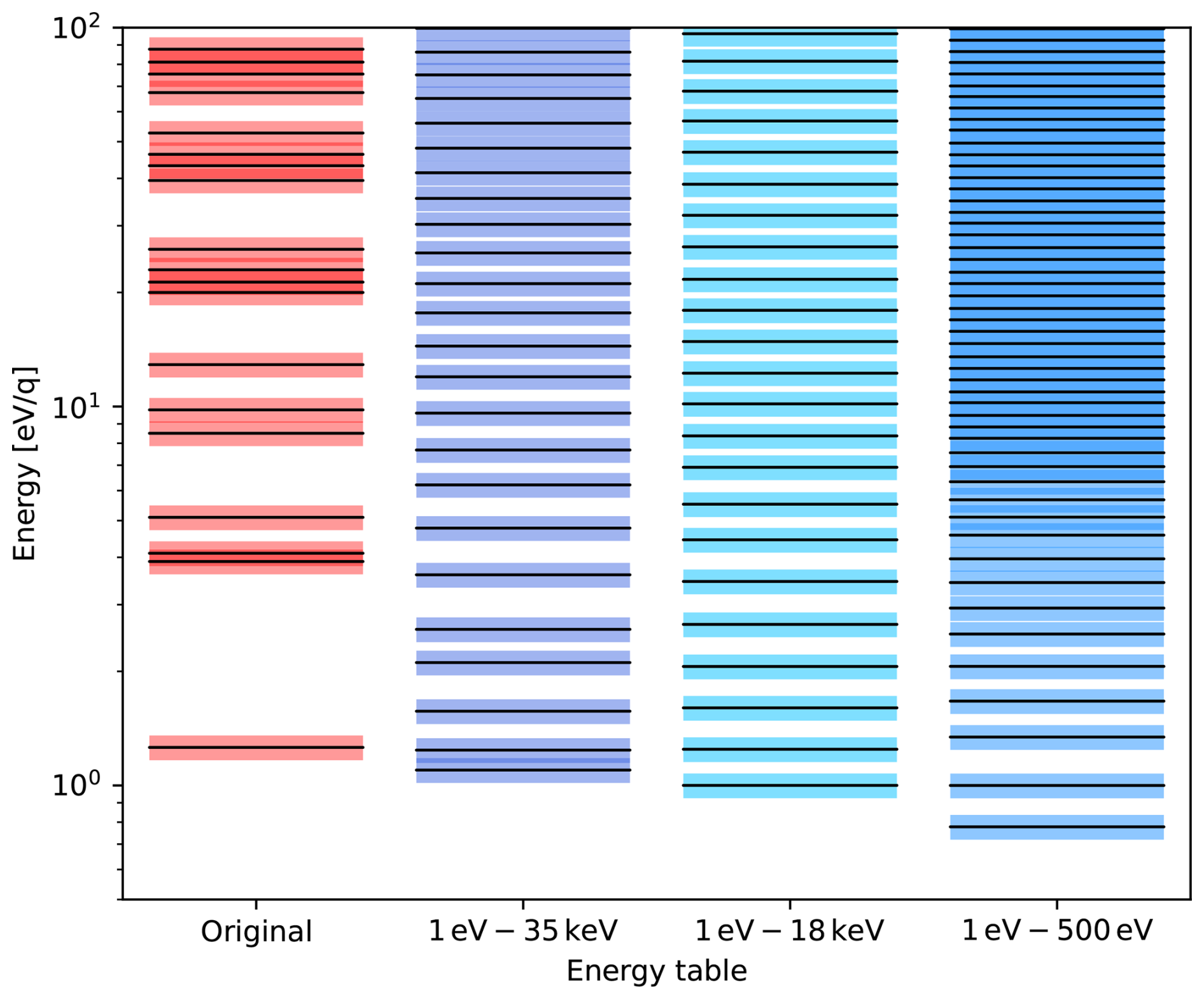
Figure 9 Energy step placements. Original (left, red), new tables (blue shades). Black lines indicate the centre energy of each bin, coloured areas the energy coverage of each bin. Only minimal irregularities for the new tables remain.

The present analysis has important implications for the forthcoming JDC measurements at Jupiter's icy moons. During many of the flybys of Callisto, Ganymede and Europa, JDC will ram into the ionosphere, either inbound or outbound. The spacecraft will likely become negatively charged close to Ganymede and Europa and the new tables offer better tools to characterize the positive ions in the moons' ionospheres. Due to the low orbital speed of Juice during the orbital phase around Ganymede, the spacecraft potential will be the main driver of ionospheric ion collection. Close to Callisto, the spacecraft will likely be positively charged, and the spacecraft potential will be the main driver of ionospheric electron collection. In both cases the three new tables will significantly improve data collection at low particle energies and offer flexibility in operation planning.

8 Summary and conclusions

We used data recorded by Juice in the Earth's plasmasphere to assess the performance of the Jovian Plasma Dynamics and Composition analyzer (JDC), especially at low ion energies. By combining the sensor's observations in space with measurements made in the laboratory, we could interpret the observations and correct the existing energy sweep table. Based on the results we constructed new energy sweep tables for JDC to optimize low-energy ion observations at the final destination.

Our study shows the importance of in-flight calibrations. On ground calibrations of the sensor response to low-energy ions are extremely difficult and usually not done (Wuest et al., 2007). Thus, for particle detectors, operations during planetary flybys are important as they give access to multiple populations besides the mono-energetic and highly directional solar wind. An electrically charged spacecraft attracts ions of the opposite charge and enables measurements down to the lowest energies. If the spacecraft potential also varies with time, observations of a cold plasma (e.g., the plasmasphere) provide a dataset enabling calibration over a range of energies below 10 eV.

To interpret the data observed in space, we made use of a copy of the flying instrument that is available on ground. The combination of actual space data and laboratory measurements is very powerful. It requires that the instrument model on ground is, or can be made, sufficiently comparable to the flying model. If this cannot be realized, a detailed characterization of the energy sweep has to be done before launch on the flight model. To optimize low-energy ion observations, this is recommendable, even if the observations are complicated and modifications to the hardware have to be made.

In summary, in-flight calibrations are extremely important to maximize science return, especially concerning low-energy ion observations. To be able to support the calibrations with laboratory measurements on a copy of the instrument is highly valuable.