Harmonic content of Ap index

Fourier spectral analysis is applied to the planetary geomagnetic index Ap for the February 2001, 2003, and 2017 time intervals. We investigate how Fourier coefficients change in time with respect to geomagnetic activity. A detailed analysis of the 13–14 February 2001 substorm revealed that higher harmonics were suppressed during the event, contrary to what was expected.

1 Introduction

Geomagnetic indices Kp and Ap, introduced by Bartels (1949, 1957), provide a widely used measure of magnetospheric convection strength (e.g., Thomsen, 2004; Rowland and Wygant, 1998; Wang et al., 2025). Large-scale magnetospheric convection is driven by day- and night-side magnetic reconnection (Siscoe and Huang, 1985; Cowley and Lockwood, 1992; Dai et al., 2024; Zhu et al., 2024, 2025, etc.) and penetrates deep into the inner magnetosphere (e.g., Wygant et al., 1998; Dai et al., 2015; Thaller et al., 2015). Abe et al. (2023) compared the spectral content of geomagnetic indices and the Sunspot Number (SSN) during solar cycles 23 and 24. Zajtsev et al. (1993) and De Michelis et al. (2014) considered Fourier spectra of the geomagnetic field. Rangarajan and Lyemori (1997) analyzed data on the Kp and Ap indices from 1932 to 1960 and found that the relative frequencies of Kp with different magnitudes show consistent seasonal and solar-cycle dependencies. de Gonzalez et al. (1993) investigated a different set of Ap data using the power spectrum technique. The monthly Ap power spectrum reveals a period around 4 years, associated with a double peak structure in geomagnetic activity. Daily Ap spectrum peaks are interpreted as harmonics of a 6-month period, and others as linked to solar rotation periodicity, suggesting the juxtaposition of two Fourier sequences.

Another geomagnetic index, Dst, better describes the intensity and position of the ring current, which influences the H-component of the Earth's surface geomagnetic field. Le Mouel et al. (2019) identified several significant spectral components in Dst data using singular spectrum analysis, namely a prominent 6-month component, along with 47, 10.6, 1, 22, 11 and 5.5 year components. Rigozo et al. (2006) applied spectral analysis to the annual and monthly average series of Ap from 1868 to 2001. Riabova and Spivak (2018) used a similar approach to the data from the Mikhnevo Geophysical Observatory in 2009–2015. Riabova (2018) developed a wavelet model for analyzing geomagnetic field variations, which demonstrated effectiveness in detecting sudden commencements.

The study of Pai and Sarabhai (1964) examines periodic fluctuations in the Earth's magnetic field during magnetic storms using data from 1958. Autocorrelation analysis reveals a common 40 min period for fluctuations, primarily during geomagnetic storms. Cliver et al. (1996) proposed that changes in geomagnetic activity associated with alternating sunspot maxima are primarily driven by solar variations, including stronger 27 d recurrent solar wind streams.

Zajtsev et al. (1993) applied fast Fourier transform (FFT) (Cooley et al., 1969) of the magnetic field components measured by a particular magnetic observatory. They reported that some patterns could be recognized in the contour plots of the Fourier coefficients versus time for different phases of substorms.

We present the Fourier decomposition of the Ap index for the February 2001, 2003, and 2017 periods. We focus on changes in spectral content during increased geomagnetic activity. The next section describes the method used in this work. The results are presented in Sect. 3. Finally, a discussion and conclusions are given in Sect. 4.

2 Method

We consider the Ap index as a function of time that can be decomposed into the Fourier sum with the fundamental angular frequency $\mathit{\omega }=\frac{\mathrm{2}\mathit{\pi }}{T}$, where the period is T=27 d. The index is calculated per three hour time interval, that is, the data in $K=\mathrm{27}\cdot \mathrm{8}=\mathrm{216}$ intervals are used. Consider the function Ap(t) in the time interval $\left[\frac{l}{K}T,\frac{l}{K}T+T\right]$ where l≥0 is an integer, and introduce a function Ap_l(t^′) defined for $t^{\prime }\in \left[-\frac{T}{\mathrm{2}},\frac{T}{\mathrm{2}}\right]$ by

$$\begin{array}{}\text{(1)}& {\mathrm{Ap}}_l\left(t^{\prime }\right)=\mathrm{Ap}\left[t^{\prime }+\left({\displaystyle \frac{l}{K}}+{\displaystyle \frac{\mathrm{1}}{\mathrm{2}}}\right)T\right].\end{array}$$

The function Ap_l(t^′) is then approximated by a finite Fourier series

$$\begin{array}{}\text{(2)}& \begin{array}{rl}{\mathrm{Ap}}_l\left(t^{\prime }\right)& =a_{\mathrm{0}l}+\sum _{n=\mathrm{1}}^N\left(a_{nl}\cos n\mathit{\omega }{t}^{\prime }+b_{nl}\sin n\mathit{\omega }{t}^{\prime }\right)\\ & =c_{\mathrm{0}l}\cos {\mathit{\varphi }}_{\mathrm{0}}+\sum _{n=\mathrm{1}}^N{c}_{nl}\cos n(-{\mathit{\varphi }}_{nl}/n+\mathit{\omega }{t}^{\prime }).\end{array}\end{array}$$

Introducing discrete values $t_{lk}^{\prime }=t_k-\left(\frac{l}{K}+\frac{\mathrm{1}}{\mathrm{2}}\right)T$, Ap(t_k)=Ap_k, $t_k=\frac{k}{K}T$, the coefficients a_nl, b_nl, c_nl, and phases ϕ_nl are calculated as follows:

$$\begin{array}{}\text{(3)}& {\displaystyle }{a}_{\mathrm{0}l}={\displaystyle \frac{\mathrm{1}}{K}}\sum _{k=l}^{l+K}{\mathrm{Ap}}_k-{\displaystyle \frac{\mathrm{1}}{\mathrm{2}K}}\left({\mathrm{Ap}}_l+{\mathrm{Ap}}_{l+K}\right),\text{(4)}& {\displaystyle }\begin{array}{rl}{a}_{nl}& =\sum _{k=l}^{l+K-\mathrm{1}}\left[{\displaystyle \frac{K}{\mathrm{2}{n}^{\mathrm{2}}{\mathit{\pi }}^{\mathrm{2}}}}({\mathrm{Ap}}_{k+\mathrm{1}}-{\mathrm{Ap}}_k)(\cos n\mathit{\omega }{t}_{l,k+\mathrm{1}}^{\prime }-\cos n\mathit{\omega }{t}_{l,k}^{\prime })\right.\\ & \left.+{\displaystyle \frac{\mathrm{1}}{n\mathit{\pi }}}({\mathrm{Ap}}_{k+\mathrm{1}}\sin n\mathit{\omega }{t}_{l,k+\mathrm{1}}^{\prime }-{\mathrm{Ap}}_k\sin n\mathit{\omega }{t}_{l,k}^{\prime })\right],n>\mathrm{0},\end{array}\text{(5)}& {\displaystyle }\begin{array}{rl}{b}_{nl}& =\sum _{k=l}^{l+K-\mathrm{1}}\left[{\displaystyle \frac{K}{\mathrm{2}{n}^{\mathrm{2}}{\mathit{\pi }}^{\mathrm{2}}}}({\mathrm{Ap}}_{k+\mathrm{1}}-{\mathrm{Ap}}_k)(\sin n\mathit{\omega }{t}_{l,k+\mathrm{1}}^{\prime }-\sin n\mathit{\omega }{t}_{l,k}^{\prime })\right.\\ & \left.-{\displaystyle \frac{\mathrm{1}}{n\mathit{\pi }}}({\mathrm{Ap}}_{k+\mathrm{1}}\cos n\mathit{\omega }{t}_{l,k+\mathrm{1}}^{\prime }-{\mathrm{Ap}}_k\cos n\mathit{\omega }{t}_{l,k}^{\prime })\right],n>\mathrm{0},\end{array}\text{(6)}& {\displaystyle }{c}_{\mathrm{0}l}=\left|a_{\mathrm{0}l}\right|,\text{(7)}& {\displaystyle }{c}_{nl}=\sqrt{a_{nl}^{\mathrm{2}}+b_{nl}^{\mathrm{2}}},n>\mathrm{0}\text{(8)}& {\displaystyle }{\mathit{\varphi }}_{\mathrm{0}l}=\mathrm{0},a_{\mathrm{0}l}>\mathrm{0}\text{(9)}& {\displaystyle }{\mathit{\varphi }}_{\mathrm{0}l}=\mathit{\pi },a_{\mathrm{0}l}<\mathrm{0}\text{(10)}& {\displaystyle }{\mathit{\varphi }}_{nl}=\arctan (a_{nl},b_{nl}),n>\mathrm{0},\end{array}$$

where arctan of two arguments returns values in the full range [0,2π) and reduces to ordinary $\arctan \frac{b_{nl}}{a_{nl}}$ for $a_{nl}>\mathrm{0},b_{nl}\ge \mathrm{0}$. Here, c_nl are the amplitudes of the particular harmonics and ϕ_nl are their phases, while a_nl and b_nl are Fourier coefficients. The coefficient a_0l is calculated via integration

$$\begin{array}{}\text{(11)}& a_{\mathrm{0}l}={\displaystyle \frac{\mathrm{1}}{T}}\underset{-T/\mathrm{2}}{\overset{T/\mathrm{2}}{\int }}{\mathrm{Ap}}_l\left(t^{\prime }\right)\mathrm{d}{t}^{\prime }\end{array}$$

Because the function Ap_l defined earlier is known only at times separated by three hours, we use linear interpolation, and the integration (11) becomes the sum of 216 areas of the corresponding trapezoids in (3). The summation is over k from k=l which corresponds to $t^{\prime }=-T/\mathrm{2}$, to $k=l+K$ which corresponds to $t^{\prime }=T/\mathrm{2}$. The area of the trapezoid determined by two points Ap_k and Ap_k+1 is $({\mathrm{Ap}}_k+{\mathrm{Ap}}_{k+\mathrm{1}})T/\left(\mathrm{2}K\right)$. All Ap_k appear twice, except the very first and the last in the sum, which appear only once.

Similarly, the coefficients a_nl and b_nl in (4) and (5) are calculated by integrations

$$\begin{array}{}\text{(12)}& {\displaystyle }{a}_{nl}={\displaystyle \frac{\mathrm{2}}{T}}\underset{-T/\mathrm{2}}{\overset{T/\mathrm{2}}{\int }}{\mathrm{Ap}}_l\left(t^{\prime }\right)\cos n\mathit{\omega }{t}^{\prime }\mathrm{d}{t}^{\prime },\text{(13)}& {\displaystyle }{b}_{nl}={\displaystyle \frac{\mathrm{2}}{T}}\underset{-T/\mathrm{2}}{\overset{T/\mathrm{2}}{\int }}{\mathrm{Ap}}_l\left(t^{\prime }\right)\sin n\mathit{\omega }{t}^{\prime }\mathrm{d}{t}^{\prime },\end{array}$$

which again results in sums with respect to k. The difference is that now each element of the sums is not simply the trapezoid area but the actual integral of the linearly interpolated Ap_l(t^′) multiplied by cos nωt^′ or sin nωt^′ in a time interval of three hours. The interpolation is given by

$$\begin{array}{}\text{(14)}& {\mathrm{Ap}}_l\left(t^{\prime }\right)={\mathrm{Ap}}_k+{\displaystyle \frac{{\mathrm{Ap}}_{k+\mathrm{1}}-{\mathrm{Ap}}_k}{T}}\left(t^{\prime }+{\displaystyle \frac{T}{\mathrm{2}}}\right),t^{\prime }\in \left[-{\displaystyle \frac{T}{\mathrm{2}}},{\displaystyle \frac{T}{\mathrm{2}}}\right].\end{array}$$

Both c_nl and ϕ_nl depend on two indexes, in frequency and in time. The step along l corresponds to three hours in time, while a step along n means an increase in frequency by ω. In other words, all coefficients and phases are calculated in (3)–(5) for every three-hour interval. We use Ap data of 27 days. N was set equal to $K/\mathrm{2}=\mathrm{108}$. For any particular time, t, which is determined by $k=t/\mathrm{3}$, time in hours, k in three-hour intervals from the beginning of the year, the allowed values of l are in the range $[k-\mathrm{215},k-\mathrm{1}]$, and the allowed starting time of t is in the range $[\mathrm{3}k-\mathrm{645},\mathrm{3}k-\mathrm{3}]$. On the other hand, for a given l, there is only one set of coefficients a_nl and b_nl.

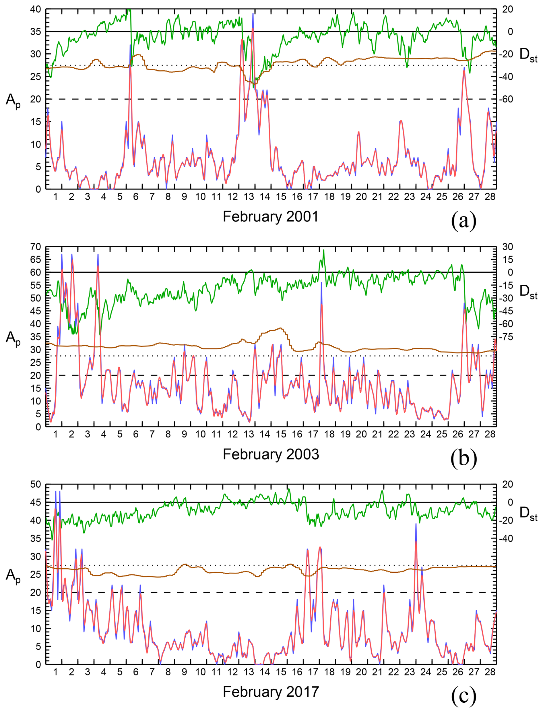
Figure 1 Ap time profiles for our three time periods. The blue lines represent the original data, but they are mostly obscured by the red lines showing the reconstructed Ap. The dashed horizontal lines indicate Ap = 20 nT. Dst index is drawn by the green lines in the top part of the panels, with the scales on the right hand side and the horizontal solid lines indicating Dst = 0 nT. The brown lines in the middle part of the panels are explained in the text.

3 Results

The time profiles of the Ap index for the Februaries 2001, 2003 and 2017 are shown in Fig. 1. The intervals contain relatively long quiet periods, with Ap<20 nT, and strong disturbances with Ap up to 60 nT. The graphs are supplemented by profiles of the Dst index.

The Fourier harmonics with N=108 work very well for February 2001, as one can see from Fig. 1a. The original data and the reconstructed Ap are practically indistinguishable for most of the month. The reconstruction is done in the following way. For a given time t, the closest t_k is found that t≤t_k. The interval $\left[\frac{l}{K}T,\frac{l}{K}T+T\right]$, for which the coefficients a_nl and b_nl are calculated, is centered at t_k. This specifies the value of l: $l=k-\frac{K}{\mathrm{2}}$. Then a_nl and b_nl are determined from Eqs. (3)–(5) and the reconstructed Ap(t) from Eqs. (1)–(2).

The month of February 2001 was relatively quiet, with Ap_max=40 nT, without abrupt peaks. On the other hand, February 2003 was a very disturbed month, with Ap_max=70 nT, and rapid transitions from nearly smooth behavior changed to abrupt jumps. The reconstruction follows the data very well, but some minor deviations can be seen from time to time. February 2017 was a relatively quiet month. The reconstructed and real data are very close to each other.

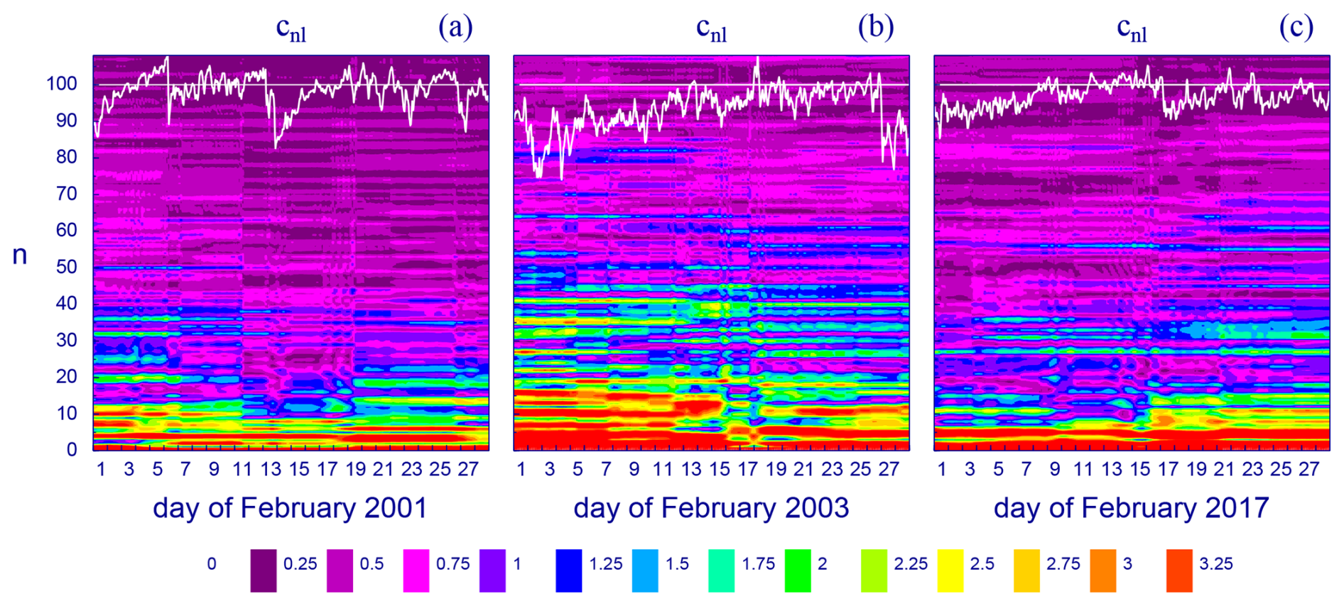
Figure 2 Contour plots of c_nl for our three periods under consideration. They are supplemented by Dst profiles in the top parts as the white lines. The Dst values are in arbitrary units but their scales are identical and the white horizontal lines indicate a zero value.

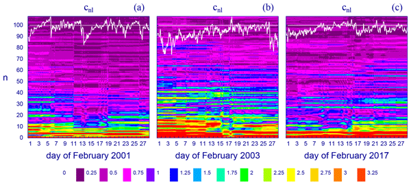
The two-dimensional functions c_nl and ϕ_nl can be represented as contour plots. The contour plots of c_nl for our three periods are shown in Fig. 2. In the contour plots, the horizontal axis represents time, and the vertical axis represents n. The angular frequency ω_n and n are related as ω_n=nω. For example, n=10 corresponds to frequency 103 µHz. The l is associated with time as has been described above. It can be seen that maximum intensities occur at low frequencies. As frequency increases, the value of c_nl decreases. Fig. 2 shows the pronounced structure at the lower frequency components, probably associated with atmospheric tides (Chen et al., 2024).

Raw magnetic data typically show atmospheric tides at diurnal and semi-diurnal periods, corresponding to n=27 and n=54. The effect is especially pronounced in February 2017 and 2003; there are clear lines in the lower frequencies. February 2001 was more active, and the atmospheric tide effects were weaker. This means that geomagnetic activity covers the magnetic signatures of atmospheric tides and also planetary waves (at lower n), which are visible in the Ap time series. The disappearance of tidal signals in Ap indicates geomagnetic activity.

Figure 3 Contour plots of modified and normalized ϕ_nl.

Figure 4 Profiles of modified and normalized ϕ_nl for three n in February 2001.

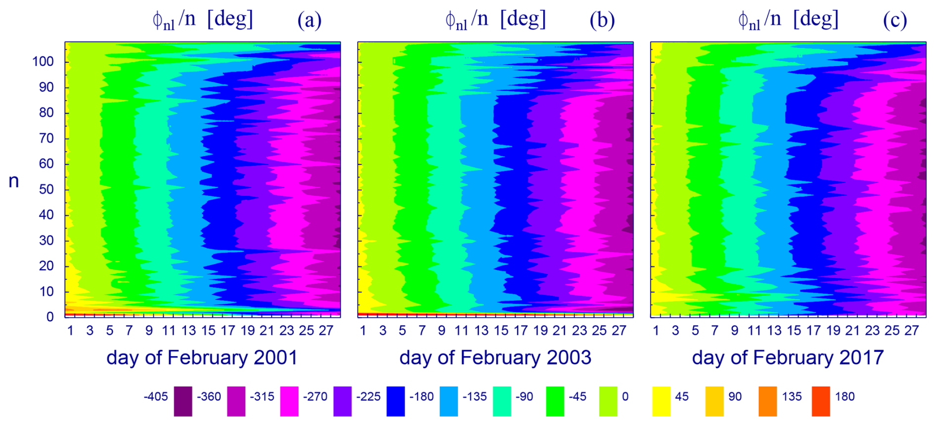
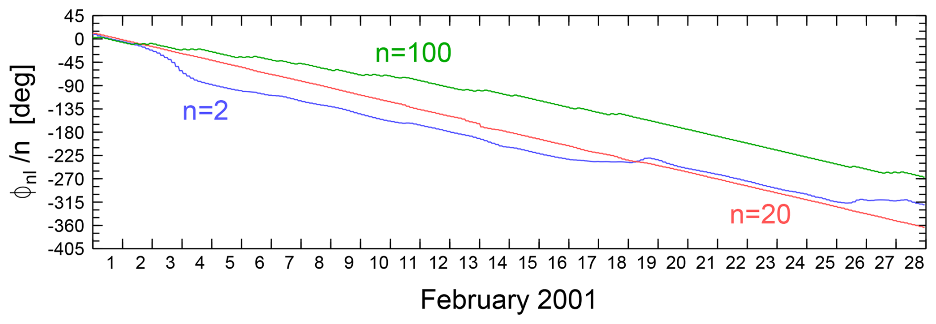
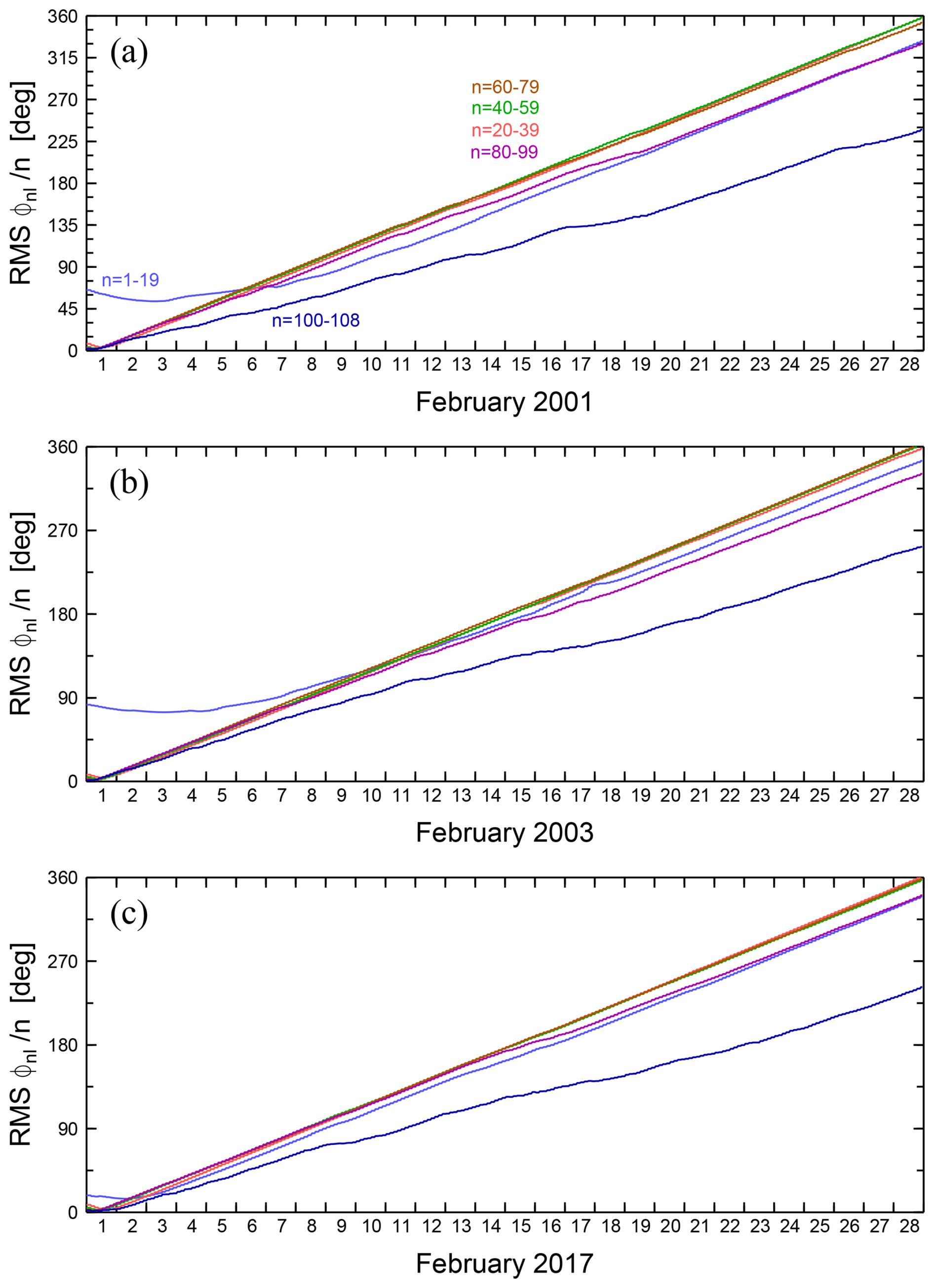
Figure 5 Profiles of RMS of modified and normalized ϕ_nl for six bands of n, distinguished by colors. Color-coding of parts (b) and (c) is the same as of (a).

The contour plots of the modified and normalized phase ϕ_nl are demonstrated in Fig. 3. Eqs. (8)–(10) yield values between 0 and 360°. The ϕ_nl was modified to make it continuous (by adding or subtracting a multiple of 360°). Consequently, ϕ_nl was normalized by division by n (it appears in this form in Eq. 2). The contour plots show that modified and normalized ϕ_nl decreases nearly monotonically over time. And Fig. 4 shows that this decrease is nearly linear. Deviations from the linear trend are observed during periods of increased geomagnetic activity. For example, in February 2017, a relatively quiet period, most normalized and modified ϕ_nl are straight lines. Figure 5 displays the root mean square (RMS) of modified and normalized ϕ_nl for selected frequency bands. During the solar maximum (2001, 2003), the band 1–19 hits 90° in the beginning, whereas during the relatively quiet period (2017) it hits 0° in the beginning. The other bands of the phase angles show similar temporal profiles, hitting nearly 0° in the beginning.

Figure 6 Hodographs of the complex Ap^c.

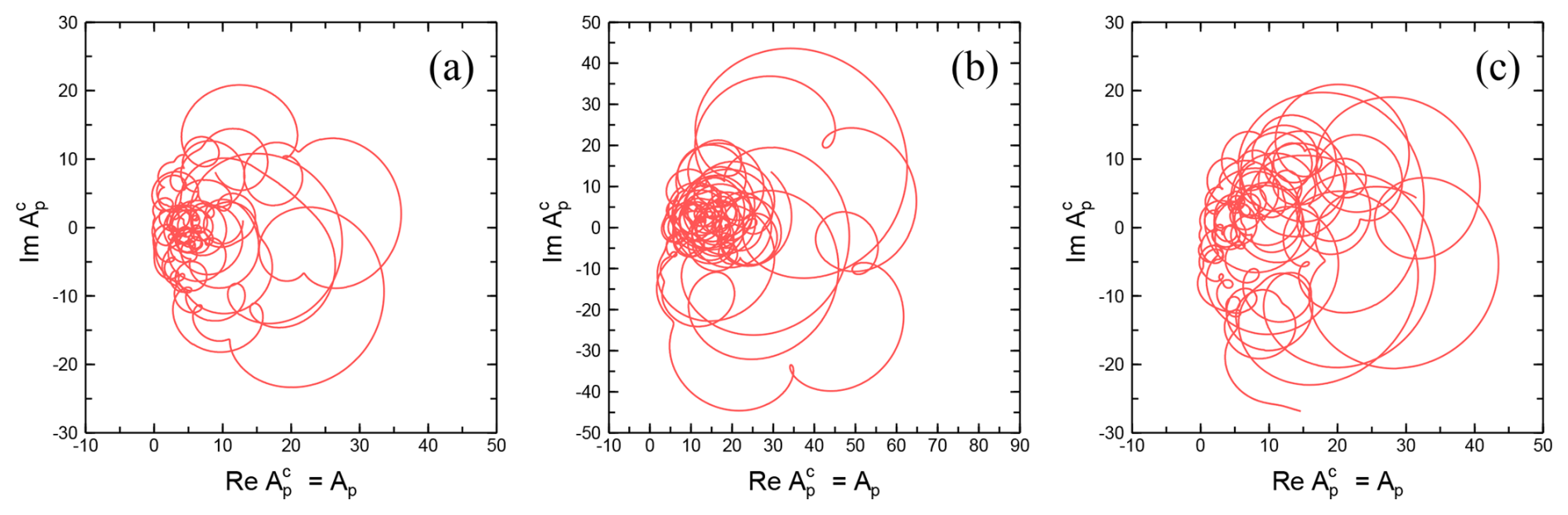
The right part of Eq. (2) suggests a complex form of Ap,

$$\begin{array}{}\text{(15)}& {\mathrm{Ap}}^c\left(t\right)=\sum _{n=\mathrm{0}}^N{c}_{nl}{\mathrm{e}}^{i\left\{n\mathit{\omega }\left[t-\left(\frac{l}{K}+\frac{\mathrm{1}}{\mathrm{2}}\right)T\right]-{\mathit{\varphi }}_{nl}\right\}}.\end{array}$$

The real part of Ap^c is equal to Ap. The hodographs (Fig. 6) show the behavior of the complex Ap^c. A hodograph represents the path traced out by the tip of a vector (here a complex number) as it moves over time. No physical conclusions are drawn from the imaginary part. The hodographs reveal clear differences in geomagnetic activity across solar cycle phases: February 2001 (solar maximum) shows large, widely spread loops indicating intense storm activity, while February 2003 exhibits more compact trajectories with moderate disturbances. By contrast, February 2017 (solar minimum) shows fewer and tighter loops, reflecting quieter geomagnetic conditions.

Our intention was to search for changes in the c_nl coefficients (or phases) with geomagnetic activity. We anticipated that the higher-frequency coefficients intensify during disturbed periods. However, we do not see any distinct behavior of the coefficients with respect to Dst in Fig. 2. Therefore, we calculate the ratio of RMSs of the Fourier coefficients c_nl within two harmonic bands, namely RMS for n = 15–20 over RMS for n = 5–10, for every selected l. The ratio (with l converted to time) is shown as brown lines in Fig. 1. Here, the dashed and dotted horizontal lines indicate 0 and 0.5 values of this RMS ratio, respectively.

Similarly to Fig. 2, we do not see any one to one correspondence between the RMS ratio and geomagnetic activity in Fig. 1. However, one event drew our attention, namely a distinct substorm during 13–14 February 2001, in panel (a). A Dst decrease is followed by a recovery, the Ap values are greater than 20 nT. The event coincides with a distinct decrease in the RMS ratio, which means a suppression of higher frequencies, which was unexpected for us, because we anticipated an opposite effect, as has been mentioned above.

4 Discussion and conclusions

Fourier analysis of the linearly interpolated Ap index is performed for three monthly periods in 2001, 2003, and 2017. The coefficients near cos nωt and sin nωt in a Fourier series have been found. The Fourier reconstruction of Ap works well. One can see that the reconstructed Ap is in good agreement with the original data. The Fourier sum usually reconstructs functions better than the Fourier transform. In addition, one can add an imaginary counterpart, and thus hodographs can be plotted. The hodograph of February 2017 is uniformly spread over the complex surface, while those of 2001 and 2003 reveal a tendency for concentrations in a region close to the origin. This could be general properties of quiet and disturbed periods.

The Fourier coefficient magnitudes and phases change smoothly with time, while the index Ap is not very smooth. Our idea was that abrupt changes in the Ap index could be predicted based on analysis of variations in Fourier coefficients before abrupt changes occur. However, the presented analysis did not support it.

We noticed that during the 13–14 February 2001 substorm, intensity of higher frequencies decreases with respect to lower frequencies, which is an unusual and unexpected effect. Whether it is a general effect, or if it only holds for some class of substorms, or it is a mere coincidence, it deserves a future analysis. If it is the case for most geomagnetic storms, then there is no solar effect on the auroral index Ap and it is mainly determined by processes intrinsic to the magnetosphere.