JUICE-MAJIS Earth observations during the 2024 gravity assist: first analysis and comparison with PRISMA data

The JUpiter ICy moons Explorer spacecraft (JUICE) performed a Lunar-Earth gravity assist maneuver on 20 August 2024, during which the scientific instruments were turned on to test their functionality. In the time of the Earth flyby, the Moon and Jupiter Imaging Spectrometer (MAJIS) on board JUICE acquired a sequence of multispectral images over the Western Pacific Ocean at tropical latitudes. In parallel, an observing campaign was also conducted by the Earth-orbiting PRISMA imaging spectrometer, with the purpose of validating MAJIS spectral observations with independent measurements of the same kind.

These two datasets are here exploited to investigate and compare several atmospheric and cloud properties, including composition, temperatures, and atmospheric gravity waves. In the MAJIS spectral range, covering the 500–5560 nm wavelengths, we identified major and minor atmospheric gases, including O₂, H₂O, CO₂, O₃, CH₄, N₂O. Since MAJIS observations mostly covered diffuse cloudiness over the ocean, our analysis mainly focused on the discrimination of clouds' features and altitudes. We verified that ice particles are widespread in the data, allowing for an investigation of their properties (e.g. crystallinity) through different spectral signatures. The only land features identified in MAJIS data are not observed in daylight, hence only a thermal emission analysis is presented. Finally, the coverage of the 4300 nm CO₂ band enables the identification of high altitude structures, revealing the presence of several atmospheric wave packets, likely induced by convective events, or lightning strikes known to have occurred at the time of the flyby. The present analysis demonstrates how MAJIS data can contribute to the scientific investigation of an atmospheric environment, and provide the first benchmark in the analysis of water ice, whose characterization in the Jovian system will be of primary importance for the JUICE mission.

1 Introduction

The JUICE mission is conceived for the investigation of Jupiter's icy satellites' surfaces and interiors, but also for the characterization of the giant planet's atmosphere and magnetosphere. These scientific objectives will be achieved thanks to a payload consisting of several remote sensing and in-situ instruments, including an altimeter, a magnetometer, a gravity experiment, a radio instrument, neutral/energetic particles and plasma detectors and an ultraviolet spectrograph. Moreover, the visible-thermal infrared spectral range will be investigated by a visible camera (JANUS) and by the Moons and Jupiter Imaging Spectrometer (MAJIS, Poulet et al., 2024b), which in particular will allow the spectroscopic investigation of Jupiter's atmosphere, moons and rings system.

On the 20 August 2024 the JUICE spacecraft performed a Lunar-Earth Gravity Assist (LEGA) and is now headed for a second Earth Gravity Assist (EGA) happening in September 2026. In this study we will focus on 2024 EGA data acquired by MAJIS which, along with JANUS (see Hueso et al., 2026), was turned on providing its very first observations of a planetary target (for a general overview of the flyby refer to Poulet et al., 2026, while valuable information about MAJIS operations, functioning and performances is given in Langevin et al. (2026) and Seignovert et al., 2026). During the flyby, different Earth observing spectrometers were coordinated to provide spatially and temporally comparable observations (Poulet et al., 2026). A companion paper by Guerlet et al. (2026) is focused on MAJIS IR channel's data comparison with co-located acquisitions by the IASI thermal Fourier spectrometer onboard the EUMETSAT/Metop satellite. Instead, we exploit PRISMA spectrometer data as a proxy to compare with MAJIS VISNIR channel observations (Sect. 2.1), even if the different times and regions of acquisition prevent a direct comparison of the scans (see Sect. 2). PRISMA (Sect. 2.2) is a technology demonstrator mission completely funded by the Italian Space Agency (ASI) and devoted to the qualification of a panchromatic/hyperspectral technology for monitoring the Earth at visual-near infrared wavelengths at moderate spectral resolution and high spatial resolution (Pignatti et al., 2013).

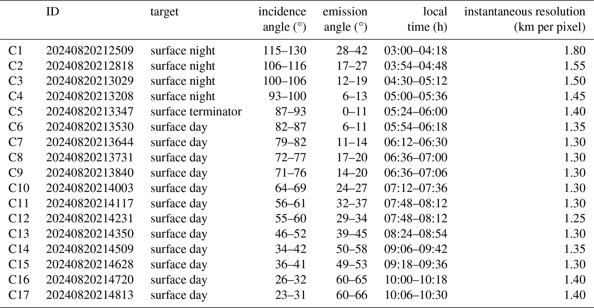
During the EGA, JUICE flew over Western Pacific Ocean at tropical latitudes, moving approximately from Sumatra to Hawaii islands and spanning local times from about 03:00 to 10:30 (see Table 1). The majority of these measurements took place over the ocean, allowing a broad characterization of atmospheric gaseous composition and structure (Sect. 2.3.2). Land features are only marginally detected in a couple of observations mainly in the thermal range (Sect. 4.4).

Given the widespread presence of clouds and the early local times of acquisition (Sect. 2), ice is observed in almost all MAJIS scans (Sect. 4.1), allowing benchmarking of the spectrometer's response to this observable in view of Jupiter's icy satellites investigation. Also atmospheric waves (whose role is fundamental in regulating the middle-atmosphere circulation, e.g. Hamilton, 1996; Fritts and Alexander, 2003) are detected in many MAJIS observations. Such phenomena are either linked with orography (Queney 1948; Kim et al. 2003) or with the occurrence of thunderstorms (Taylor and Hapgood, 1988; Dewan et al., 1998). Given that MAJIS EGA observations mainly targeted the ocean, we investigate the waves' connection with strong convective events or lightning strikes (Sect. 4.4).

The manuscript is arranged in sections describing the data (Sect. 2), the methods for their investigation (Sect. 3) and the obtained results (Sect. 4). Such a wide ensemble of atmospheric observable features is finally discussed in the context of Jupiter science in Sect. 5.

2 Observations

2.1 MAJIS EGA Data

MAJIS is a dispersion grating imaging spectrometer operating between 500 and 5560 nm by means of two spectral channels (Poulet et al., 2024b). The first channel (VISNIR, 500–2350 nm) is characterized by nominal spectral resolution and sampling of 2.9–4.6 and 3.5–3.8 nm per band respectively, while the second (IR, 2270–5560 nm) works with a spectral resolution of 5.5–7.0 nm and a sampling of 5.9–6.9 nm per band. The nominal instrument's instantaneous field of view (IFOV) is 150 µrad per pixel. MAJIS concept has been optimized for the characterization of the surface and near-surface environment of Jupiter's icy moons (Poulet et al., 2024b), as well as for the investigation of Jupiter's atmosphere (Fletcher et al., 2023). Detailed descriptions of the instrument functioning, operations and calibration are given in Haffoud et al. (2024), Langevin et al. (2024), Poulet et al. (2024a), Filacchione et al. (2024), Rodriguez et al. (2024), Vincendon et al. (2024), and Stefani et al. (2025). Scene geometry is reconstructed via the SPICE-NAIF toolkit (Acton, 1996; Acton et al., 2018) and kernels provided by ESA (ESA SPICE Service, 2019).

Figure 1 and Table 1 summarize footprint locations and main basic properties of the 17 MAJIS EGA data investigated in this work (see Poulet et al., 2026, for further instrumental parameters). Two additional cubes, targeted off-limb for calibration purposes (Poulet et al., 2026), are not considered here. Each MAJIS acquisition consists of hyperspectral cubes (i.e. 2D spatial frames with a third spectral dimension) collected as pushbroom spectral scans via internal mirror rotation, with different widths and lengths.

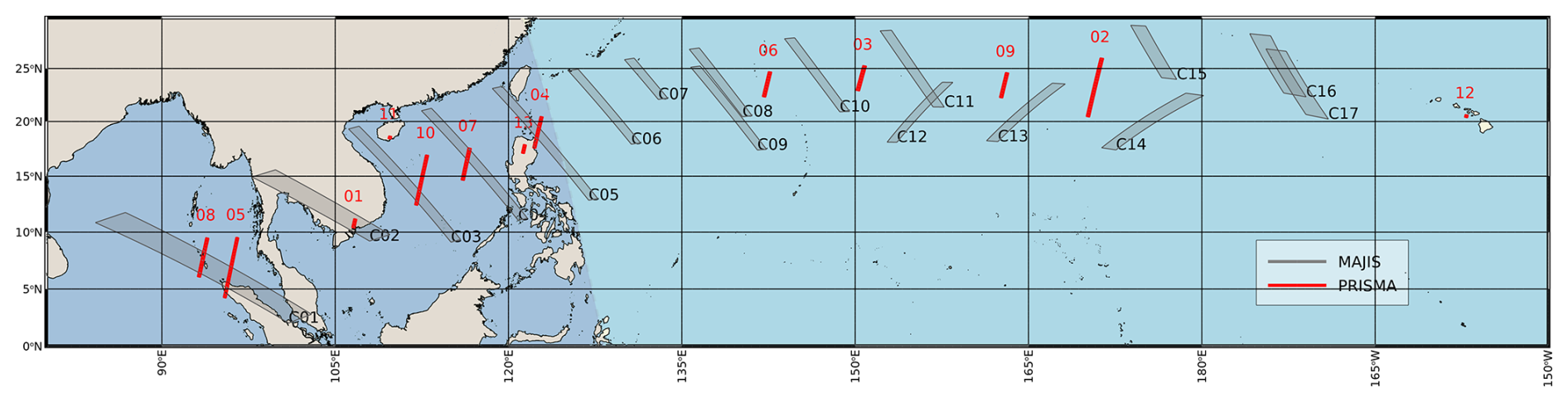
Figure 1 Geographical coverage of the investigated observations, MAJIS in grey color, PRISMA in red color. The darker area westward of the Philippines indicates the nightside at the time of the terminator crossing of MAJIS observations (20 August 2024, 21:30 UTC). Instead all PRISMA footprints are in daylight, at local time ∼10:30. Coastlines are from OpenStreetMap, available under the Open Database License.

The first 4 cubes (C1 to C4) pointed to the Earth surface at nighttime and contain a significant signal only in the thermal part of the spectrum (λ>3000 nm). The only exception is C1, where a lightning emission is identifiable at visible wavelengths (D'Aversa et al., 2026). C5 is straddling the terminator and is the first cube containing information on the dayside ocean and clouds. Some coastlines are identifiable in C4 and C5 at thermal wavelengths, as it will be discussed in Sect. 4.4. All the subsequent cubes (C6 to C17) are acquired in daylight and hence the full spectrum can be investigated, even if they only cover the ocean mostly under cloudy/stormy conditions.

Cubes C11, C12 and C13 have been acquired with longer integration times, with the purpose of testing the instrument response. This leads to signal saturation in many regions (especially at visual wavelengths over clouds, see Sect. 2.3.1), that have been removed from our analysis. The spatial resolution in this dataset is quite stable (about 1.4 km per pixel, slightly affected by motion smearing) and is suited for the investigation of both homogeneous and localized cloud structures. On the other hand, the IFOV is affected by unresolved cloudiness (likely widespread) which dilutes the low reflectivity of deep water hence preventing the acquisition of clear-sky ocean (Sect. 2.3.1, Fig. 2).

Table 1 MAJIS observing parameters during EGA. Phase angle is always close to 90°.

2.2 PRISMA data

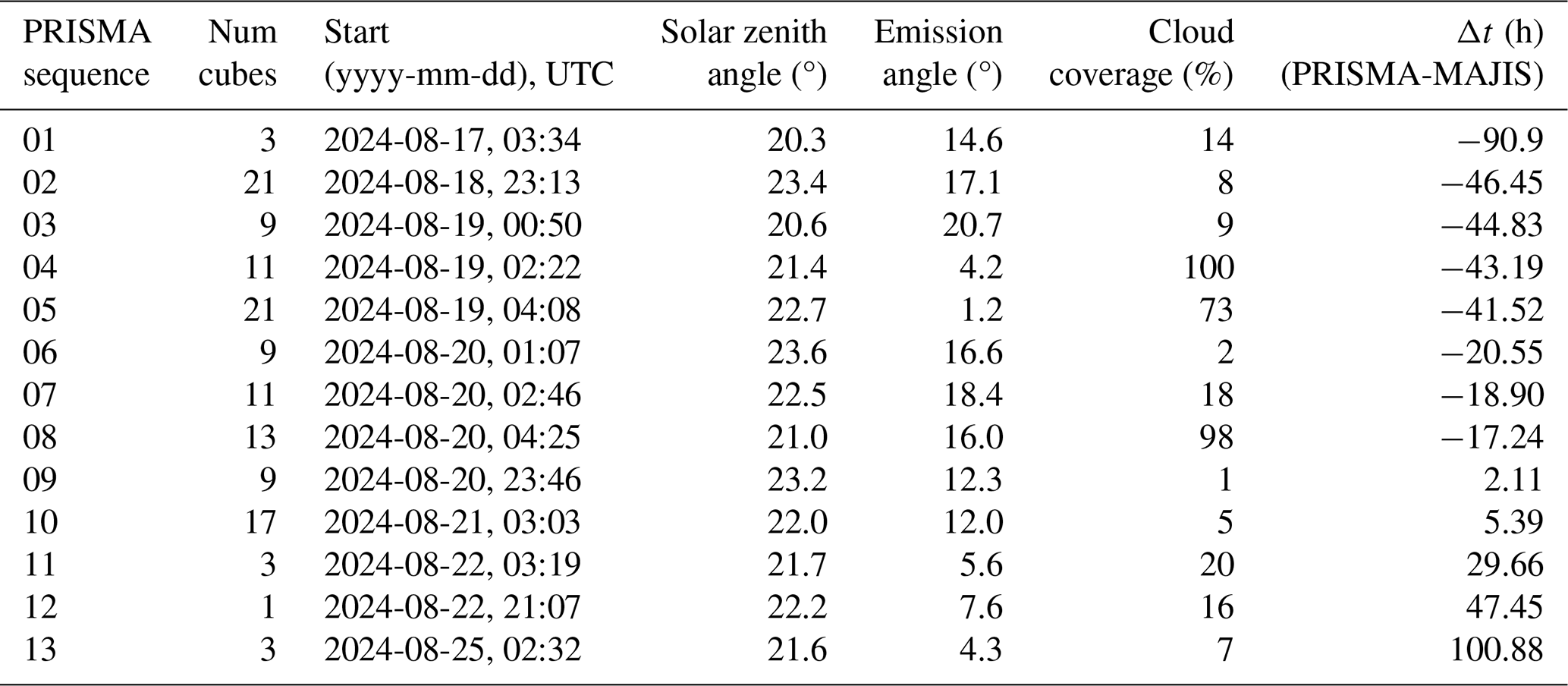
An observing campaign coordinated to the EGA was conducted by the mission PRISMA (PRecursore IperSpettrale della Missione Applicativa), managed by the Italian Space Agency. The mission hosts a visible and near-infrared imaging spectrometer, covering a range (400–2500 nm) compatible with the MAJIS-VISNIR channel but having a coarser spectral resolution (∼12 nm) in turn compensated by a higher spatial resolution (∼30 m per pixel). Details about the instrument and the mission can be found in Pignatti et al. (2013), while mission characteristics, access, products, calibration, geometry navigation and data policy are fully described in Lopinto et al. (2021).

PRISMA sequences (13 in total, red rectangles in Fig. 1, main parameters summarized in Table 2) consist of a variable number of 30 km × 30 km hyperspectral cubes, each composed of 1000×1000 spatial pixels. Due to the PRISMA orbit (Sun-Synchronous-Low-Earth-Orbit), observations are acquired at a fixed solar local time (∼10:30), making it impossible to achieve spatial/temporal coincidence with MAJIS ones (see next section).

Table 2 PRISMA observations acquired in coordination with JUICE.

2.3 General comparison overview

Both MAJIS and PRISMA acquired multispectral data covering the same kinds of structures, offering a useful benchmark for checking MAJIS capabilities in detecting and analyzing specific features of scientific interest. In the following section we investigate how the spectral signatures of the main atmospheric gases and of clouds are affected by the different spatial/spectral resolutions and observing conditions. When reflectances are discussed, they are obtained for both instruments as $I/F$, where I is the observed spectral radiance and F is Kurucz solar spectral radiance (Kurucz et al., 1984; Kurucz, 1995) available at the website https://earth.gsfc.nasa.gov/climate/projects/solar-irradiance/data (last access: 10 February 2026). For readability, in the following we will refer to spectral radiance simply as radiance.

2.3.1 Ocean/clouds spectra first comparison

Figure 2 shows the two PRISMA and MAJIS cubes that are closest from both a spatial and temporal point of view (∼550 km and ∼2 h apart), covering open ocean areas overlaid by a different amount of clouds. In this framework, the most robust radiance comparison should consider ocean cloud-free spectra, expected to be quite stable in space and time and very dark at visual wavelengths (given the very low ocean albedo, ∼4 %). However, the comparison between the two instruments (Fig. 2E) highlights that the darkest MAJIS signals are still brighter than those from PRISMA, possibly suggesting enhanced cloud/aerosol content. Indeed, the higher spatial resolution of PRISMA data reveals a number of small-scale structures, likely unresolved by MAJIS, yet affecting its signal. For instance, the small bright feature imaged by PRISMA in Fig. 2D, covering only a portion of a MAJIS pixel footprint, may induce spectral variations of the ocean spectrum up to 50 % (Fig. 2F) once observed at the MAJIS resolution scale.

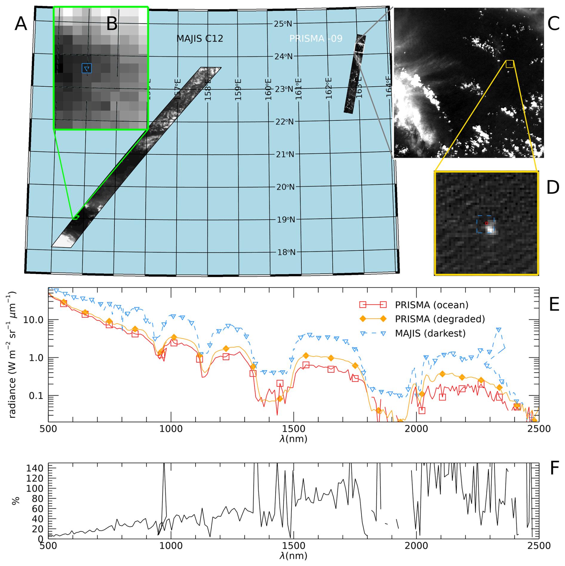
Figure 2 (A) MAJIS observation C12 and PRISMA sequence P09 (∼2 h apart) shown at 875 nm in an equal-area projection. (B) Blow-up of the darkest area in the MAJIS image, highlighting individual pixels' size (the pixel with the lowest signal is highlighted in blue). (C) The second cube of the PRISMA sequence is shown in its full extension of 1000×1000 pixels. (D) Blow-up of an area of PRISMA data encompassing a small bright cloud. The blue dashed box shows the approximate size of a MAJIS pixel. (E) Single-pixel spectra from the darkest pixels of MAJIS (blue color, triangle symbol in (B) and PRISMA (red curve, red square in D). The orange curve represents a PRISMA spectrum degraded to MAJIS spatial resolution (average inside the blue box of panel D). The MAJIS spectrum is multiplied by the ratio of solar incidence cosines (=1.82) to achieve a radiance level comparable with PRISMA. (F) Spectral effect of the spatial degradation in PRISMA data, shown as the relative difference between the red and orange curves of panel (E).

Most of the spectral variability in both datasets is driven by changes in the H₂O absorption bands. Besides the general low reflectivity, ocean spectra are characterized by the presence of large and often saturated water absorption bands. On the other hand, H₂O clouds (either composed of liquid droplets, ice crystals or a mixture) can easily be identified through RGB imaging from both datasets due to their bright appearance (Sect. 3.1). H₂O bands are less saturated over clouds, where light scattering prevents photons from reaching the underneath, more absorbing, atmospheric layers. Ice clouds' discrimination is basically driven by the spectral shift of absorption bands between solid and liquid H₂O phase (Sect. 3.1). The comparison of spectral signatures related to the ocean and clouds (main spectral endmembers for both instruments) is shown in Fig. 3A–B in log and linear scale respectively (refer to Figs. 4 and 5 for the gaseous features identification). This comparison should be considered as qualitative, since spectra acquired at different locations, geometries and local times are being considered (see Tables 1 and 2). Therefore, clouds are likely characterized by different vertical distributions and microphysical properties, driven by a radiative forcing that is changing between early and mid-morning. Also, differential sun-glint effects (dependent on geometry and wind strength) could produce differences in the overall reflectivity of the ocean (Cox and Munk, 1954). All these effects (straylight could also have an impact here, see Langevin et al., 2026) are likely to contribute to non-linear offsets in the continuum below about 700 nm (e.g. Zinner et al., 2016), and slightly different depth and shape of water absorption bands, not ascribable solely to differences in spectral resolution.

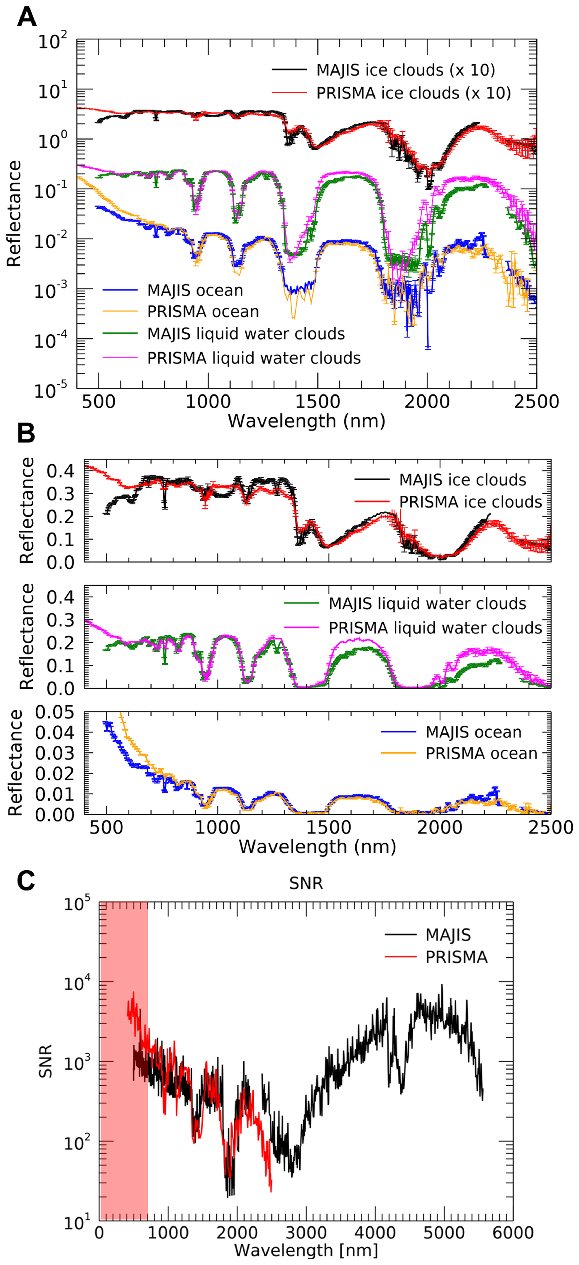
Figure 3 Comparison between MAJIS and PRISMA reflectances in log (A) and linear (B) scales related to ocean, liquid water clouds and ice water clouds (the latter multiplied by 10 for clarity in panel A). PRISMA spectra are selected from two orbits in session 7, MAJIS ones from orbits C7 (ice clouds) and C10 (ocean and liquid water clouds). Panel (C) shows the SNR estimated for the two instruments (cube C15 for MAJIS, one cube of session 07 for PRISMA) as described in Sect. 2.3.1. The red shaded area indicates the spectral region possibly affected by straylight contamination, not yet fully assessed in both datasets.

The three endmembers in Fig. 3 show similar trends in reflectivity, with the main absorption bands' shape correctly reproduced, even if the probed atmospheric structure is probably not the same. For example, MAJIS liquid water clouds spectrum shows wider wings and a flatter bottom for the bands at 1400 and 1900 nm, suggesting different scattering properties in the atmospheric column for the two cases (see Sect. 4.2.4). A slightly flatter bands' bottom is also observed in the ocean spectrum (blue compared to the orange PRISMA spectrum). On one side, this could indicate that early-morning thin clouds in the mid-high troposphere are mixed in MAJIS footprint, preventing the formation of the narrower water lines inside the bands (MAJIS spectrum refers to 07:30 local time, when the presence of unresolved hazes is likely). On the other hand, such low signals could reach the instrument noise equivalent spectral radiance (NESR), hence explaining the featureless bands' bottom. We derived an upper limit for the NESR by investigating the darkest ocean region in the selected MAJIS cube (C10), resulting in about 10⁻³ $\mathrm{W}{\mathrm{m}}^{-\mathrm{2}}\mathrm{\mu }{\mathrm{m}}^{-\mathrm{1}}{\mathrm{sr}}^{-\mathrm{1}}$ at 1900 nm. This value corresponds to reflectances of 10⁻⁴, about one order of magnitude below the ocean signal at that wavelength (Fig. 3A), hence making the mixed-footprint hypothesis more likely. The occurrence of saturation in some parts of MAJIS spectrum is highlighted in the ice clouds comparison, evident as a broad absorption between 900 and 1100 nm in Fig. 3B. MAJIS uncertainties are extensively discussed in the paper by Poulet et al. (2026), but here we attempt an a posteriori estimation of the spectral signal to noise ratios (SNR) for both instruments by performing a statistical analysis of spatial fluctuations computed in 5×5 pixels boxes (Fig. 3C). For each wavelength (excluding saturated regions) we select those regions producing the minimum relative error, hence representing both noise statistics and true variations in the observed scene. As a result, the spectral SNRs in Fig. 3C refer to wavelength-dependent locations in the respective cubes, rather than to a single region. This means that the high frequency oscillations in the red and black lines are mostly driven by spatial differences between the selected boxes (at the scale covered by the respective cubes). Values below ∼700 nm (red shaded area in Fig. 3C) could be driven by differences in clouds/aerosols' properties (in turn impacting the intensity of Rayleigh scattering), and are possibly contaminated by the presence of straylight affecting the actual trend of the SNR for both instruments.

2.3.2 Gaseous compounds

Figure 4 compares sample MAJIS/PRISMA liquid water clouds reflectance spectra with two-way vertical transmission due to O₂, H₂O, CO₂, CH₄, N₂O and O₃, based on an average vertical structure from Efremenko and Kokhanovsky (2021) and calculated through the line-by-line method with line parameters from the HITRAN database (Gordon et al., 2022) and from O₃ cross sections by Gorshelev et al. (2014) and Serdyuchenko et al. (2014). Finally, transmissions are convolved at the MAJIS spectral resolution.

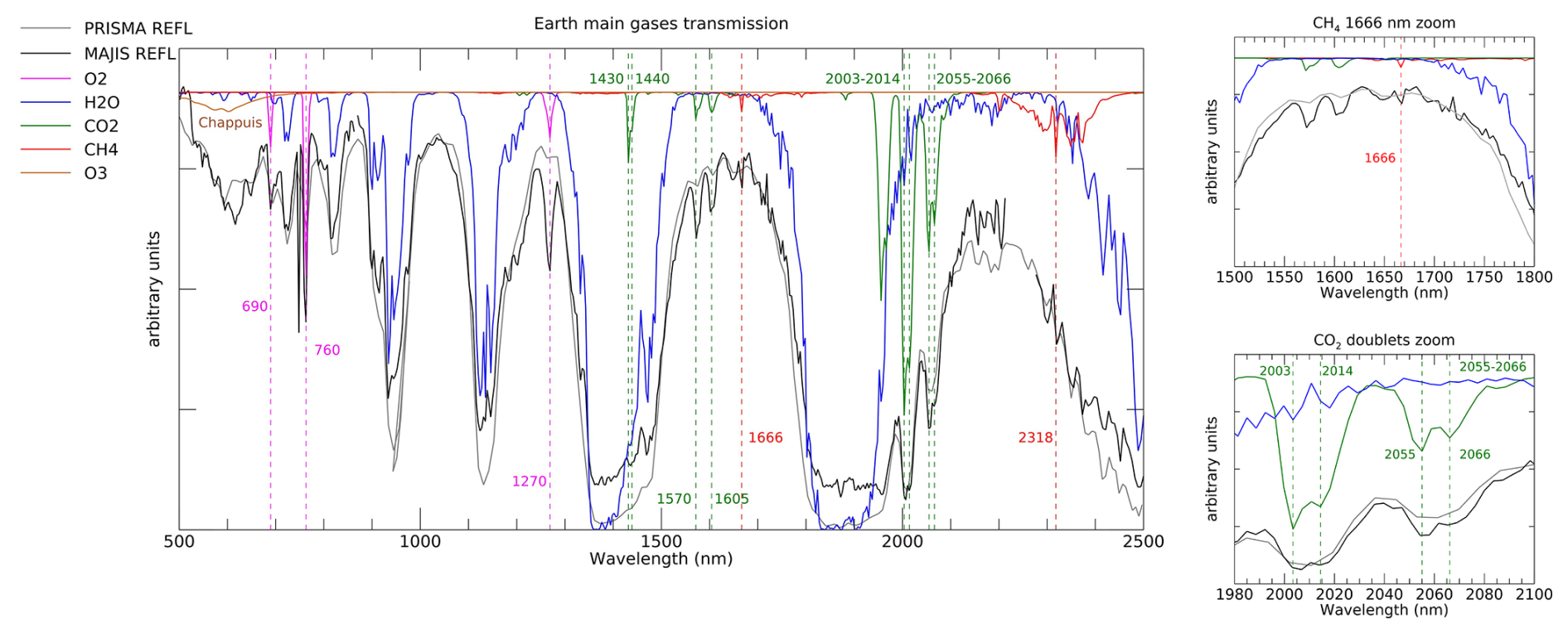
Figure 4 MAJIS (black, taken from C7) and PRISMA (grey, taken from session 7) normalized reflectances (both pertaining to liquid water cloud scenarios) compared to main Earth's atmospheric gases two-way transmissions convolved on MAJIS spectral grid. Vertical dashed lines indicate the main non-H₂O molecular lines identifiable in the observations. Zooms related to the CH₄ 1666 nm absorption line, and the CO₂ doublets at 2003–2014/2055–2066 nm are shown in the upper and lower right panels respectively.

In their common spectral range, both instruments allow to identify the main absorption features of H₂O, O₂ and CO₂ (Fig. 4, see also Poulet et al., 2026). The reduced spectral resolution of PRISMA makes it difficult to resolve narrow features like the methane absorption at 1666 nm (Fig. 4, upper right panel), the close doublets of CO₂ at 2003–2014 nm and 2055-2066 nm (Fig. 4, lower right panel), or shallower lines of water. On the other hand, the PRISMA spatial resolution is expected to reduce the spatial mixing of different types of surfaces or aerosols, allowing a more robust tracking of localized and transient phenomena (e.g. smog layers, ice patches, oil spills, CO₂ emissions, etc.). At wavelengths around 600 nm a broad absorption possibly matching the O₃ Chappuis band appears in both datasets. In MAJIS, this is enhanced over thick clouds and in particular in grazing illumination conditions (Sect. 4.4) in which the atmospheric column above ∼20 km is directly illuminated resulting in a very long photon path length that increases the absorption from O₃ in the scattered light (most of terrestrial ozone resides between altitudes of 20 and 40 km). Nevertheless, a better quantification of this feature requires a more rigorous assessment of the straylight contamination (Langevin et al., 2026).

Besides the better spectral resolution, MAJIS also has the advantage of an extended spectral range covering wavelengths from 2500 up to 5560 nm. In this range, thermal emission dominates and provides information on the temperature of the sampled atmospheric layers, or of the ocean and clouds. This interval is characterized by several H₂O absorption bands (the stronger one centered at about 2700 nm), strong and saturated CO₂ ones at 2690, 2770 and 4300 nm, and weaker CH₄, O₃, CO and N₂O signatures (Fig. 5, see also Guerlet et al., 2026). In particular, the strong CO₂ absorption (and emission) at 4300 nm, can be used for the estimation of the vertical structure of atmospheric temperatures (see Poulet et al., 2026).

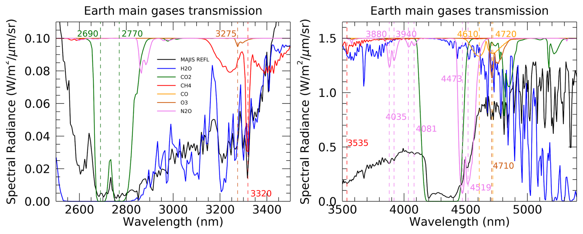
Figure 5 MAJIS (black) spectral radiance compared to main Earth's atmospheric gases two-way spectral transmissions (offset for clarity) in the 2500–3500 nm range (left) and 3500–5400 nm range (right). Thermal emission is not considered in the transmission computation and all spectra are convolved to the MAJIS spectral grid.

3 Methods

In this section we describe different methods for investigating the information content in the data, including surface/cloud features identification (Sect. 3.1), ice characterization (Sect. 3.2), clouds' altitude estimation (Sect. 3.3) and high-altitude features investigation (Sect. 3.4).

3.1 Surface and clouds identification

In principle, Earth observations can encompass different types of surfaces, commonly discriminated spectrally through indices expressed in the formalism of Normalized Difference spectral Indices (NDIs, see Wolf, 2012, for a general review). Useful examples are given in Hurley et al. (2014) (dealing with Rosetta/VIRTIS-M data, Coradini et al., 1999) and in Oliva et al. (2017) (dealing with both Rosetta and Venus Express/VIRTIS-M data, Drossart et al., 2004). Table 3 summarizes these indices (derived from spectral endmembers from Rosetta/VIRTIS-M acquisitions, Fig. 6A–B, since MAJIS observations did not cover surface features in daylight) that we test on PRISMA data (Fig. 6C–D) as a benchmark for the future September 2026 EGA, in which Africa observations are planned. A new ocean index is also defined specifically for MAJIS data, which do not cover all wavelengths of the nominal ocean NDI. It is worth stressing that the ocean class should not be considered as representative of clear-sky conditions as it may actually include some amount of aerosol opacity (Sect. 2.3.1). No specific index has been adopted for generic clouds identification, but we rather assign to this class all pixels that do not meet any of the surface classes' conditions. Indices thresholds can be studied taking advantage of proxy images (e.g. the PRISMA one shown in Fig. 6C, not pertaining to EGA sequence) in which the changing reflecting structures can be clearly identified. The derived values depend on instrument features and require specific tuning when switching between different datasets. Figure 6C–D shows how the different types of spectral classes can be reliably identified, even if, in this case, no ice clouds are present. Other examples of application of the ocean, clouds and ice indices from Table 3 to MAJIS and PRISMA data are discussed in Sect. 4.1. Instead, the application of surface-related indices to MAJIS data did not result in positive identification, since land features in MAJIS data are not seen in daylight illumination, making NDIs not applicable.

Table 3 Spectral indices for the identification of different spectral classes related to surfaces and clouds. R indicates $I/F$ and the subscript is the wavelength in nanometers. A MAJIS specific condition for ocean detection is highlighted in italic (see Sect. 3.1).

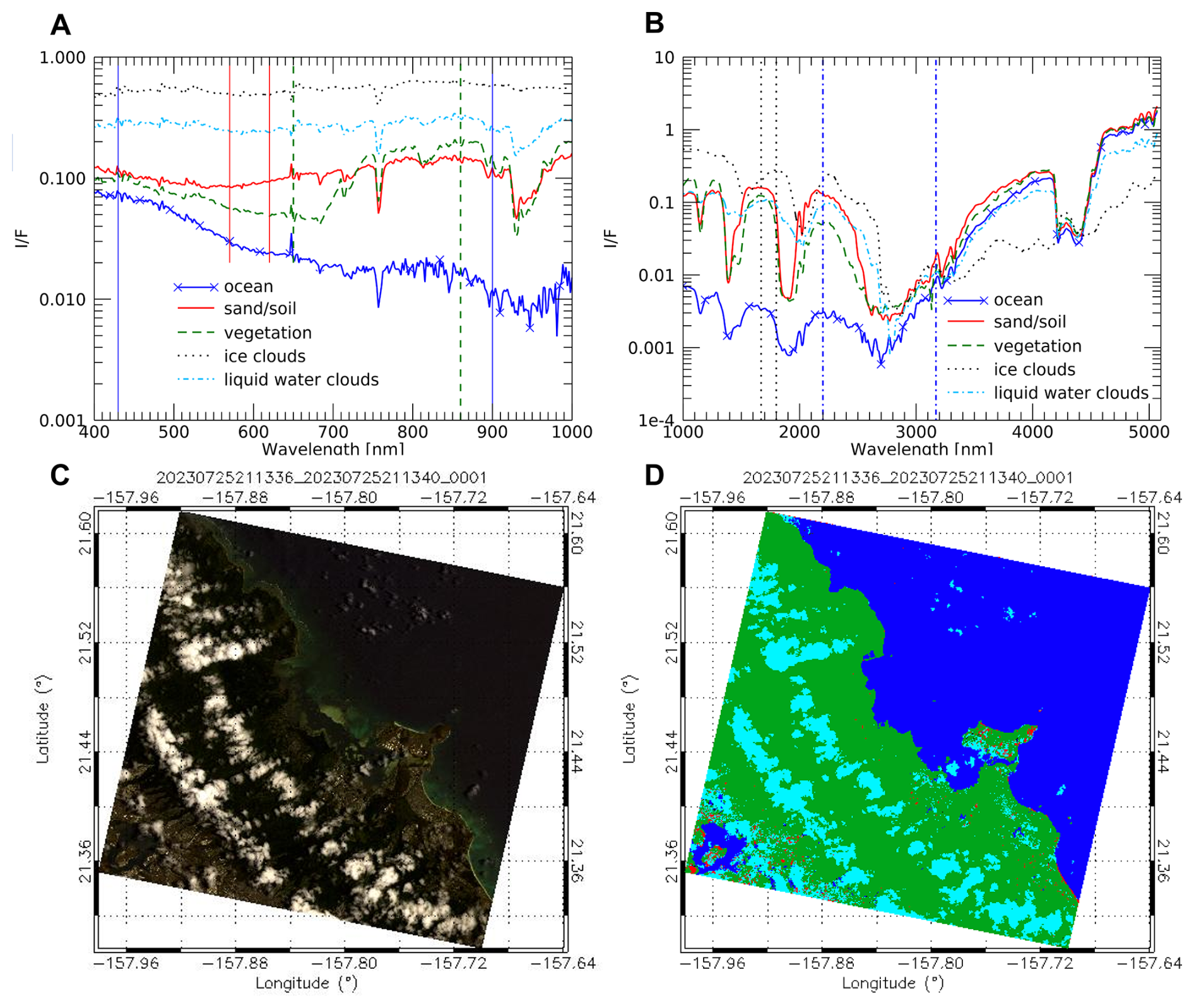
Figure 6 (A) Reflectance endmembers of different classes of surface and clouds, derived from Rosetta/VIRTIS-M VIS channel Earth observations (Oliva et al., 2017). Vertical lines share the style and color of the corresponding spectral endmember and identify the wavelengths adopted in the index definition (blue ones refer to the NDWI). (B) same as in (A) but $I/F$ spectra from the NIR channel of VIRTIS-M are shown (vertical blue dashed-dotted lines refer to the MAJIS ocean index). (C) Example of a PRISMA RGB image covering different surface types (data cube 2023072521336_20230725213340) targeting the eastern coastal line of Honolulu island (R=680 nm; G=570 nm, B=440 nm). (D) distribution of spectral classes obtained from the spectral indices in Table 3. Green pixels indicate vegetation, red ones are sand, cyan ones are clouds, blue ones indicate ocean/water (no ice clouds present).

In the specific conditions of MAJIS EGA sequence, the most robust land identification must rely on soil/ocean contrast in thermal emission (Sect. 4.4), triggered by the different thermal inertia of the two classes. However, also the presence of clouds in the line of sight induces a decrease of the observed brightness temperature (T_B), hence land identification requires matching the shapes of low T_B regions within known coastlines. The largest land region emerging in this way is shown in Fig. 7 (cube C4), (Philippines's Busuanga and Coron islands in cube C4), whose identification also allows a refinement of MAJIS pointing reconstruction (Seignovert et al., 2026). The largest brightness temperature contrast for both land/ocean and cloud/ocean cases occurs in the 3500–4000 and 4600–4800 nm spectral ranges, which are less absorbed by atmospheric H₂O and CO₂. The application of this method to other MAJIS data is illustrated in more detail in Sect. 4.4.

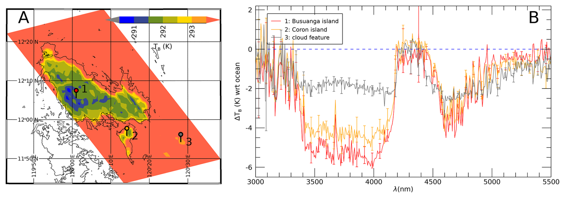
Figure 7 Land detection obtained by comparing the shapes of low brightness temperature (T_B) regions in MAJIS cube C4 with known coastlines. (A) Identification of Busuanga and Coron islands (markers 1 and 2 respectively), colder than the surrounding ocean, as well as clouds (marker 3). (B) Spectral contrast in brightness temperature (T_B) with respect to the ocean spectrum, measured over the islands (Busuanga in red, Coron in orange) and over a thin cloud (grey curve). Coastlines data from OpenStreetMap, available under the Open Database License.

3.2 Ice characterization

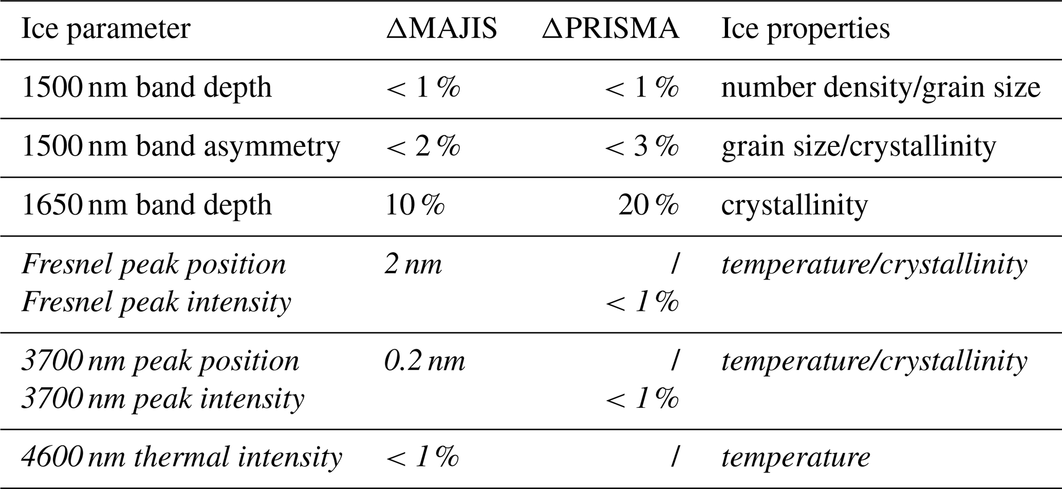
MAJIS and PRISMA data allow investigating the distribution of physical properties of ice and how they relate, for example, to the altitude of the clouds where it is identified (see Sect. 4.1 and 4.2). The temperature, crystallinity, grain size, purity, and density affect the shape of ice absorption bands (in particular the main ones at 1500 and 1900 nm) and of the continuum. Since the long wavelength shoulder of the 1900 nm band encompasses the noisy junction between the VISNIR and IR channels of MAJIS, we focus on the 1500 nm band, spectrally well resolved in both MAJIS and PRISMA datasets. This band has a characteristic asymmetry (due to its differential intensity with respect to the 1900 nm one, e.g. Stephan et al., 2021a) affecting the position and shape of the in-between transmission window peak (∼1700 nm) and has been used for the definition of the ice index in Table 3. Within the 1500 nm band, the weaker 1650 nm absorption is present. Its strength is a proxy for the degree of the ice crystallinity and temperature (Fink and Larson, 1975; Filacchione et al., 2016). It is also observable in PRISMA, even if shallower and noisier due to the lower spectral resolution (see zooms in Fig. 8A and B).

The 3000–4000 nm wavelength range, not accessible to PRISMA, hosts two ice reflection peaks at around 3100 nm (the Fresnel peak) and 3700 nm (Fig. 8C). The former varies in shape and intensity as a function of the ice crystallinity (Cartwright et al., 2025) while the latter shifts to longer wavelengths as temperature increases (e.g. Filacchione et al., 2016, see Sect. 3.3.3). Fresnel peak position variations are estimated in the data through cross-correlating each ice spectrum with a constant shape (average peak shape in each cube) which is rigidly shifted with a 0.1 nm sampling (hence allowing the estimation of the peak with a sampling better than the nominal MAJIS one). On the other hand, the 3700 nm peak position is obtained through fitting with a Gaussian function, reliably reproducing its shape.

Another proxy of the ice temperature is the intensity of its thermal emission, becoming significant at wavelengths larger than 4500 nm (Fig. 8D). However, in this range the emitted radiance is absorbed by a plethora of narrow bands of gaseous water, and therefore only a narrow transmission window around 4600 nm is suitable for this purpose. Table 4 summarizes these ice spectral features, identifiable in MAJIS and PRISMA data. The average uncertainties Δ are propagated taking into account the SNR estimates described in Sect. 2.3.1.

Table 4 Investigated ice spectral parameters and related average uncertainties (Δ) and ice properties. Entries in italics indicate parameters that only refer to MAJIS dataset.

As a first investigation of the ice spectral variability in MAJIS and PRISMA observations we take advantage of the unsupervised K-means classification algorithm included in the ENVI software package, version 6.0 (Exelis Visual Information Solutions, Boulder, CO, USA, https://www.nv5geospatialsoftware.com/Products/ENVI, last access: 15 December 2025). This algorithm is capable of grouping the observations into an ensemble of “K” non-overlapping clusters, driven by spectral similarity, whose average spectra are representative of the main signatures in the dataset. This is done through an iterative minimum distance technique whose details are described in Tou and Gonzalez (1974). In this preliminary analysis, we arbitrarily set the algorithm to produce K=5 output average spectra, enough for visualizing the variability of the main ice diagnostic spectral features. It must be noted that, since we are also interested in features pertaining to infrared wavelengths, in MAJIS case the full VISNIR + IR spectral range is considered, and wavelengths longward of 2500 nm contribute to the clustering as well. As we will see in Sect. 4.1, this also has an impact on the spatial distribution of the clusters. The resulting average spectra in the solar range are shown in Fig. 8A and B for MAJIS cube C16 and for one of PRISMA session 04 cubes respectively. These spectra result to be mainly driven by the changing intensity of the continuum, in turn providing information about the opacity of the ice clouds. The color scale is associated with increasing reflectance of the transmission window at 1700 nm (dashed grey, dashed red, orange, blue and green with crosses from low to high, indicating increasing opacity and variable crystal sizes). The same color scheme is retained for the intensity of Fresnel peak at 3100 nm in MAJIS data (Fig. 8C), diagnostic of the ice crystallinity. Instead, spectra with intermediate reflectances at 1700 nm switch order within the 3700 nm ice reflectivity peak (dashed red to blue to orange from low to high, Fig. 8C) indicating the increased weight of thermal emission on the overall signal in this range. At MAJIS wavelengths larger than 4500 nm (Fig. 8D) the initial color scheme is totally disrupted, due to the mixing of information about cloud emissivity, cloud temperature (i.e. the altitude) and gaseous opacity. The combination of high NIR reflectances and low thermal emission (green spectrum with crosses) suggests the presence of optically thick high-altitude clouds, as confirmed by the shallower water absorption bands longward of 4900 nm. On the other hand, large thermal radiance and deep water bands associated with intermediate NIR reflectance (dashed red spectrum) indicate a population of moderate opacity clouds at quite low altitudes. The other spectra present intermediate properties in the thermal range, not strongly correlated with the NIR reflectance, calling for mixed-phase clouds of variable microphysical properties and vertical structure.

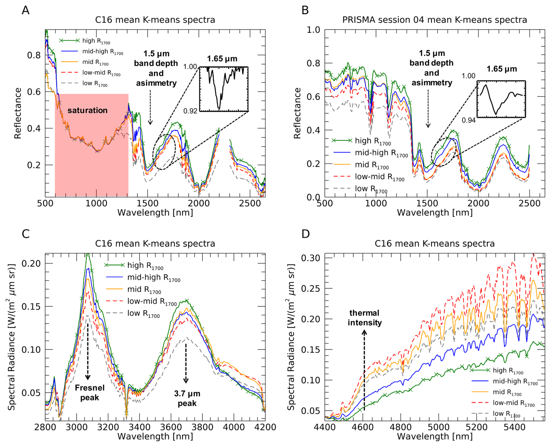
Figure 8 (A) mean reflectance spectra from the K-means clustering algorithm for MAJIS cube C16 (λ<2500 nm). The red shaded area indicates wavelengths that are saturated due to the high reflectivity of clouds. Colors indicate different regimes of the continuum reflectance, taken as reference at the 1700 nm transmission window (R₁₇₀₀). (B) same as in (A) but for PRISMA session 04 (full spectral range). The insets in (A) and (B) zoom between 1570 and 1780 nm to show the average 1650 nm band normalized to the continuum. (C) MAJIS radiances in the $\mathrm{2800}<\mathit{\lambda }<\mathrm{4200}$ nm range, zooming on the Fresnel and 3700 nm ice reflectivity peaks. (D) thermal part of the spectrum longward of 4400 nm. In all panels, dashed arrows highlight diagnostic spectral features of the ice.

3.3 Estimation of clouds' altitude

The most straightforward method for evaluating cloud altitudes involves the correlation of the brightness temperature at a given wavelength (e.g. 4610 nm, less affected by gaseous absorption in the MAJIS range) with a known vertical temperature profile. For ice clouds, temperatures can be derived from the 3700 nm peak position (Sect. 3.3.3). Other methods that we consider here are based on O₂ absorption bands' variability and on the analysis of clouds' shadows (Sect. 3.3.1 and 3.3.2). In this study, we rely on a fixed average temperature profile (Efremenko and Kokhanovsky, 2021), which may be not representative of the actual thermodynamic conditions of the atmosphere during the observations. As a consequence, all the methods that we adopt yield a range of results, each affected by their own intrinsic limitations. Although they appear quite consistent with each other, more quantitative investigations are postponed to future analyses.

3.3.1 O₂ band depth variability

The O₂ spectral features covered by both MAJIS and PRISMA observations consist of the absorption bands at 630, 690, 760 and 1270 nm (Newnham and Ballard, 1998; Smith and Newnham, 1999). As we can see in Fig. 9A, MAJIS can resolve all bands except the 630 nm one, while PRISMA data can only partially resolve the 760 nm one. The strongest 760 nm band is the most used from satellite measurements in the near-infrared (e.g. GOSAT, Butz et al., 2011; SCIAMACHY, Bovensmann et al., 1999; TROPOMI, Veefkind et al., 2012; OCO-2/3, Eldering et al., 2019) for inferring bulk atmospheric quantities like temperature profile, airmass (Stevens et al., 2017), aerosol and clouds properties (Geddes and Bösch, 2015). O₂ is a well-mixed component of the atmosphere, hence the curves of growth of its absorption bands with altitude in the presence of optically thick clouds can be translated into the altitude of the cloud top (e.g. Wei et al., 2024).

In our analysis we applied a simplified scheme for retrieving cloud top altitudes from the 760 nm band in the PRISMA case and from both 760 and 1270 nm O₂ bands for MAJIS data. The different strength of the two bands implies a different curve of growth with altitude (Fig. 9B), with the 1270 nm one less sensitive to higher clouds but more suitable for characterizing lower structures. The 630 and 690 nm bands, intrinsically weaker and more sensitive toward the surface, are not used in this analysis.

The comparison of a measured O₂ band depth with its theoretical curve of growth, evaluated for the actual airmass, allows us to directly retrieve the cloud top altitude (Sect. 4.2.1). It is worth stressing that although altitude, pressure and temperature of the cloud top are important atmospheric parameters (Nakajima et al., 2019), our simplified scheme neglects details of vertical distributions and scattering properties, introducing possible biases in the retrieved absolute values. Propagating the MAJIS uncertainties previously discussed (Sect. 2.3.1) and assuming suitable model ones (∼10 % on the oxygen vertical profile induced by local changes in gaseous temperature, density, humidity), errors on cloud top altitude average to values of ∼1 km, for both the 760 and 1270 nm bands. In addition, the 1270 nm band is known to contain a significant airglow emission feature that can alter the band depth and introduce further biases in the oxygen absorption evaluation (Kuang et al., 2002).

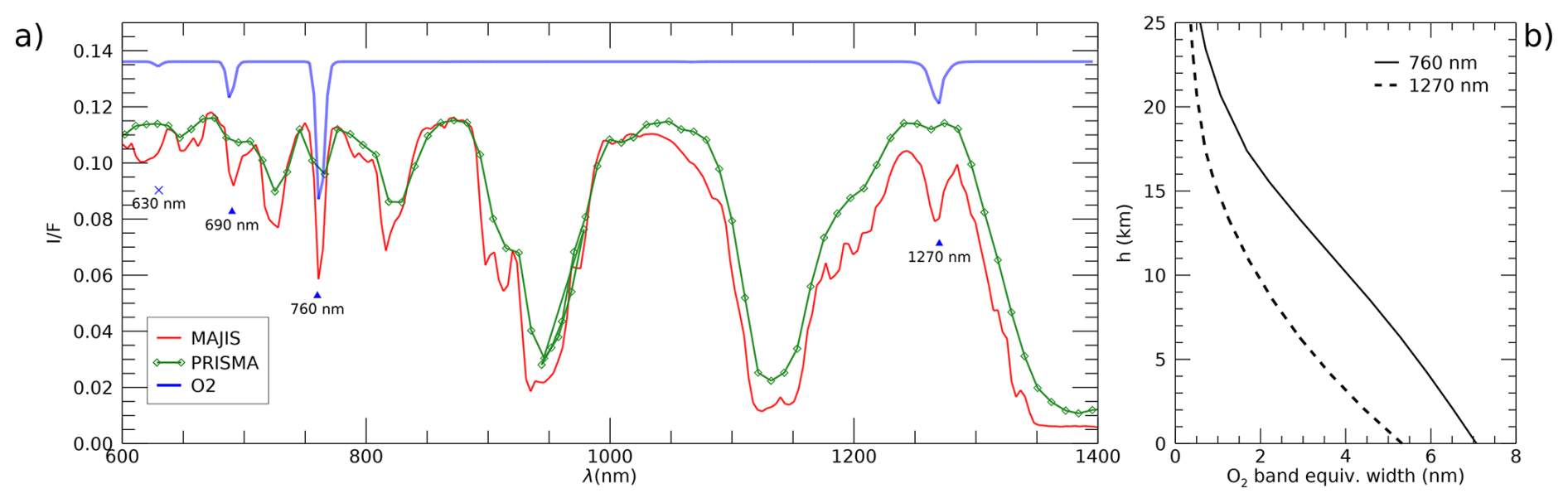
Figure 9 (A) Typical appearance of O₂ features in the spectra of MAJIS (red) and PRISMA (green). Modeled spectral transmittance (in blue) highlights location and shape of the O₂ bands at 630, 690, 760, and 1270 nm. Only the last three can be detected in MAJIS spectra (red curve), while only the strongest 760 nm band is identifiable in PRISMA spectra (red curve). (B) Examples of curves of growth of the O₂ absorption at 760 (solid curve) and 1270 nm (dashed curve) in the standard clear-sky atmospheric column adopted in this work. The absorption is shown as band equivalent width for a 2-ways path with generic incidence and emission angles of 30°.

3.3.2 Cloud shadows analysis

The length of projected clouds shadows gives an estimate of their altitude, provided that the illumination geometry is well known. Significant lengths of projected shadows are more easily seen in the case of tall convective clouds in slant solar illumination. In the MAJIS case, clear shadows have been identified for strong convective events surrounded by widespread background clouds, hence their length can only give hints on relative altitudes (see Sect. 4.2.2). Here we adopted the simplest assumption of homogeneous cylindrical shapes (without accounting for the actual three-dimensional density distribution) to estimate the height of clouds' top with purely geometrical considerations. Under these hypotheses the associated uncertainties are mainly driven by errors in edge detection (for both cloud and shadow edges) and, as a consequence, are limited by the spatial resolution. Errors on solar incidence angle may also play a role in very slant illumination, and the total relative uncertainties estimated in the conditions of MAJIS observations range between 6 and 10 %. The application of the method is shown in Sect. 4.2.2.

3.3.3 Derivation of clouds' altitude with the ice temperature

We apply to Earth's icy clouds the same method by Filacchione et al. (2016), who estimated the temperatures of Saturn's icy satellites surfaces from the displacement of the 3700 nm ice peak, deriving from a shift of the imaginary part of the ice refractive (Mastrapa et al., 2009). In that method, temperature-dependent peak reflectivities were derived from laboratory measurements by Clark et al. (2012), spanning between 88 and 172 K, a range too low to describe Earth troposphere where clouds are commonly observed. We extrapolate the peak-temperature dependence by also simulating the ice reflectivity at 266 K, i.e. the temperature of the optical constants by Warren and Brandt (2008). Since the ice grain size has little effect on the peak position (Filacchione et al., 2012) we assume an effective radius of 20 µm, representative of cirrus clouds (World Meteorological Organization, 1988). The resulting trend covering from 88 to 266 K is shown in Fig. 10 (black and red crosses). It is reliably fit with a second-degree polynomial (green line) and can be used for a qualitative estimation of the ice temperature in MAJIS observations (Sect. 4.2.3).

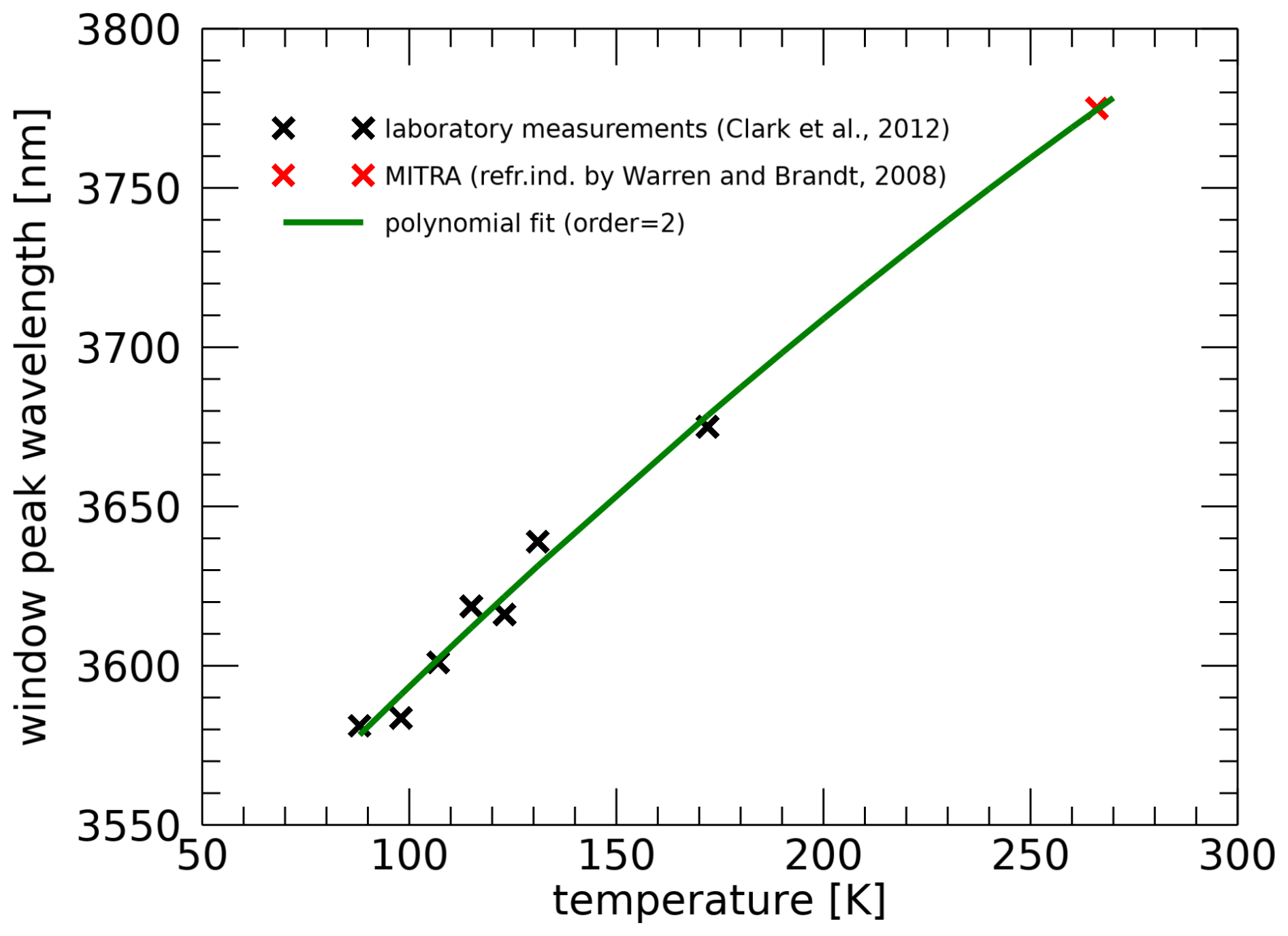
Figure 10 Correlation between ice temperature and 3700 nm reflectivity peak position. Black crosses represent laboratory measurements by Clark et al. (2012), the red cross indicates an RT simulation performed with ice grain size of 20 µm and optical constants by Warren and Brandt (2008), and the green line represents a second degree polynomial fit of all data (see Sect. 3.3.3).

3.3.4 Forward RT modeling on liquid and ice H₂O clouds

The most accurate method for determining clouds' vertical distribution is through full RT modeling. However, this would require a time-consuming retrieval of physical quantities that is beyond the scope of this paper. Instead of spectral inversion, we here perform a comparison of selected observations (i.e., those in Fig. 3) with forward RT models obtained by manually tuning aerosols' physical parameters. The derived quantities are to be considered as orders of magnitude of the altitude and microphysical properties of Earth's clouds and aerosols. Forward models are produced with the MITRA RT tool (Oliva et al., 2016, 2018; Sindoni et al., 2017; D'Aversa et al., 2022), adopting the optical constants from Hale and Querry (1973), Warren and Brandt (2008) and Kitamura et al. (2007) for computing the scattering properties of liquid water, water ice and silicate minerals (assumed as background aerosol), respectively. The spectral albedo of the ocean is taken from the ASTER spectral library (Baldridge et al., 2009). In this simplified scheme, we neglect thermal emission, discarding measurements longwards 3000 nm.

It is interesting to note that, even if beyond the scope of this paper, more accurate RT modeling could also be considered for the evaluation of straylight contamination (studied for MAJIS in Langevin et al., 2026), as it offers the possibility to extrapolate information from the NIR part of the spectrum to visible wavelengths.

3.4 High altitude emissions and atmospheric waves identification

Among the many gaseous features observable in the 4000–5500 nm MAJIS range, two are particularly interesting, being observed as emission bands. These are the CO₂ double-peak at the bottom of the main 4300 nm band and an O₃ signature around 4700 nm. Both are evident above optically thick clouds at high altitudes, blocking the thermal contribution from the surface and lower (hotter) atmospheric layers. The CO₂ peak is radiometrically much more stable than other spectral features against variation of atmospheric structures (see Poulet et al., 2026). It is known to result from the combination of a LTE component induced by temperature increase in the stratosphere, and a non-LTE one due to the CO₂ excitation primarily induced by direct solar pumping occurring at even higher altitudes (where collisional quenching is no longer efficient, e.g. Cassini et al., 2025). The detailed analysis of this emission feature in MAJIS data, implying the evaluation of CO₂ vibrational temperature vertical profiles, is far beyond the purpose of this work. In any case, the spatial distribution of the CO₂ emission intensity can provide interesting insights about the probed layers, and we can indeed use it for detecting atmospheric waves and provide hints about their altitude and propagation (see Sect. 4.3.1). CO₂ emission can be identified already in MAJIS monochromatic frames at 4270 nm (i.e. the position of the main peak of the emission) but the integration of the band in a narrow spectral range is useful for reducing noise and enhancing the contrast in waves' investigation (Sect. 4.3). For the integration we consider wavelengths between 4254 and 4333 nm, which probe high altitudes in the atmosphere and are not affected by the thermal contribution from lower ones. Considering the SNR estimated at these wavelengths (Fig. 3C), we are able to detect waves whose relative intensity between crests and troughs is about 1 %, assuming a 3-sigma uncertainty for the radiance at 4270 nm.

On Earth, ozone has a maximum density in the lower stratosphere but its vertical distribution strongly depends on latitude (see for example Bekki and Lefevre, 2009). It is produced through a very fast and exothermic 3-body recombination reaction that includes O and O₂ in the presence of a catalytic species (either N₂ or O₂). Aside from diagnostic bands at UV (outside MAJIS domain) and VIS wavelengths (the Chappuis band discussed in Sect. 2.3.2), the 4700 nm one is the strongest feature clearly detectable within the MAJIS range. This O₃ band is seen as either an absorption or emission feature in MAJIS nadir-looking observations, depending on the overall thermal emission of the atmospheric column. In clear sky conditions, when the emission from lower warmer layers is dominant, the O₃ 4700 nm band is hardly detectable being overcome by water absorption (as shown in Poulet et al., 2026), unless radiative transfer modeling is performed on the data (e.g. Guerlet et al., 2026). In the presence of mid-altitude clouds, a shallow O₃ band appears in absorption, while the obstruction of the densest part of the atmospheric column due to high-altitude clouds makes the O₃ band appear in emission. Given this phenomenology, in this preliminary study we investigate the O₃ emission amplitude through the difference between brightness temperatures estimated at 4717 nm (strongest O₃ line) and 4660 nm (outside O₃ band). Such a difference is positive when the O₃ is spectrally observed in emission, negative otherwise.

3.4.1 Atmospheric waves characterization

Atmospheric gravity waves are observed in almost all the MAJIS acquisitions (see examples in Sect. 4.3.1) at the wavelengths of the central peak of the 4300 nm CO₂ band. Due to the limited field of view, wave packets are usually not visible in their entirety and it is not possible to identify the same wavy structures from one image to the other due to the large coverage gaps, preventing the study of the wave speed propagation. Nevertheless, we attempt to quantify wave properties and provide some hints on their altitude. The wave parameters – horizontal wavelength, total packet length, azimuthal extent, and packet width – are determined through visually processing each image. Automated methods were not possible because of the variability in images' contrast. After appropriate image stretching, the wavefronts are identified by tracing the crest lines. The horizontal wavelength is defined as the average distance between consecutive crests within each wave packet. The total packet length is measured as the distance between the first and last identified crests. The azimuthal extent is derived from the common orientation of the crests counted counterclockwise, while the packet width is defined as the maximum crest length among those identified. Taking into account spatial resolution and signal contrast, uncertainties in size estimation are of about 7 km, while those on wavelengths are less than about 11 km.

Circular-wave patterns have been observed in some MAJIS images, likely resulting from the breaking of upward-propagating waves originating in sufficiently strong convective thunderstorms. Under this assumption, we attempt to infer the time delay between the wave-triggering event and its observation (Taylor and Hapgood, 1988; Dewan et al., 1998; see Sect. 4.3.1). This is done by neglecting wind transport and assuming a simplified isothermal dispersion relation (Hines, 1960) in which the wave speed is negligible with respect to the speed of sound. For circular waves we also measured maximum radius and expansion speed. Because only a portion of the circle is visible in the images, the wave radius is inferred from the following formula:

$$\begin{array}{}\text{(1)}& r=f/\mathrm{2}+c^{\mathrm{2}}/\mathrm{8}f\end{array}$$

where f is the sagitta and c is the chord, observed in the images in pixels and converted to km using the instantaneous resolution in km per pixel reported in Table 1. The waves are assumed to occur at 15 km height, based on estimations of the brightness temperature of CO₂ emission at 4300 nm, used as a proxy for these features. Following the formulation in Taylor and Hapgood (1988) and Dewan et al. (1998), the wave period τ and expansion speed v_gx can be obtained using the following formulas:

$$\begin{array}{}\text{(2)}& {\displaystyle }{\mathit{\tau }}^{\mathrm{2}}={\mathit{\tau }}_{\mathrm{B}}^{\mathrm{2}}\left[\right(\mathrm{1}+\mathrm{1}/\left(\tan \mathit{\varphi }{)}^{\mathrm{2}}\right]\text{(3)}& {\displaystyle }{v}_{gx}=({\mathit{\lambda }}_x/\mathit{\tau })\cdot [\mathrm{1}-({\mathit{\tau }}_{\mathrm{B}}/\mathit{\tau }{)}^{\mathrm{2}}]\end{array}$$

with ϕ being the elevation angle identified by the wave propagation direction, λ_x= wavelength of the propagating wave, and τ_B= buoyancy period, the latter assumed to be equal to 5 min, which is a good approximation at stratospheric altitude (Dewan and Good, 1986).

4 Results and discussion

We now present the results we obtain through the application of the methods discussed in Sect. 3. Section 4.1 provides a discussion on ice properties, Sect. 4.2 focuses on the clouds' altitudes, Sect. 4.3 is devoted to high altitude features and Sect. 4.4 presents results on land features identification.

4.1 Icy clouds properties

Examples of two MAJIS and PRISMA cubes containing ice clouds, identified through the ice spectral index in Table 3 (threshold <1), are given in Fig. 11. In the MAJIS case, ice is found in localized convective clouds (Fig. 11A and C), so high with respect to the background structures that they even cast well detectable shadows (see Sect. 4.2.2). Instead, in the PRISMA observation ice is detected both in diffuse bright clouds (e.g. at the southern east corner of Fig. 11B and D) and in thinner and less contrasted structures (probably identifiable as high altitude cirrus clouds, e.g. the white regions around longitude 116.4° – latitude 16.5°, Fig. 11B and D) hence proving the effectiveness of the index with different regimes of ice optical depth. Sample spectra from the identified classes are shown in Fig. 11E and F for MAJIS and PRISMA respectively. It must be noted that the very low albedo of the ocean in MAJIS spectrum at visual wavelengths (<1 %) is due to the very slant illumination conditions for the selected observation (incidence angle of about 80° for cube C7, see Table 1). On the other hand, the spectra in the thermal range show consistency with the expected temperature regimes, with very cold ice clouds and the ocean hotter than liquid water clouds.

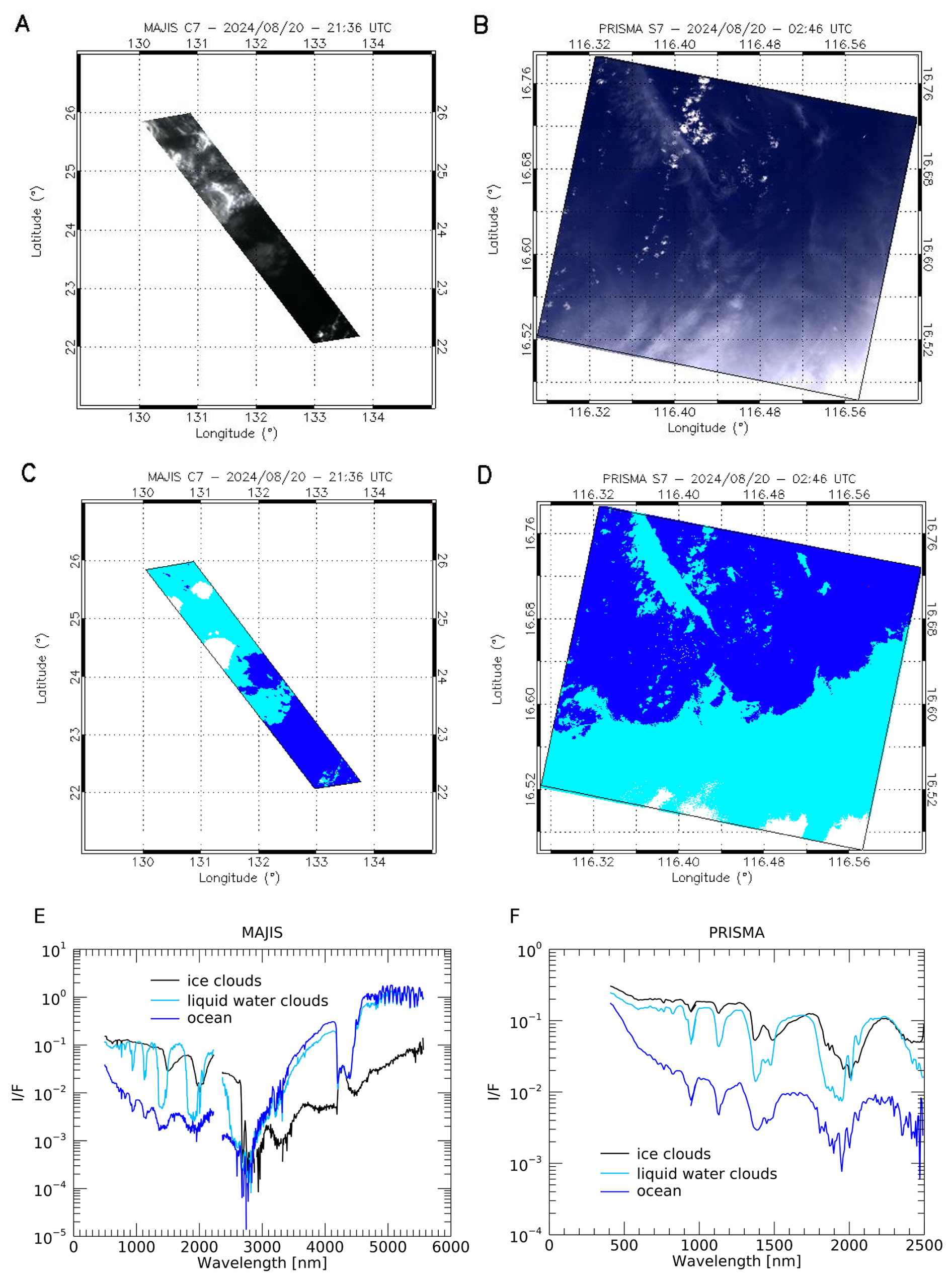
Figure 11 Panels (A) and (B) refer to MAJIS cube C7 and one of the PRISMA cubes from session 07, respectively, displayed in RGB. Panels (C) and (D) show the masks for the detection of ocean (blue), liquid water clouds (cyan, from the “cloudy” condition in Table 3) and ice clouds (white) pixels related to the two cubes. Panels (E) and (F) display sample spectra related to the different classes identified in MAJIS and PRISMA observations.

Ice is similarly widespread in other MAJIS and PRISMA data, so that some considerations on its distribution and correlations between its parameters can be made (Fig. 12). We compute the 1500 nm band asymmetry as a ratio of slopes, the first considered between 1415 and 1500 nm (left wing) and the second between 1500 and 1790 nm (right wing). The asymmetry correlates with the strength of the 1650 nm band (quantified as equivalent width, Fig. 12A and B), with higher values indicating increasingly crystalline ice (Mastrapa et al., 2008; Stephan et al., 2021a; Grundy and Schmitt, 1998). Different regimes of these two parameters map localized structures in MAJIS and PRISMA observations, as shown in Fig. 12C and D respectively where green and blue pixels refer to clusters contained within dashed ellipses sharing the same color in Fig. 12A and B. In MAJIS case, the blue cluster is characterized by an increasing 1650 nm equivalent width at constant 1500 nm band asymmetry. The green cluster, instead, shows a common trend of growth for the two parameters. On the other hand, the PRISMA ellipses identify well separated clusters of points within the two parameters' space.

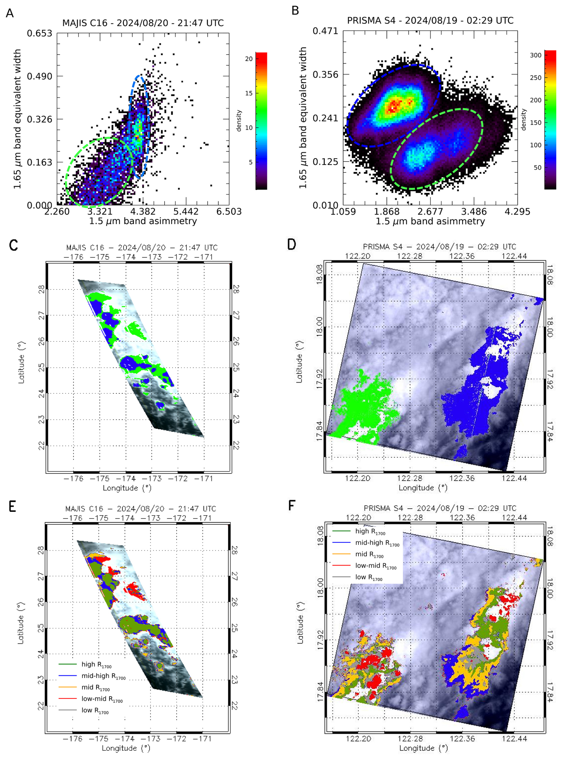
Figure 12 (A–B) scatterplots of the 1500 nm band asymmetry and the 1650 nm band equivalent width for MAJIS reflectance cube C16 and one of the PRISMA reflectance cubes from session 04. The colored-dashed ellipses separate different regimes of the two parameters (see Sect. 3.5). (C–D) green and blue pixels map the clusters contained within the respective ellipses in panels (A) and (B). (E–F) clustering of ice observations, obtained through the K-means classification algorithm (see Sect. 3.2), grouped on the basis of the intensity of the reflectance at 1700 nm (R₁₇₀₀).

It is interesting to note that the correlation between these clusters and those obtained from the K-means classification discussed in Sect. 3.2 (Fig. 12E–F) is not straightforward. For MAJIS, ice spectra with high reflectivity in the solar part of the spectrum (green in Fig. 12E) are mostly correlated with the blue cluster in Fig. 12C. This trend is not observed in PRISMA, where all K-means clusters are equally distributed over both the blue and green clusters shown in Fig. 12D, suggesting variable ice densities and grain sizes within the same regimes of crystallinity. This difference derives from the fact that, as explained in Sect. 3.2, for MAJIS the thermal wavelengths contribute to the K-means classification of the spectra, hence providing information also on the temperature of the ice (see also Sect. 4.2.3). This is verified by the trend of the 1500 nm band asymmetry with the radiance in the thermal part of the spectrum, shown for MAJIS cubes C16 and C17 in Fig. 13A–B: more crystalline ice (larger asymmetry) is correlated with lower radiances (i.e. temperatures) at thermal wavelengths. In particular, orbit C17 also shows a detached cluster in the distribution of the thermal radiance suggesting different regimes of temperature (hence different clouds' altitude). Finally, we show the correlation between the ice crystallinity and its temperature in Fig. 13C–D, where the intensity and wavelength of the Fresnel peak are compared to MAJIS thermal radiances. Consistently with previous studies (e.g. Stephan et al., 2021a), the intensity of Fresnel peak is higher when the temperature is low (Fig. 13C), indicating enhanced crystallinity (see also Poulet et al., 2026). The comparison in Fig. 13D shows two distinct regimes of the peak position, with the short wavelength cluster characterized by a larger spread of the thermal radiance (suggesting an enhanced temperature variability for a less crystalline ice, e.g. Stephan et al., 2021a).

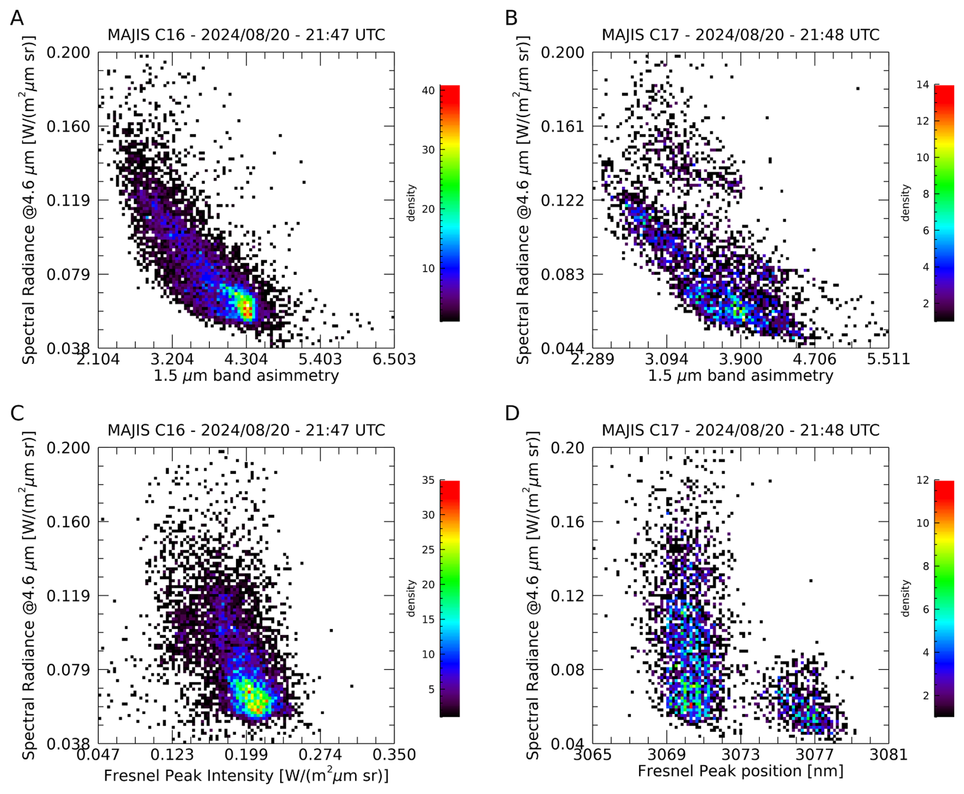
Figure 13 (A–B) scatterplots of the 1500 nm band asymmetry and thermal radiances at 4600 nm for MAJIS orbit C16 and C17 respectively. (C) scatterplot of the Fresnel peak intensity with the thermal radiance at 4600 nm for MAJIS orbit C16. (D) scatterplot of the Fresnel peak wavelength with the thermal radiance at 4600 nm for MAJIS orbit C17.

4.2 Clouds' altitude

We now discuss the altitudes of clouds derived with the different methods presented in Sect. 3.3.

4.2.1 Altitudes from O₂ band depths

Figure 14 shows a comparison of cloud top altitude maps obtained by applying the O₂ bands' investigation method (Sect. 3.3.1) to sample PRISMA and MAJIS cubes. In this case, PRISMA retrievals (Fig. 14A) show two main cloud layers, a higher one between 5 and 9 km (yellow-red colors in the figure, modal value 6.5±1 km) and a lower one between less than 1 and 4 km (blue-cyan colors, modal value 2.0±1 km). MAJIS cloud tops (Fig. 14B), whose model value lies at 4.8±1 km, are in overall agreement with the PRISMA upper cloud deck, even if the observing angles were very different in the two cases (>60° for MAJIS, ∼12° for PRISMA). On the other hand, the population of lower clouds detected by PRISMA appears broken in a series of localized small structures that could remain unresolved if also present in the MAJIS scene (see Sect. 2.3.1). A more systematic discrepancy is obtained when comparing cloud top altitudes retrieved through the 760 nm and the 1270 nm bands (Fig. 14C, shown as reference for MAJIS data only), since the latter gives systematically lower values (most clouds drop below 1.5 km altitude). This discrepancy reflects the smaller sensitivity of this band to higher altitudes and the non optimal modeling assumptions described in Sect. 3.3.1. However, such an issue can be resolved with a more complete radiative transfer modeling as suggested by the benchmark presented in Sect. 4.2.4.

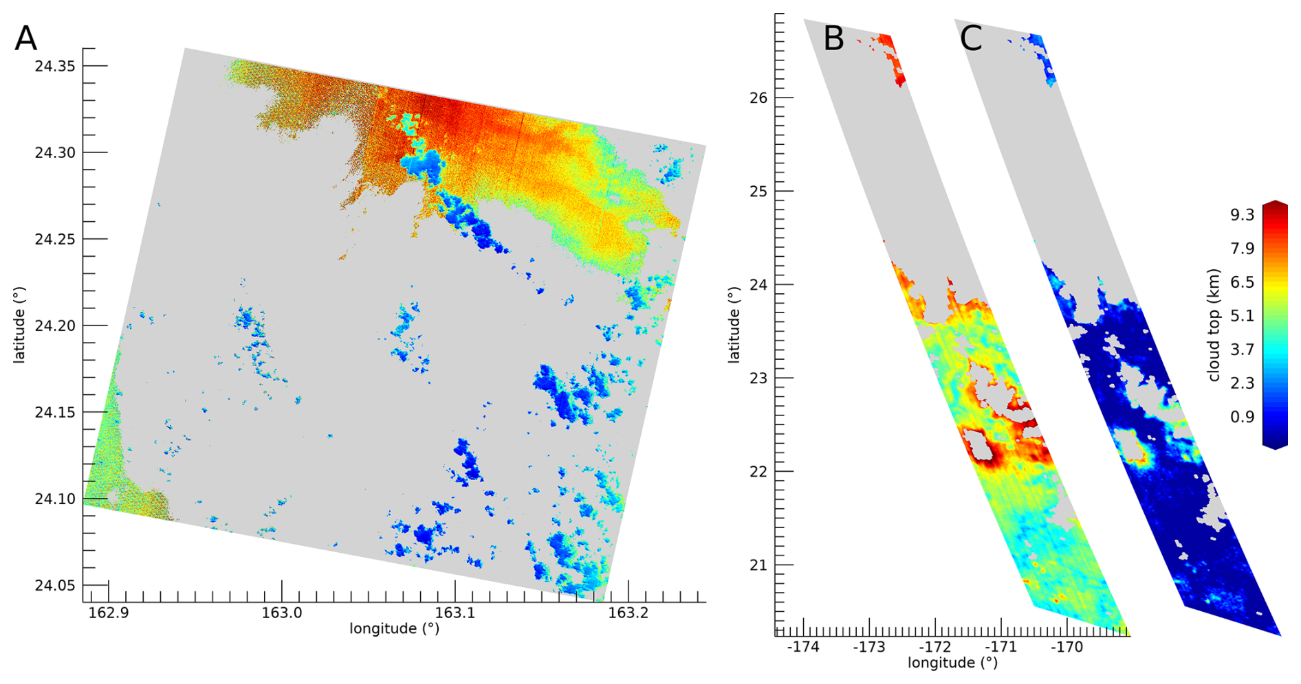
Figure 14 (A) Map of cloud top altitude retrieved through the O₂ 760 nm band in a PRISMA sequence 09 cube (20240820234657). Non-cloudy pixels or saturated ones, excluded from the calculation, are shown in grey. (B) The same as panel (A) but from a MAJIS data cube C17. (C) Cloud top map for the same data in panel (B) (offset for clarity) but retrieved from the 1270 nm O₂ band. Uncertainties are of the order of 1 km (Sect. 3.3.1).

The counts distribution of cloud top altitudes derived from the maps in Fig. 14 is shown in Fig. 15. The altitude ranges of the main cloud deck derived from the O₂ 760 nm band are in good overall agreement between MAJIS and PRISMA (light green and dashed light red curves), characterized by two broad peaks around 4.8 and 6.5 km, respectively. The displacement between these peaks is mainly driven by a true difference in the cloud populations between the two observed scenes, and is further increased by the different spatial/spectral resolutions. A much lower distribution, flattened towards the surface, is indicated by the O₂ 1270 nm band, confirming its scarce usability to trace cloud altitudes. The cloud heights derived from the 3700 nm ice spectral signature (cyan curve) only trace icy pixels of MAJIS C17 cube (see lower panels of Fig. 17 in Sect. 4.2.3) and are distributed, as expected, above the main cloud deck, with a peak around 11 km. The same behaviour is also confirmed by the altitudes distribution evaluated through brightness temperatures' estimation over the same icy spectra (blue curve, 10.5 km peak). The same estimation, applied to non-icy spectra (red curve), gives altitudes significantly biased toward lower levels. This can be mainly ascribed to the fact that the thermal part of the spectrum of thin liquid water clouds observations is affected by an enhanced contribution from the ocean thermal emission. Full radiative transfer calculations would be needed to quantitatively assess this aspect and the assumptions on the specific emissivity of liquid/ice clouds (set to 1 for both in our calculations), but are not performed here as they are beyond the purpose of this preliminary work.

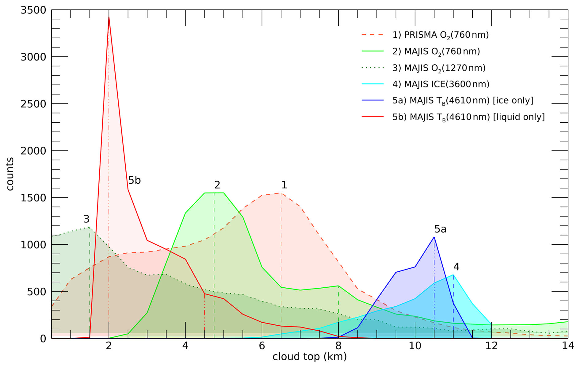
Figure 15 Comparison of cloud top altitudes retrieved from PRISMA and MAJIS session 09 and C17 cubes respectively, through different methods. PRISMA counts are normalized to the maximum value of MAJIS curve 2. Distributions derived from O₂ band depths, related to the maps in Fig. 14A, B, C, are shown in pink (dashed line), light green (solid line), and dark green (dotted line) respectively. Cyan curve refers to ice clouds only (method described in Sect. 3.3.3 and discussed in Sect. 4.2.3), while the distributions obtained from thermal emission at 4610 nm are given separately for water ice (in blue) and liquid water (in red) pixels. The heights of the main distribution peaks are highlighted by vertical dashed lines. Even if the distributions are evaluated in 0.5 km altitude bins, an uncertainty of the order of 1 km must be considered.

4.2.2 Altitudes from clouds' shadows

An example of the results obtained from the method described in Sect. 3.3.2 is given in Fig. 16, where the shadows projected by high convective anvil clouds are clearly visible in MAJIS data cube C7. The grazing illumination of the scene (incidence angle ∼80°) enables a vertical resolution of ∼0.7 km, inferred from uncertainties of ∼0.5° on incidence angles and 2.7 km on shadow length (about twice the horizontal spatial resolution). Within this framework, the horizontal length of the shadow translates to a top altitude of about 10 km (see yellow lines). Of course this value is not absolute but only an estimate relative to the surrounding decks, whose altitudes can be qualitatively inferred through the estimation of the O₂ 760 nm band depth (see previous section). The O₂-derived elevations are shown in the map of Fig. 16B, where the background structures appear to be located around 5–8 km, while the anvil cloud top peaks at ∼16 km. This implies a differential height of ∼10 km between the anvil and the surrounding clouds, in very good agreement with the estimated shadow length. The absolute height of the cloud top can only be derived if multiple scattering effects are accounted for in the reproduction of the 760 nm O₂ band (Sect. 4.2.4). Nevertheless, the shadow analysis provides a quick and independent way for estimating the relative height of isolated structures with respect to their background.

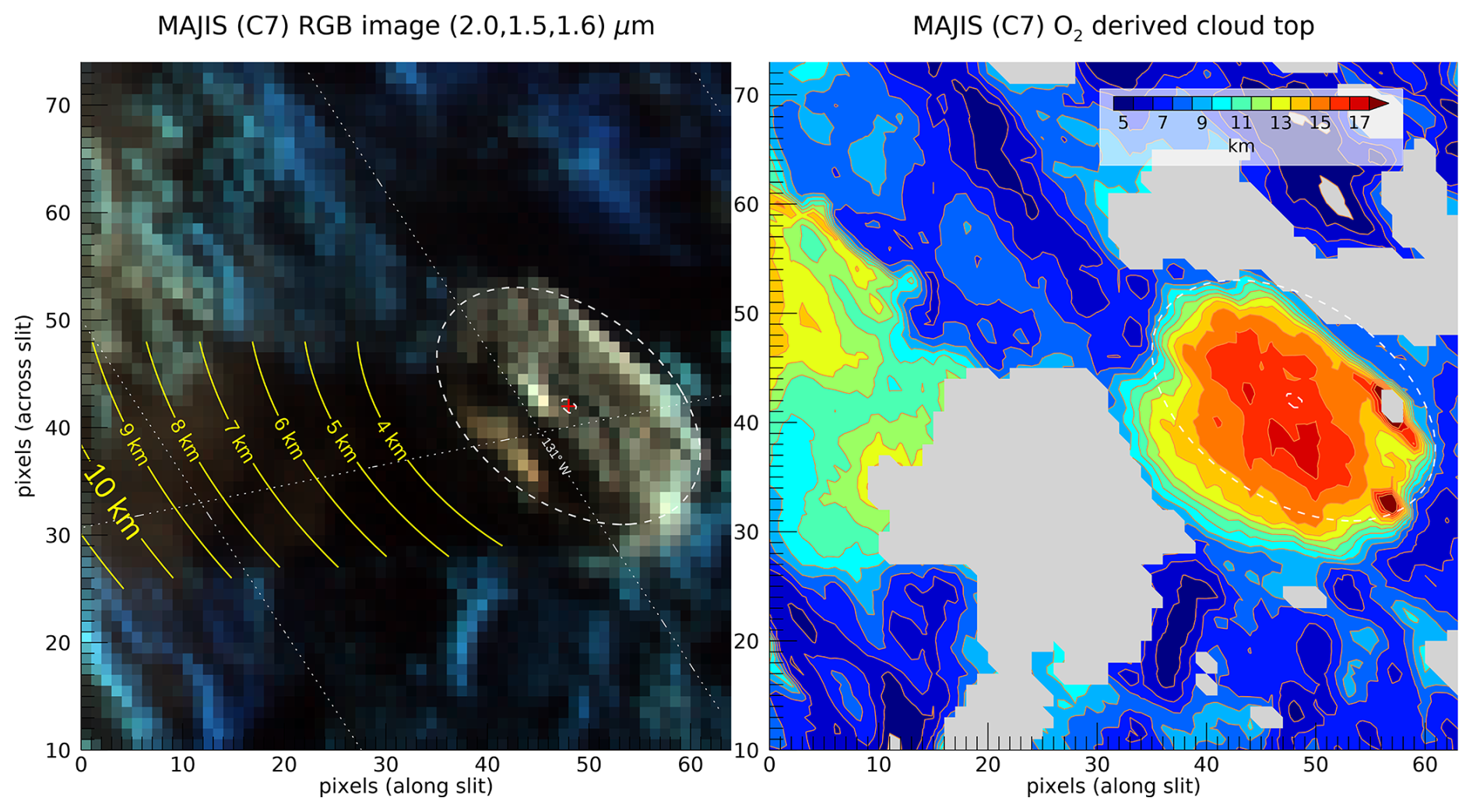
Figure 16 (A) Example of cloud top altitude estimation based on projected shadow length in the MAJIS data cube C7. The white dashed line indicates the approximate boundary of a detached cloud (center indicated by the red dot). The yellow lines show how long the expected shadow would be in the actual geometry by changing the cloud top altitude. The shadow length observed in the background image matches a cloud about 10 km tall. (B) Cloud top altitudes retrieved in the same area from the O₂ 760 nm band (see Sect. 4.2.2), shown for comparison. Gray-filled patches correspond to areas where no O₂ band is measurable.

4.2.3 Altitudes from ice temperature

In Fig. 17 we show two examples of the temperature and altitude maps derived with the method described in Sect. 3.3.3, for MAJIS cubes C16 (upper panels) and C17 (lower panels).

Altitudes are derived by assuming that the clouds are in thermal equilibrium with the surrounding air and reside within the troposphere, where the temperature vertical lapse rate is positive. Altitudes' errors are of about 1 km (Sect. 3.3.1) while those related to temperatures are propagated from the 3700 nm peak uncertainties (Table 4) and result of about 1 K. Orbit C16 shows two main decks, placed respectively at z∼13 km and z∼10 km which can be compared with the maps in Fig. 12C and E, where the 1650 nm band depth and K-means clusters are shown. The higher deck at z∼13 km correlates with the blue cluster in Fig. 12C and the green one in Fig. 12E, suggesting increased opacity and crystallinity at lower temperatures.

Similarly, two regimes of temperatures and altitudes are found in orbit C17, with higher clouds at z∼13 km (T∼205 K) and lower ones at $\mathrm{8}<z<\mathrm{10}$ km ($\mathrm{215}<T<\mathrm{250}$ K). As suggested by the scatterplot in Fig. 13D, these two decks are characterized by different ice properties. Indeed, the short wavelength Fresnel peak cluster (i.e. reduced crystallinity, Cartwright et al., 2025) shows a larger spread of temperatures, consistent with the lower clouds discussed here. Instead, the long wavelength Fresnel peak cluster shows overall lower thermal radiances, and hence temperatures, in agreement with the higher clouds identified at ∼ 13 km (see also Poulet et al., 2026).

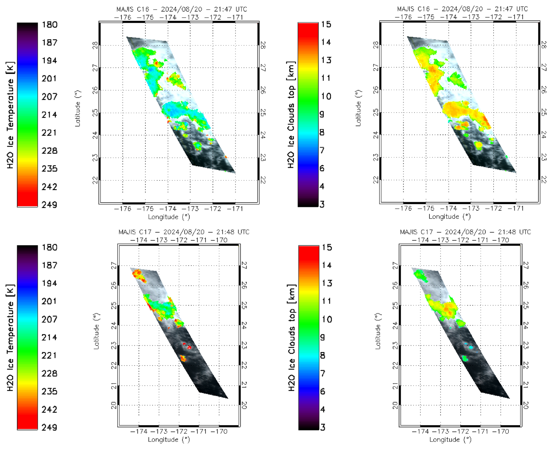
Figure 17 Ice temperature (left) and inferred cloud altitude (right) mapped on MAJIS cube C16 (upper panels) and C17 (lower panels). Ice is identified with a threshold <1 on the ice clouds condition in Table 3.

4.2.4 Results from RT modeling

For our forward RT modeling (Sect. 3.3.4) we consider all MAJIS spectra and the PRISMA liquid water cloud one from Fig. 3, as it is the one showing the most evident differences with respect to its MAJIS counterpart. We also take into account a MAJIS ice cloud spectrum related to one of the convective structures identified in Fig. 11A–C and studied in Sect. 4.2.2.

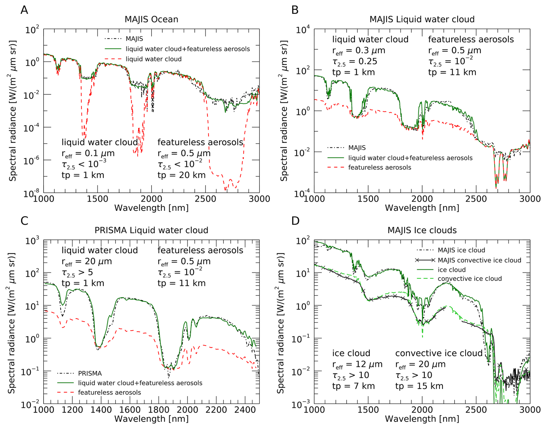
Figure 18 (A) MAJIS ocean spectrum from Fig. 3 is shown in dashed-dot black, its forward RT fit is shown in green, while the contribution from the liquid water cloud in the simulation is given in dashed red. Geometrical and microphysical parameters (r_eff is the effective radius in µm, τ_2.5 is the optical depth at 2.5 µm and tp is the cloud top in km) of aerosols involved in the fit are given in the figure. (B–C) Same as in panel (A), but liquid water clouds observations by MAJIS and PRISMA from Fig. 3 are respectively fit. The dashed red lines here refer to the contribution from the featureless aerosols in the model (i.e. when no liquid water cloud is considered). D: MAJIS ice clouds forward RT fits (green and dashed light green lines) related to MAJIS ice cloud spectrum from Fig. 3 (dashed-dot black) and to a spectrum from the convective cloud identified in Fig. 11C (black line with crosses).

The best fits obtained with this approach are shown in Fig. 18. In general, grain sizes and clouds' altitudes determine the shape and the signal of water absorption bands, while the number density can be tweaked to match the intensity of the continuum. We assume that the clouds are compact in vertical extent and only occupy a single layer of the atmospheric profile. The ocean and liquid water clouds observations require two separate layers placed at different altitudes in the atmosphere (Fig. 18A, B and C) suggesting that, as explained in Sect. 2.3.1 and 3.1, also the ocean spectra we are investigating are partially obstructed by non-resolved cloudy structures. The lower layer shapes the shoulders of water bands', in which the atmospheric transmission is enough to probe down to the surface, while the upper one is needed to correctly model the intensity of the bands' bottom. Indeed, if optically thick enough, high clouds prevent solar photons from reaching the underneath atmospheric layers, hence reducing the gaseous absorption. Such a differential effect in the models is shown as dashed red lines in Fig. 18A, B, C. In the ocean spectrum (Fig. 18A) the optically thin bottom layer (z=1 km, $\mathit{\tau }<{\mathrm{10}}^{-\mathrm{3}}$) with small grain sizes (r_eff=0.1 µm) is consistent with the average properties of maritime droplets ($\mathrm{0}<z<\mathrm{2}$ km, $\mathrm{5}\times {\mathrm{10}}^{-\mathrm{4}}<\mathit{\tau }<{\mathrm{10}}^{-\mathrm{3}}$, $\mathrm{0.05}<r_{\mathrm{eff}}<\mathrm{1.5}$ µm) commonly observed above the surface of the ocean (Croft et al., 2021; Smirnov et al., 2002; Heintzenberg et al., 2000). On the other hand, the upper thin layer ($\mathit{\tau }<{\mathrm{10}}^{-\mathrm{2}}$) has slightly larger particles (r_eff=0.5 µm) and is placed at 20 km, in agreement with the presence of stratospheric background aerosols ($\mathrm{15}<z<\mathrm{25}$ km, ${\mathrm{10}}^{-\mathrm{4}}<\mathit{\tau }<{\mathrm{10}}^{-\mathrm{3}}$, $\mathrm{0.1}<r_{\mathrm{eff}}<\mathrm{1}$ µm, Voudouri et al., 2023; Thomason et al., 2008). Such a configuration confirms the observation as a partially obstructed scenario.

The selected MAJIS and PRISMA liquid water clouds observations (Figs. 3 and 18B–C) show a good radiometric agreement but differences in water bands' shape that can be explained by changes in the aerosols' microphysical properties. Both observations are characterized by a high altitude, spectrally featureless, thin aerosol layer (tp = 11 km, $\mathit{\tau }\sim {\mathrm{10}}^{-\mathrm{2}}$) that is required to reproduce the bottom of water bands. This indicates the presence of faint background stratospheric aerosols residing at the tropopause. Instead, the lower liquid water layer (z=1 km) is thin with small grains in the MAJIS case (τ=0.25, r_eff=0.3 µm) suggesting spray marine boundary layer aerosols (Sun et al., 2024; Zheng et al., 2018; Luo et al., 2014), and thicker with large grains in the PRISMA case (τ>5, r_eff=20 µm), consistent with the presence of stratus clouds (Fu et al., 2022; Rossow and Schiffer, 1999; World Meteorological Organization, 1988). Hence, different properties ensure the modeling of flatter (MAJIS) and sharper (PRISMA) bands in the two observations.

The two ice observations (Fig. 18D) are reproduced with a single cloud layer and do not require the lower one. This is because the ice clouds in the models have opacities so high (τ>10) that they prevent observing the ocean and the atmospheric layers in between. In such conditions, the ice cloud in practice acts as a surface with high albedo, accounting for most of the spectral features in the observations. However, two different clouds' observations are considered here. The first one (black dashed-dot line in Fig. 18D) is related to a small structure identified around longitude 133° and latitude 22° in Fig. 11C. This cloud can be modelled with ice crystals of the order of 10 µm in radius (green line). The altitude can be reliably tweaked by studying the depth of gaseous water absorption bands at 1380 and 2600 nm, both identifiable in the observation. This means that the ice cloud is low enough to ensure some water absorption, before completely shielding the underneath atmosphere. As a result, our estimate is that it has its top at 7 km. These parameters suggest compatibility with the presence of a thick cirrus cloud ($\mathrm{6}<z<\mathrm{13}$ km, τ>3, $\mathrm{10}<r_{\mathrm{eff}}<\mathrm{60}$ µm, Baran, 2009; Zhou et al., 2018; World Meteorological Organization, 1988).

The other ice cloud (black line with crosses in Fig. 18D) is selected on the larger convective structure identified in Fig. 11C. We already expect this to be higher in the atmosphere with respect to the other one (Sect. 4.2.2). Our model (dashed light green line) suggests that it is characterized by larger crystals (20 µm) and reaches an altitude of at least 15 km, enough to prevent water absorption in the 1380 and 2600 nm bands (the model sensitivity to higher altitudes is reduced making this estimate a lower limit). These values indicate that in this observation MAJIS is probing the upper frozen top of a large convective cloud ($\mathrm{8}<z<\mathrm{16}$ km, τ>10, $\mathrm{10}<r_{\mathrm{eff}}<\mathrm{60}$ µm, Dolan et al., 2023; Krisna et al., 2018; van Diedenhoven et al., 2016).

4.3 Upper atmosphere features

The CO₂ and O₃ emissions introduced in Sect. 3.4 have been studied in all MAJIS cubes, deriving maps like those shown in the examples of Fig. 19 and Fig. 20. In Fig. 19, panels (A) and (B) show MAJIS cube C7 displayed at 3100 and 4512 nm, whose anti-correlation highlights the presence of the convective clouds discussed in Sect. 4.1, 4.2.2 and 4.2.4. Panels (C) and (D), instead, show the radiance of the peak of CO₂ emission at 4270 nm and the brightness temperature difference between the O₃ emission peak and its continuum (Sect. 3.4). It is evident how wavy patterns can be seen in the CO₂ map and are uncorrelated with the clouds beneath. No wave patterns are spotted from the O₃ emission, whose positive values (and hence the emission) are only detectable above the convective structures. This suggests that, while both phenomena are likely happening above the clouds' top, waves are generated at different altitudes with respect to those pertaining to the O₃ emission. However, the actual heights are not investigated here, since a rigorous retrieval accounting for non-LTE effects (required for the assessment of these high-altitude emissions) is beyond the scope of the paper.

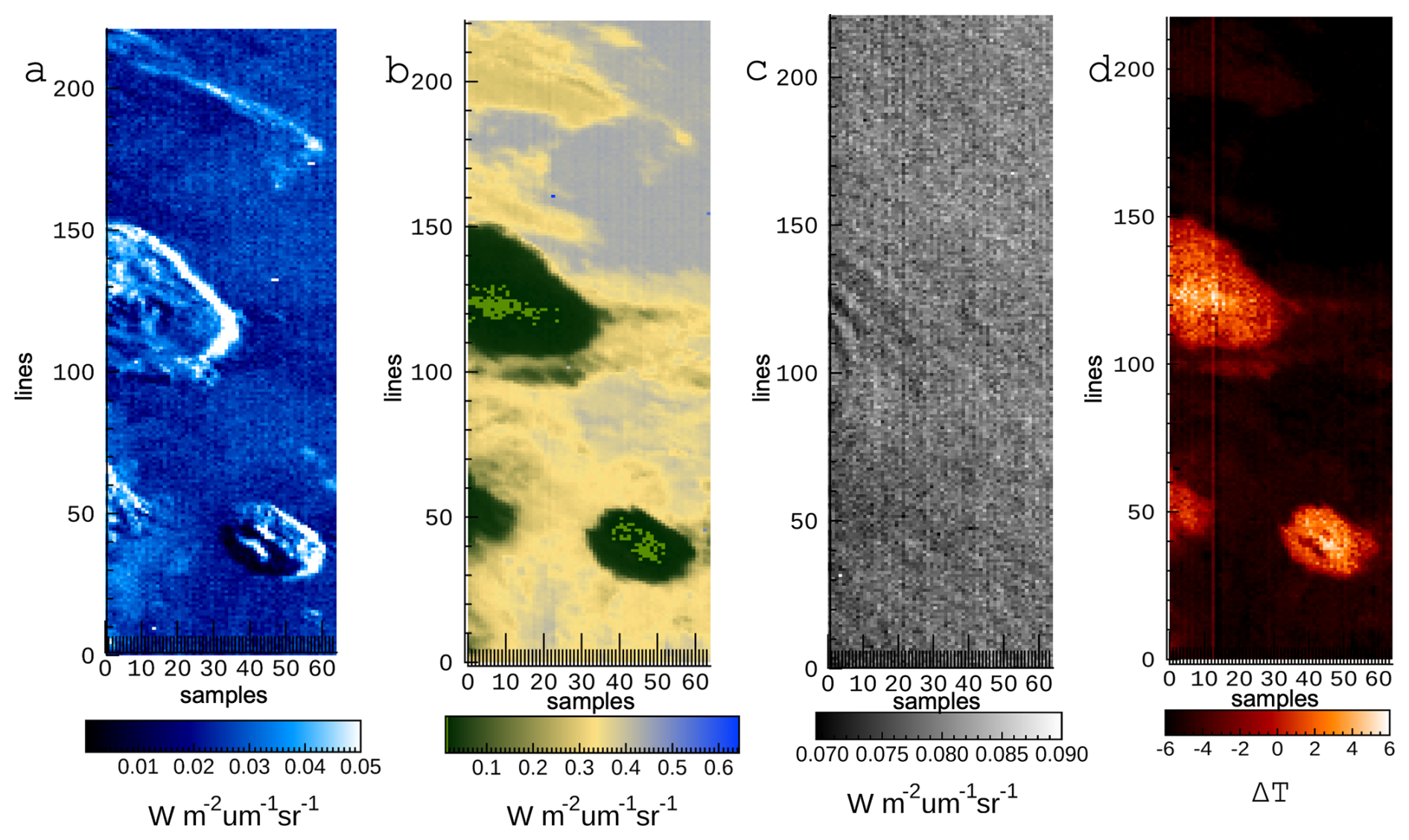
Figure 19 (A–B) MAJIS cube C7 radiances at 3100 and 4512 nm respectively, highlighting the anti-correlation between enhanced ice content (A, i.e. larger reflectances of the Fresnel peak) and low thermal contribution (B). (C) radiance of the CO₂ emission peak at 4270 nm, in which the gravity wave pattern is identified. (D) brightness temperature difference (in K) between the O₃ emission peak (4717 nm) and its continuum (4660 nm), showing positive values above the clouds. In all maps, `samples' and “lines” indicate spatial pixel numbers in the direction along and across the instrument slit respectively.

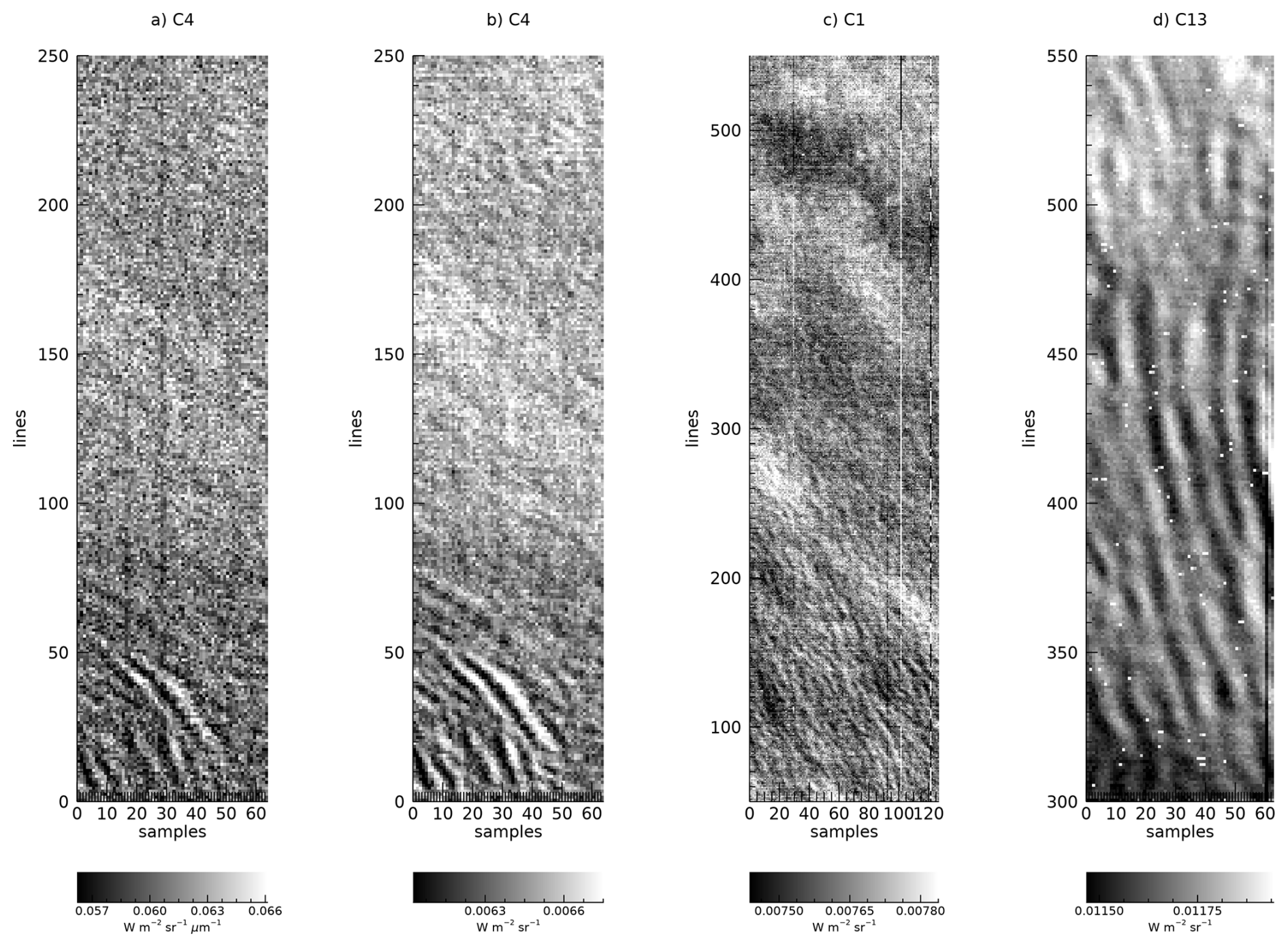
Figure 20 A circular wave pattern is clearly observed in MAJIS C4 cube at 4270 nm (a). Panel (b) shows the enhanced contrast achievable after spectral integration between 4254 and 4333 nm, which also improves detection of complex wave patterns in several MAJIS observations, like in C1 (c) and C13 (d). Pixel scales are reported in Table 1.

Following the discussion in Sect. 3.4, in Fig. 20 we show the effect of the increased contrast that can be achieved through the spectral integration of the CO₂ emission (right panel), with respect to the single wavelength investigation (left panel). The integration reduces noise hence allowing enhanced accuracy in detecting the wave patterns. Indeed, if the radiance integrated in the band is considered, the detectable relative intensity drops from 1 % to about 0.5 %, which translates as an increased capability in characterizing the vertical structure of the waves.

4.3.1 Atmospheric waves properties

Examples of wavy structures identified in the MAJIS images at 4270 nm are provided in Fig. 20. The wave packets have characteristics different from one image to the other in terms of orientations and horizontal wavelengths. In some cases, a curved wavefront is observed (see Fig. 20B, C, D) as well as a superposition between different packets (Fig. 20D).

Table 5 Summary of atmospheric waves parameters (packet length and width, horizontal wavelength and azimuth) calculated from MAJIS data analysis. Columns indicate: image cube, latitude (°), packet length (km), packet width (km), horizontal wavelength (km), azimuth (deg, see Sect. 3.4.1), respectively.

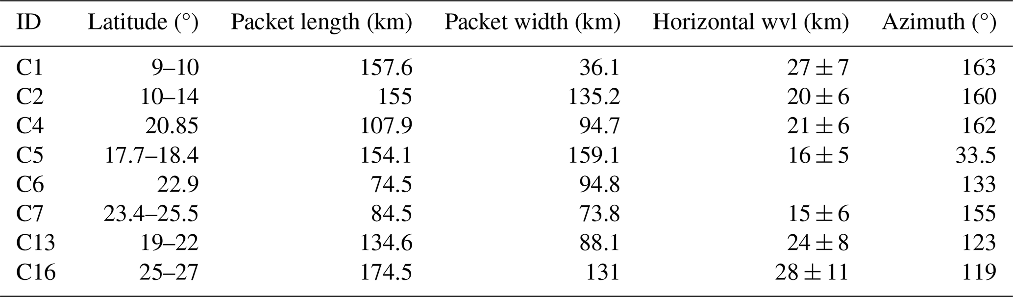
The values obtained from the method described in Sect. 3.4.1 are provided in Table 5. In the observed waves, the measured wavelengths are in the range ∼15–40 km, which can be considered as short wavelengths. Similar waves can be generated by several sources and are usually observed in the stratosphere. According to models, deep convection is the principal source of forcing (Fovell et al., 1992; Piani et al., 2000; Lane and Reeder, 2001) and is also suggested to be responsible for circular wave fronts (alongside isolated thunderstorm events, e.g. as observed from the Midcourse Space Experiment, Dewan et al., 1998). Another source of gravity waves, related to wind flow over mountains, is orography (Fritts and Alexander, 2003; Kim et al., 2003). Depending on the topography, this can generate waves with horizontal scales from a few to hundreds of kilometers (Nastrom and Fritts, 1992; Dörnbrack et al., 2002; Eckermann et al., 2007). However, as the majority of MAJIS EGA observations occurred above open sea areas, a possible origin related to a thunderstorm seems to be more realistic.

For circular waves, we estimate the packets' properties and the time of occurrence of the related thunderstorms (see Sect. 3.4.1). We assume storms occurring at an altitude of 15 km (from thermal brightness estimations) and consider cubes C7 and C4 as examples. The minimum and maximum radii, along with the expansion speed and wavelength derived from the images, are as follows: for cube C7, these parameters are respectively 35 km, 50 km, about 45 km h⁻¹ and 15 km; for cube C4 they are 20 km, 110 km, about 100 km h⁻¹ and 20 km. In both cases, the thunderstorm-triggering events appear to occur approximately 1 h before the corresponding observations. This is compatible with the NASA Worldview archive, where several thunderstorms have been registered over the areas observed by MAJIS at around 05:00 local time. In particular, the wave detection in MAJIS C4 acquisition is located about 80 km far from the coastline, and no significant orographic features are present along the apparent direction of propagation. For this detection, the hypothesis of thunderstorm-generated waves is also strengthened by the intense electrical activity confirmed in D'Aversa et al. (2026), where a lightning event has been detected in the visible range of MAJIS cube C1 through the identification of neutral atomic oxygen and nitrogen emission lines.

4.4 Land features

The land/ocean-contrast detection method described in Sect. 3.1 has been applied to all MAJIS cubes, but only a few land features have been identified. The C1 and C2 cubes, expected to cover large land areas at nighttime, encountered very thick and extended storm systems that prevented any surface visibility. Hence, all observable land regions consist of small islands seen in twilight illumination, colder than the surrounding sea surface but barely observable at visible wavelengths. Besides the largest example (Fig. 7), other islands are found in the cube C5 (Fig. 21): Babuyan (region 3), Sabtang (region 4), and the very small Ibahos island (about 4 km × 2.5 km wide, region 5), all part of the Batanes archipelago. The nearby Dequey island, even smaller (∼0.7 km× 1 km), remains unresolved. With respect to the ocean, the brightness temperatures measured over land and cloud areas (Fig. 21b) are colder, with differences up to ∼6 and ∼8 K respectively. Even if fully located beyond the terminator (solar incidence angle ∼90.8°), a significant signal is detectable also at visible wavelengths, ascribable to light scattering in the upper illuminated portion of the atmospheric column, and to multiple scattering effects in the lower part.

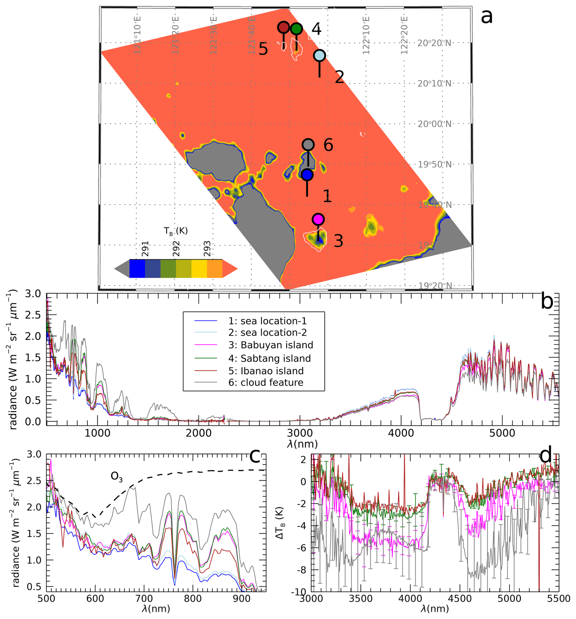
Figure 21 Land spectral features seen in twilight conditions in MAJIS cube C5. (a) Regions of interest (ROIs, labeled 1 to 6) are selected over a 4610 nm brightness temperature map. The coldest areas (in gray) are identifiable as thick clouds, while land areas are slightly warmer (islands of Babuyan, Sabtang and Ibahos, regions 3, 4, 5 respectively), but still colder than the surrounding ocean (red-orange area). Coastlines, obtained from OpenStreetMap under the Open Database License, are shown as white lines. (b) MAJIS full-range spectra over the ROIs. (c) Blow-up of the visible spectral part, showing H₂O and O₂ absorption bands as well as a broad O₃ absorption (see also Fig. 4). (d) Blow-up of the infrared spectral part given as T_B difference with respect to the ocean spectrum.

The MAJIS sensitivity to temperature variations can be estimated from the signal fluctuations over cloud-free ocean regions. The resulting uncertainties in thermal brightness (at 4610 nm) vary between 0.5 and 1 K, which correspond to about 0.2 % and 0.4 % of the radiance at 293 K. This sensitivity appears sufficient to discriminate significant temperature variation not only between sea and land surfaces but also between different land regions. As an example, we show in Fig. 22 the variability of MAJIS brightness temperature inside the Babuyan island, which hosts a volcano of about 1 km in elevation (Babuyan Claro Volcano). Even if the spatial resolution is limited, a clear trend emerges with respect to the topographic altitude, suggesting that the MAJIS data are sensitive to the surface altimetric temperature change.

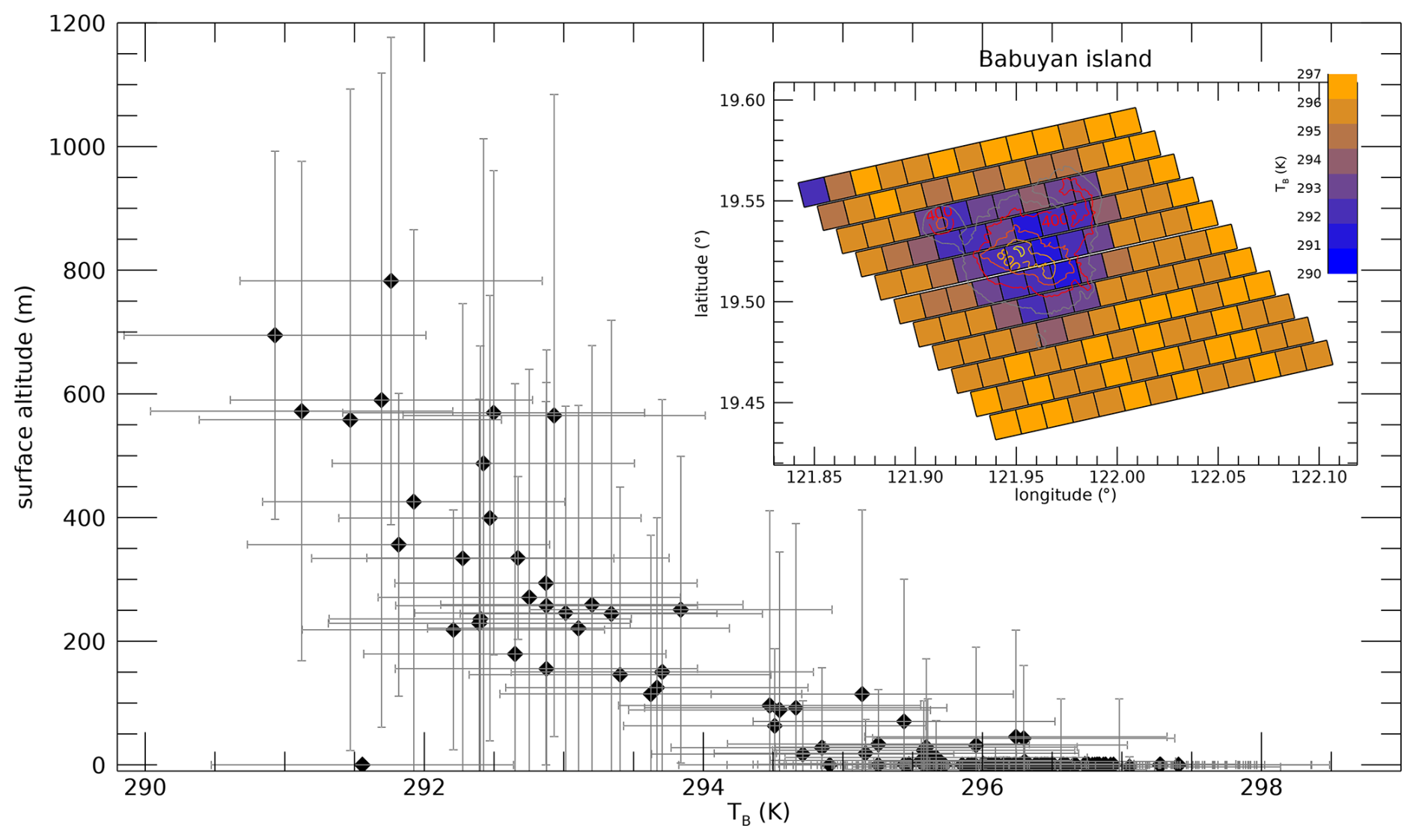
Figure 22 Thermal analysis of Babuyan island, as viewed in MAJIS data cube C5. The MAJIS-derived brightness temperature (at 4610 nm) is plotted against topographic altitude, stressing the detection of surface altimetric temperature change. Error bars on the x axis are derived from signal fluctuation over sea surface around the island, while those on y axis represent the variability of surface altitude inside individual MAJIS pixels. Unit emissivity has been assumed everywhere. Topographic data are extracted from Google Earth Pro 7.3.6.10441 (https://www.google.com/intl/it/earth/about/versions/#earth-pro, last access: 3 September 2025).

5 Application to Jovian system science

This flyby represents the first acquisition of planetary data by MAJIS. Although the analysis presented here has been dedicated to Earth science, we can briefly identify and discuss different links to the MAJIS science that is foreseen at Jupiter and its icy satellites, highlighting the instrument capabilities in exploring different objects of the solar system.

5.1 From ice clouds to icy surfaces

The detection of terrestrial ice clouds described in Sect. 4.1 represents the first spectral observations of water ice performed by MAJIS, and is therefore the first approach to establish the potential outcomes from observations of Jovian icy satellites, in particular for Callisto and Ganymede.

The investigation of ice properties possibly provides information on the differential evolution these bodies underwent in the Jovian system environment. For example, Callisto's surface is mainly covered by crystalline ice, while significant amorphous ice patches have been observed on Ganymede (e.g. Tosi et al., 2024; Bockelée-Morvan et al., 2024; Cartwright et al., 2024). These regions could indicate alteration through radiolysis induced by the impinging of charged particles on the ice (Khurana et al., 2007), hence providing information on the mechanisms connecting Jupiter's magnetic field lines and the moons' surfaces. Moreover, while Callisto is characterized by an overall low ice content on the surface (∼50 %) and presents a more ancient and stable scenario (Greeley et al., 2007), Ganymede's fresh ice patches are indicative of more frequent ice resurfacing and cryo-volcanism events (Ligier et al., 2019). Smaller ice crystals are observed at the poles, matching the distribution of the fresher ice deposits and hence acting as a tracer of geologic activity. In this view, the investigation of ice-related spectral parameters can be used to address many scientific goals of the JUICE mission (Stephan et al., 2021b; Poulet et al., 2024b).

5.2 Clouds

Jupiter's atmosphere is thought to be dominated by the presence of three main cloud decks residing at different altitudes and mixed by convective processes and atmospheric circulation (Fletcher et al., 2023). From lower to higher heights these are respectively composed of a H₂O-NH₃ liquid solution, NH₄SH solid aggregates, and NH₃ ice crystals (Atreya et al., 1999). In particular, the NH₄SH and NH₃ clouds can be responsible for the chromatic differences in Jupiter's dark “belts” and bright “zones”. Above these structures, hazes composed of products of the photochemical disruption of CH₄ and NH₃ extend from the upper troposphere to the stratosphere (e.g. Sindoni et al., 2017; Biagiotti et al., 2025). Such cloud complexity is not present in Earth's atmosphere where water is the only condensible, aside from a variety of aerosols of different origin (e.g. maritime, volcanic, smog, stratospheric). Nevertheless, the study of EGA observations allows a first MAJIS data analysis devoted to disentangling the spectral information related to different sources, like gases, clouds and, in this case, also surfaces. In this manuscript we have investigated clouds under different points of view, including their detection, water vapour phase identification, vertical structure assessment, and microphysical properties estimation. All these techniques are applicable to Jupiter once adapted to the different composition and structure of the giant planet. For example, the RT modeling presented in Sect. 4.2.4 only dealt with the solar part of the spectrum, which would only allow the investigation of Jupiter's hazes and the NH₃ deck (e.g. the recent work of Biagiotti et al., 2025, on JUNO/Jiram data). The exploitation of the full MAJIS spectral range, including thermal wavelengths, is instead mandatory for characterizing the deeper NH₄SH (Grassi et al., 2021) and H₂O (Bjoraker et al., 2022) clouds, especially in “hot spot” regions.

The shadow technique for measuring cloud heights, commonly applied in planetary high-resolution imaging analysis, is also applicable to Jupiter (e.g. Orton et al., 2017). For instance, in observations acquired at the bottom of methane bands, Simon et al. (2015) were able to measure shadows 45 km long, revealing wavy structures less than 1 km in amplitude. In principle, MAJIS observations of Jupiter atmosphere will allow the application of this technique to limited cases, mostly near the terminator and in polar regions when observed from perijove. Maximum spatial resolutions of ∼120 km per pixel achievable in these conditions may enable detecting shadows related to vertical displacements of the order of 10 km.

5.3 High-altitude emissions

The use of chemical atmospheric species as tracers for the atmospheric circulation, including wind measurements and wave detections, is widely applied to the investigation of both terrestrial (i.e. Hueso et al., 2008; Peralta et al., 2008) and giant planets (i.e. Müller-Wodarg et al., 2019; Grassi et al., 2020). A similar approach is valid for the upcoming MAJIS measurements at the Jovian system, whose upper atmospheric dynamical structure can be investigated through the monitoring of the distribution (in latitude and local time) of minor widespread species like H${}_{\mathrm{3}}^{+}$ and hydrocarbons deriving from the photolysis of methane (see Miller et al., 2020, for a thorough review) as demonstrated from both ground-based (see for example O'Donoghue et al., 2016) and space-based data analyses (e.g. Moriconi et al., 2020). MAJIS IR channel will allow to spectrally discriminate the CH₄ and H${}_{\mathrm{3}}^{+}$ contributions in the range 3000–4000 nm, where the two species present strong features (Castagnoli et al., 2025) identifiable within the fundamental 3300 nm CH₄ absorption band, similarly to the case of the 4300 nm CO₂ band in Earth's atmosphere (see Sect. 4.3). The study of CH₄ and H${}_{\mathrm{3}}^{+}$ (e.g. JWST data analysis, Melin et al., 2024) will give access to upper atmospheric layers which are hardly probed otherwise. Altitudes from about 200 km above the 1 bar level are typical of methane emission peak, while above 500 km the H${}_{\mathrm{3}}^{+}$ emission seems to dominate, as also shown by recent analyses of JIRAM-Juno data (Migliorini et al., 2023), where the two species have been spatially separated.

6 Summary and conclusions

In this work we compare the observations of the MAJIS spectrometer on board the JUICE spacecraft, acquired during the Earth gravity assist of 2024 (Sect. 1), with those registered by the Italian Space Agency-led PRISMA spectrometer (Sect. 2). While no exact temporal-spatial coincidence could be achieved, the comparison allowed testing MAJIS spectral and radiometric response over ocean and clouds, the main targets observed during this flyby. Clouds observations have been analyzed for the estimation of altitudes and microphysical properties exploiting different methods (Sect. 4.2). Ice has been detected in most of the observations, allowing a first benchmark of the study of its spectral properties (Sect. 4.1) in view of Jupiter's icy satellites' exploration.

High-altitude emissions from CO₂ and O₃ are also observed in MAJIS dataset, revealing the presence of a significant number of atmospheric gravity waves, whose properties have been derived (Sect. 4.3).

While we discuss ad hoc spectral indices for the identification at VIS-NIR wavelengths of different types of surfaces (in view of the next JUICE Earth flyby happening in September 2026) our investigation of land features is limited to the land/ocean temperature contrast or to the changing surface altimetry (Sect. 4.4). Indeed, in the MAJIS 2024 EGA data no land areas have been captured in daylight.

This wide variety of scientific applications is finally put in the context of the Jupiter case, taking into account the differences between our planet and the gaseous giant's atmosphere and icy satellites (Sect. 5).

In conclusion, EGA data provide the first scientific benchmark of MAJIS instrumental response in a planetary environment, and give the first glimpse of the amount and quality of spectral information we can expect in the Jovian system.