
the Creative Commons Attribution 4.0 License.
the Creative Commons Attribution 4.0 License.
 | 18 Nov 2026
Bursty bulk flow ionospheric impacts from triple-conjunctive observations

Andrew P. Dimmock
Vanina Lanabare
Heikki Vanhamäki
Ilkka Virtanen
Anita Aikio
Adrian Blagau
Octav Marghitu
Milla Myllymaa
Habtamu Tesfaw
Stephan Buchert
Mykhaylo Shumko
Substorms are the regular reconfiguration of the Earth's geomagnetic space environment, and magnetosphere–ionosphere coupling is integral to the substorm chain. Bursty bulk flows (BBFs) are mesoscale fast plasma flows that are released from magnetic reconnection sites in the magnetotail during substorms, and they couple to the ionosphere through field aligned current (FAC) systems. BBFs may drive localised changes to the ionospheric plasma, such as velocity flows or changes to the local temperature, density and conductivity, but determining the specific ionospheric effects of a given BBF and their associated FAC is a complex undertaking. In this study we identify triple-conjugate observations of BBF detections within the magnetotail, FAC observations in low Earth orbit and ground-based radar stations that observe the local ionospheric plasma in order to evaluate the different components of the coupled BBF-FAC-ionosphere system. We evaluate over 11 000 BBFs and identify only 13 events that satisfy our conjunctive criteria, which correspond to 11 unique BBFs. We perform detailed analysis of one of these BBFs, which occurred in the recovery phase of a relatively weak substorm, to evaluate the FAC associated with this BBF and its ionospheric impacts. Multiple FAC signatures were observed that are likely associated with the BBF, in addition to variations in the ionospheric velocity and temperature. There is an ongoing need for coordinated observations of the coupled BBF-FAC-ionosphere system to further distinguish the ionospheric impacts of BBFs from broader substorm dynamics.
- Article
(13022 KB) - Full-text XML
- BibTeX
- EndNote


Substorms are a regular magnetospheric process that drive system-wide changes in magnetic topology to redistribute energy and mass throughout the magnetosphere and across different regions of geospace (Akasofu, 1964; McPherron, 1979). Substorms are initiated by magnetic reconnection in the magnetotail (Angelopoulos et al., 2008a) and are characterised by intense auroral activity within the Earth's ionosphere that has typical duration of a few hours (Akasofu, 2023, and references within). Magnetic reconnection during substorm onset generally occurs around X≃ 20–30 RE in geocentric solar magnetosphere (GSM) coordinates (McPherron, 2016, and references within), where 1 RE = 6371 km is the Earth's radius. Bursty bulk flows (BBFs) are ejected from magnetotail reconnection sites (Ohtani et al., 2004; Birn et al., 2011; Wiltberger et al., 2015) and are responsible for the majority of the Earthward transport of mass and energy from the reconnection site (Angelopoulos et al., 1994). BBFs are mesoscale structures, with typical spatial scale on the order of ΔY = 1–3 RE (Sergeev et al., 1996), that propagate through the central plasma sheet in distinct ion flow bursts that reach velocities of 100's km s−1. Individual BBFs may contribute ∼ 1 % of the total energy deposited into the ionosphere during substorms, and the simultaneous presence of multiple BBFs within the magnetotail (George et al., 2026b) results in BBFs contributing up to 10 % of the substorm energy deposition to the ionosphere (Ohtani, 2019). BBFs therefore play an important role in magnetosphere–ionosphere coupling and the overall transport of mass and energy through geospace during substorms.
Magnetospheric current systems are fundamental to magnetosphere–ionosphere coupling during substorms (Akasofu, 2023), and these current systems also provide a coupling mechanism between BBFs and the ionosphere. The BBF generates flow vortices and magnetic shear on its flanks as it propagates through the plasma sheet, which then establish field aligned currents (FAC) on each flank of the BBF (Birn et al., 2004; Yu et al., 2017). The FAC on the dawnward (duskward) flank of the BBF flows towards (away from) the Earth (Nakamura et al., 2001b; Liu et al., 2015) and these FAC segments on each flank of the BBF close through the ionosphere. The current system associated with BBFs can drive magnetic field fluctuations on the Earth's surface (Wei et al., 2021). FACs can drive convection vortices in the ionospheric plasma, with clockwise (counterclockwise) vortices corresponding to upward (downward) FAC in the Northern Hemisphere when viewed from above (Munsami et al., 2002). The FAC is carried by electrons that propagate along the magnetic field line, so the anti-Earthward portion of the BBF's FAC system is carried by electrons that are propagating towards the Earth. The electron precipitation associated with the upward FAC on the flank of the BBF can also drive auroral streamers, which are narrow, transient structures that originate in the poleward oval and propagate equatorward over time (Nakamura et al., 2001a; Sergeev et al., 2004; Pitkänen et al., 2011; Yang et al., 2025).
There are multiple possible ionospheric signatures of BBFs and their associated auroral streamers. Pitkänen et al. (2011) showed from EISCAT radar and optical measurements that quiet-time BBFs are associated with auroral streamers that start from the vicinity of the polar cap boundary, intrude equatorward, brake at 68–70° MLAT and drift westward along the oval. The ionospheric plasma flow within and poleward of the auroral streamer evaluated in Pitkänen et al. (2011) had an equatorward component. This equatorward ionospheric flow is consistent with the Chen and Wolf (1993) model of the BBF as a component of an underpopulated flux tube that is coupled to the ionosphere in each hemisphere. In this model, Earthward propagation of the BBF corresponds to a contraction of the flux tube, which would then drag the ionospheric footpoints of the flux tube toward the equator to generate an equatorward ionospheric flow channel. A mesoscale flow channel in the nightside ionosphere was observed to be associated with enhanced ion temperature and decreased electron density using radar observations (Aikio et al., 2018), indicating that ionospheric plasma flows may drive localised changes in ionospheric plasma temperature and density. The ionospheric equivalent current signatures of BBFs in the Northern Hemisphere are narrow channels of northwestward equivalent current density: these channels are oriented in the geomagnetic southeast-northwest direction (Juusola et al., 2009). Downward FAC typically occurs at the northeastern flank of these flow channels, with upward FAC occurring on the southwestern flank (Juusola et al., 2009). Lanabere et al. (2026) evaluated the ionospheric currents and auroral activity in response to six consecutive BBFs, using ionospheric current density that was derived from magnetometer observations across Fennoscandia (the region containing the ionospheric footpoints of the BBFs), and demonstrated fast, structured responses of the ionospheric currents to the BBFs that cumulated in the emergence of a strong westward electrojet. Analysis of a hybrid-Vlasov simulation of the Earth's magnetosphere with a coupled ionosphere additionally demonstrated that BBFs can locally increase the conductance of the ionospheric plasma (Workayehu et al., 2025).
Untangling the ionospheric impacts of BBFs and the associated energy transfer mechanisms is a complex undertaking. BBFs originate from magnetic reconnection sites, which inherently means that they occur during geomagnetically active conditions, so it is non-trivial to isolate the impacts of a given BBF from general substorm dynamics. Furthermore, the large spatial scales associated with this process means that no single satellite constellation or ground-based observatory is capable of observing a BBF, the FAC that couples that BBF to the ionosphere and the local ionospheric plasma at the magnetic footprint of the BBF. This study builds on the analysis presented in Lanabere et al. (2026) by evaluating the ionospheric dynamics that are immediately local to the magnetic footprint of a single BBF, which we perform in conjunction with FAC observations. We evaluate a case study of a BBF that occurred during the recovery phase of a relatively weak substorm in order to, as much as possible, distinguish the effects of the BBF from the broader substorm activity. Section 2 presents the data that was analysed in this case study and Sect. 3 describes the methodology used to identify triple-conjugate events. The results of the case study are presented in Sect. 4. The discussion is in Sect. 5, and Sect. 6 summarises the conclusions of this study.
The Time History of Events and Macroscale Interactions During Substorms (THEMIS, Angelopoulos et al., 2008b) is a National Aeronautics and Space Administration (NASA) mission that was launched in February 2007. The THEMIS mission originally consisted of five identical satellites, labelled A–E, on elliptical orbits around the Earth with apogee of ∼ 12 RE; two of the satellites (B and C) were diverted to lunar orbit in 2012. We use data from THEMIS-A, D and E in this study. THEMIS ion observations are obtained from the Electrostatic Analyser (ESA, McFadden et al., 2008) and Solid State Telescope (SST); ESA observations span the 10 eV–25 keV range and SST observes the 25 keV–6 MeV ion population, and these are combined into the ground moments (GMOM) data product. Magnetic field data are obtained from the fluxgate magnetometer (FGM, Auster et al., 2008) observations.
The European Space Agency's (ESA's) three-satellite Swarm mission (Friis-Christensen et al., 2006) is the first multi-point mission to the ionosphere, launched in November 2013. Two Swarm satellites, A and C, travel side by side at an altitude of about 460 km, with a nominal angular separation between their orbital planes of 1.4° and an along-track separation between ∼ 4–10 s. The third satellite (Swarm B) samples the ionosphere at a slightly higher altitude of ∼ 510 km. Swarm-B also has a slightly different orbital inclination than Swarm-A and -C, setting a relative drift of ∼ 22.5 ° yr−1 with respect to the orbital planes of the lower satellites. In this study, we use both the low resolution (1 Hz) and the high resolution (50 Hz) Level 1b magnetic field data provided by the Vector Field Magnetometer (VFM). The single spacecraft FAC density estimates were obtained using the SwarmFACE package (Blagau and Vogt, 2023). Although for the analyzed event the differences with respect to the standard Level 2 FAC density are negligible, the new algorithm (integrated in the MS-MVA tool, see below) deals in general better with the intervals of missing or corrupted magnetic field data and enables pre-filtering of the magnetic field data, which is useful for e.g. the study of FAC structures at different spatial scales.
The magnetic perturbation is derived by subtracting the CHAOS-8 model data (Kloss et al., 2026) from the observed magnetic field and presented in the North-East-Center (NEC) coordinate system, whose axes point northward, eastward, and to the center of the Earth. The magnetic perturbation is subject to the multi-scale minimum variance analysis (MS-MVA; Bunescu et al., 2015, 2019; Bunescu, 2024). In addition to standard MVA results (Sonnerup and Scheible, 1998), namely planarity and inclination with respect to the East direction, MS-MVA provides also information on the location of the FAC structures as well as on their transverse and longitudinal scales (along the maximum and intermediate variance directions, respectively).
The Poker Flat Incoherent Scatter Radar (PFISR), located at the Poker Flat Research Range (PKR) near Fairbanks, Alaska (65.13° N, 147.47° W), is an incoherent scatter radar using the Advanced Modular Incoherent Scatter Radar (AMISR) technology (Nicolls and Heinselman, 2007; Heinselman and Nicolls, 2008). Its phased-array antenna and solid-state transmitters allow for electronic beam steering on pulse-by-pulse basis, enabling simultaneous observations in multiple look directions (Heinselman and Nicolls, 2008). Electron number density, electron temperature, ion temperature, and line-of-sight (LoS) plasma bulk velocity are measured at a number of altitudes along each radar beam direction. These data are available at the MADRIGAL database (Bhatt, 2018) with 1 min integration time. During 31 January 2018 event PFISR was operated in an 11-beam mode called WorldDay40, with nine beams looking northward of the radar and forming a 3-by-3 array in magnetic latitude and longitude, with additional vertical and field-aligned beams. Illustration of the beam pointing geometry is available from the Madrigal database (Bhatt, 2018). The radar mode uses both uncoded long pulses (330 µs) and alternating codes. We use plasma parameters inverted from the long pulse data, because they provide better signal-to-noise ratio and sufficient spatial resolution in the F region. The plasma flow vectors are estimated using the method by Tesfaw et al. (2025), where a local electrostatic electric field model is fitted to the F-region LoS data measured between 200–400 km altitude assuming a perfect E-cross-B drift and equipotential field lines. Each time step is analyzed independently and the LoS data are weighted by their estimated uncertainties. The fit is stabilized using zeroth-order Tikhonov regularization.
A digital all-sky imager at PKR includes filters for 428, 558, and 630 nm emissions (Lynch et al., 2015; Blinstrubas et al., 2025). The images for each filter are taken every 12.5 s. The green line 558 nm images were projected on a geographic map assuming 110 km emission altitude, and are combined with the PFISR plasma flow velocity estimate to study motion and evolution of the auroral structures during the event. We note that calibration data was not available for the event in question, so calibration for the year 2016 was used in the map projection. The optical observations were aided by a fortuitous lunar eclipse during the BBF evaluated in this case study. SuperMAG ground-based magnetometer data (Gjerloev, 2009, 2012) are also used to supplement the THEMIS, Swarm and PKR observations. We specifically use data from the Barrow (BRW), College (CMO), Dawson City (DAW) Deadhorse (DED), Eagle (EAG), Fort Yukon (FYU), Gakona (GAK), Kenai College (T55) and Kiana (T41) stations, which are all located in Alaska.
We evaluate triple conjunctions between BBF detections in the Earth's magnetotail, Swarm satellites in the ionosphere and ground-based radar stations using BBF observations detections from 2017–2024. We use an existing databases of BBFs identified in George et al. (2026b) from THEMIS observations. The BBF identification algorithm in George et al. (2026b) was triggered when the ion velocity magnitude exceeded location-dependent threshold velocity, defined as vthresh = (10d+50) km s−1 (where d is geocentric radial distance in RE) and , while THEMIS was within the magnetotail, defined as X≤ − 5 RE, geocentric radial distance in the XY plane ≥ 8 RE and within the Lin et al. (2010) magnetopause model calculated with Pdyn = 20 nPa and Bz = 0 nT. The duration of the BBF was then defined as the time period that the ion velocity magnitude was greater than , and events that were less than 10 min apart were defined to be a part of the same BBF. These identification criteria allowed for either tailward or Earthward propagation of the BBFs, but Earthward propagating BBFs are expected to have the greatest ionospheric impacts. We therefore impose two additional criteria to ensure that the Earthward motion of the BBF dominates its propagation:
-
max(vx)≥ 100 km s−1
-
|max(vx)|≥|min(vx)|
Criteria 1 ensures that there is sufficiently large Earthward propagation while criteria 2 requires that the Earthward motion is larger than any tailward propagation, as it is not uncommon for BBFs in the braking region to undergo flow reversal and have both Earthward and tailward components. The maximum and minimum values of vx are taken in GSM coordinates from the ion velocity observations provided by the ESA instrument over the duration of the BBF. Following the application of these additional criteria, we have a database of 2642 (3037, 3013) BBFs identified by THEMIS-A (D, E) between 2017 and 2024.
We compute the footpoint of each BBF using four Tsyganenko models (Tsyganenko, 1989, 1996, 2002a, b; Tsyganenko and Sitnov, 2005); these models are referred to as T89, T96, T01 and T04, respectively for the remainder of this manuscript. These are all empirical, data-based models of the magnetic configuration of the Earth's magnetosphere. The T89 model provides a magnetospheric model with a warped magnetotail current sheet, which is based on observations by 10 satellites of the magnetic field from 1966–1980 in the geocentric distance range from 4–70 RE; the T89 model requires only the geomagnetic index Kp as input. The T96 model extends on T89 through the explicit inclusion of a solar-wind-controlled magnetopause and effect of reconnection at the magnetopause, and inclusion of the Birkeland current systems. The T96 model is based on magnetic field observations from 11 satellites from 1966–1986 at geocentric radial distance from 4–60 RE (Fairfield et al., 1994), and this model uses the geomagnetic index Dst, solar wind Pdyn and interplanetary magnetic field (IMF) BY and BZ as inputs. The T01 model incorporates a dawn-dusk asymmetry with an improved mathematical representation of the Birkeland, ring, and cross-tail current systems, and this model specifically focuses on the inner magnetosphere (X≥ −15 RE). It is based on magnetospheric data from seven spacecraft combined with upstream solar wind observations (Tsyganenko, 2002b), and requires the specialised parameters G1 and G2 that represent the time-delayed impact of driving solar wind conditions on the cross-tail and Birkeland current system in addition to the T96 input parameters. The T04 model also focuses on the inner magnetosphere and specifically models the storm-time geomagnetic field. T04 was developed using magnetospheric observations during 37 strong geomagnetic storms (minimum Dst ranging from −66 to −338 nT) between 1996 and 2000 at geocentric radial distance between 2.5–20 RE. T04 requires W1–6 parameters that capture the time delay in magnetospheric response to driving solar wind/IMF conditions, in addition to the input parameters from T96. The parameters G1,2 and W1–6 were calculated according to Qin et al. (2007) using the Python QinDenton library (Morley, 2017). We use the Hp30 geomagnetic indices (Yamazaki et al., 2022) instead of Kp as the input to the T89 model as the Hp30 indices have 30 min time resolution while the Kp indices have three hour time resolution.
The BBF's magnetic footpoint is computed for the four models at one-minute time resolution throughout the duration of the BBF, using the Python Geopack library (Tian, S., 2018) to perform this field line tracing. The field line tracing is stopped at altitude of 110 km, and, following the requirements detailed in Lanabere et al. (2025), we require that the field line reaches this altitude in both the Northern and Southern Hemisphere and that the magnetic field line forms a single loop. The centroid footpoint is then calculated as the mean location of all valid footpoints at each timestep, treating the Earth as a perfect sphere. Triple conjunctions are identified between the THEMIS BBF footpoint, Swarm satellite and radar station when the centroid footpoint is within 400 km of a radar station and a Swarm satellite passes within 400 km of that radar station within 10 min of the BBF detection. We evaluate the Poker Flat (PKR), Tromsø (TRO) and Svalbard (ESR) radar stations and require that the radar station is operating during the conjunctions. We evaluate the Swarm A and B satellites, as Swarm C is very close to Swarm A and is not expected to produce any new conjunctions.
In total, 10 triple conjunctions between a BBF detected by THEMIS, Swarm and an operating radar station were detected between 2017 and 2024 following this approach. For completeness, we also identify triple conjunctions corresponding to Magnetospheric Multiscale (MMS) Mission BBF detections (using a database of 2394 BBFs from Richard et al., 2022 and pre-calculated footpoints from Lanabere et al., 2025) in the same way and identify a further 3 triple conjunctions. All triple conjunctions between a BBF, Swarm satellite and operating radar station are provided in Appendix A. On two dates, 3 and 11 November 2023, multiple triple conjunctions were identified between different THEMIS satellites and the same radar station and Swarm satellite. In these events, two THEMIS satellites detected the same BBF and a triple conjunction was identified according to our algorithm for both of the THEMIS detections. We therefore identify 13 triple conjunctions corresponding to 11 unique BBFs. Conjunctions between the THEMIS BBF footpoints and radar stations, and conjunctions between Swarm and radar stations are provided at George et al. (2026a).
Table 1Time and location of the THEMIS BBF detections and their footpoints for the 31 January 2018 event. The BBF time specifically refers to the start and end times of the BBFs identified from in-situ THEMIS data, and the BBF location is the location of the THEMIS satellite at the midpoint time of the BBF in GSM coordinates (unit RE). The footpoint location, in geographic latitude and longitude, is provided for the centroid footpoint location at the BBF midpoint time.

4.1 Event overview
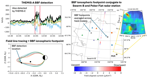
We select the BBF that occurred on 31 January 2018 for detailed analysis of its coupled FAC system and potential ionospheric effects. This BBF has its magnetic footpoint in north-west Alaska and is conjugate with Swarm-B and the PKR radar station. The triple conjugation was identified from the THEMIS-A BBF detection: THEMIS-E also observed the BBF but its magnetic footpoint was slightly too far from PKR to be automatically identified as a triple conjunction. THEMIS-D was within the magnetic lobe during this event and therefore was not located such that it could observe a BBF. Key details related to the timing and location of the THEMIS BBF detection are provided in Table 1. All times in this manuscript are provided in UTC.

Figure 1Key solar wind/IMF driving conditions and local geomagnetic activity during the 31 January 2018 BBF. The vertical red lines show the BBF start and end times. Subplots (a–c) show the IMF magnitude and components in GSE, solar wind velocity and dynamic pressure, respectively. Subplot (d) shows the local auroral indices that is calculated from local magnetometer stations, and subplot (e) shows the variation in the north/south component of the magnetic field (ΔBN) measured by these local stations. The ΔBN observations from different magnetometers are offset for clarity and arranged with decreasing geographic latitude from top to bottom; the black bar shows ΔB = 500 nT. Times are in UTC.
The 31 January 2018, BBF occurred during the recovery phase of a relatively weak substorm that occurred during fairly steady driving solar wind conditions. The driving solar wind/IMF conditions and local geomagnetic activity during this event is shown in Fig. 1. Figure 1a–c show the IMF magnitude and components in geocentric solar ecliptic (GSE) coordinates, solar wind velocity and solar wind dynamic pressure, with all data time-shifted to the bowshock nose and vertical red lines showing the start and end times of the BBF detection. Ground-based Alaskan magnetometer stations are used to calculated the local auroral indices, which are shown in Fig. 1d. Subplot e shows the magnetogram of these Alaskan magnetometers, showing the north/south magnetic field (minus the daily baseline) with an arbitrary, constant offset between the observations from different stations. Figure B1 provides the solar wind driving conditions and global geomagnetic and auroral indices over a longer time period for further context of this event. The driving solar wind conditions were overall quiet prior to the BBF observation; the solar wind velocity and IMF were near-constant with average vx = −336 km s−1 and = 3.5 nT throughout 30 January. A small magnetic cloud impacted the bowshock around 6 on 31 January, increasing to ∼ 8 nT. The magnetic cloud was originally dominated by the southward Bz, but rotated to become dominated by −By from ∼ 9 onward. There was a small (∼ 2 nPa) increase in the dynamic pressure during the −Bz period of the magnetic cloud, peaking at ∼ 4 nPa and then returning to nominal levels during the −By phase of the magnetic cloud. The southern Bz and slightly increased dynamic pressure is conducive to enhanced dayside magnetopause reconnection (Shue et al., 1998) and drove a weak substorm, with AE peaking at 326 nT at 09:59 on 31 January. There was a second, weaker peak in the auroral activity that began around 13 (shown by the auroral indices in Fig. B1d); the global AE peaked at 182 nT during this second substorm and the local AE (Fig. 1d) peaked at 409 nT over the same timeperiod.
Magnetic disturbances were observed by Alaskan magnetometer stations throughout the secondary substorm shown by the global auroral indices (Fig. B1d). The greatest changes in magnetic field were observed by the T41, CMO and EAG stations, which are at geographic latitudes ranging from 64.8–67.0°N, with the greatest ΔBN occurring at approximately 13:20 (all times are provided in UTC for the remainder of the article). There was significant spatial variation in the magnetic field changes observed by the ground based magnetometers: the FYU station, which is between T41 and the CMO/EAG stations, observed a smaller change in ΔBN that began approximately 15 min later than the ΔBN changes observed by T41, CMO and EAG. Furthermore, the T55 station at 60.5° N latitude did not observe any substantial magnetic field changes over the timeperiod plotted in Fig. 1. The magnetic field changes observed by these local magnetometer stations corresponds almost entirely to an enhancement of the westward electrojet, reflected in the enhancement of local AL while the local AU remains near-zero (Fig. 1d). The THEMIS BBF detections occurred during the recovery phase of this second peak in substorm activity, after the local minimum in ΔBN observed by the ground magnetometers (and therefore also after the peak in local auroral indices).

Figure 2THEMIS ion velocity observations and ion beta during the BBF detection. The dashed line in subplot d shows when βi=0.5. The vertical lines in subplots (a) and (b) show the start and end times of the BBF detected by THEMIS-A and -E, respectively. Times are in UTC.

Figure 3Magnetic field line tracing and footpoints of the 31 January 2018 BBF. Subplots (a) and (b) show the magnetic field line tracing from the THEMIS-A and -E locations during the BBF detections, and subplot (c) shows the location of the magnetic footpoints in geographic coordinates. In subplot (a) and (b), the locations of the three THEMIS satellites are shown by the black markers. In each subplot, the marker shape corresponds to the THEMIS satellite and the colour corresponds to the magnetic field model. The centroid footpoints in subplot (c) are grey. The Swarm-B overpass is also shown in subplot (c), with the colour corresponding to the field aligned current. The timestamps indicate when Swarm-B was at a given location. The location of the PKR radar station is shown by the gold star, while the spatial coverage of plasma velocity vectors derived from PKR data (plotted in Fig. 5) is indicated by the yellow box. Note that subplot (c) is in geographic coordinates and Fig. 5 is in magnetic coordinates, so the PKR data coverage visually differs in these two figures. Times are in UTC.
4.2 THEMIS observations
The THEMIS observations of the BBF are shown in Fig. 2. Figure 2a–c show the ion velocity observations for each satellite, with the vertical lines in subplots a and b showing the start and end times of the THEMIS-A and -E BBF detections, respectively. Figure 2d shows the ion beta (βi) from each THEMIS satellite during the event to contextualise the velocity data. There is a significant increase in βi around the BBF start times identified by George et al. (2026b), which indicates that the satellites entered the plasma sheet around the time of the BBF detection. We therefore refined the BBF start and end times by additionally requiring that βi>0.5 throughout the BBF, in addition to the identification criteria of George et al. (2026b). The BBF start and end times are therefore 13:44.38–13:47.36 (THEMIS-A) and 13:43.17–13:44.44 (THEMIS-E), modified from the George et al. (2026b) timings of 13:44.16–13:47.41 (THEMIS-A) and 13:40.13–13:46.45 (THEMIS-E). We use the refined BBF timing throughout this manuscript, including in Table 1. THEMIS-A and -E were located at (−10.4, −7.8, −2.2) RE and (−10.2, −5.9, −2.3) RE in GSM coordinates, respectively at the midpoint time of the BBF detection, which corresponds to a magnetic local time (MLT) of 2.5 and 2.0, respectively: in the postmidnight sector of the magnetotail. BBFs generally occur within ± 3 h of MLT around midnight with higher occurrence rate in the premidnight sector (Lanabere et al., 2025), which is consistent with magnetic reconnection site in the magnetotail having the highest occurrence rate in the premidnight sector but also sometimes occurring in the postmidnight sector (Nagai et al., 2023). The BBF analysed in this study is therefore within the typical statistical spatial distribution of BBFs, despite being further towards dawn than the majority of BBFs tend to occur.
The magnetic field line tracing from the locations of the THEMIS BBF detections and corresponding magnetic footpoints are shown in Fig. 3, which map to north-west Alaska. The location of the THEMIS-A, D, E satellites in Fig. 3a and b and their magnetic footpoints in Fig. 3c are shown by circles, squares and triangles, respectively. The magnetic field lines and footpoints obtained from different magnetic field models are shown in purple (T89), blue (T96), green (T01) and orange (T04). The centroid magnetic footpoints in Fig. 3c are shown in grey. The footpoints and field lines are shown at the midpoint time of the BBF detections, and we note that the field line tracing/footpoint determination was only performed for THEMIS-A and E since THEMIS-D did not observe the BBF. The magnetic footpoints of THEMIS-A are located eastward of the THEMIS-E footpoints and westward of PKR, which is shown by the gold star. The spatial coverage of the ionospheric plasma velocity vectors derived from PFISR data (described in Sect. 4.4) is shown by the yellow box. The location of Swarm-B is also shown in Fig. 3c with the colour scheme corresponding to FAC observations: negative FAC values (blue) correspond to an upward current and positive FAC values (red) correspond to a downward current. Swarm-B was initially located near the equator and travelled northward over Alaska: it was conjunctive with PKR at 13:53.15–13:53.55, and selected times are displayed to show when Swarm-B was in a given location. The Swarm-B trajectory was such that it traveled between the centroid magnetic footpoints obtained from the THEMIS-A and -E BBF detections.
The magnetic footpoints of the BBF are spread over a relatively broad area. The average distance between the centroid footpoints from THEMIS-A and -E for times where BBF observations are simultaneously available is 328 km. The ionospheric spatial coverage corresponding to the BBF observation can be estimated by treating the coupled BBF-ionosphere system as a single flux tube (as in the Chen and Wolf, 1993, model) and applying the conservation of magnetic flux as A1B1=A2B2. In this expression, A1 is the area of the BBF in the magnetotail, B1 is the magnetic field through the BBF (assumed to be purely in the z direction), A2 is the area of the BBF's ionospheric footpoint and B2 is the magnetic field through the ionospheric footpoint. THEMIS-A and -E were 1.87 RE apart in the Y direction at the time that they simultaneously observed the BBF. The minimum radius of the BBF would then be 0.935 RE, corresponding to the two THEMIS satellites being located on opposite edges of the BBF when they observe the BBF. The mean Bz observed by the two THEMIS satellites was 12.6 nT over the BBF duration, and the radial component of the dipole magnetic field at the locations of the centroid footpoints at 110 km altitude was 5.6 × 10⁴ nT. This corresponds to an ionospheric footprint size with radius of 90 km. We note that this is the lower bound on the ionospheric spatial scale: if we assume a BBF diameter of 3 RE instead of 1.87 RE, which is the statistical upper limit on the Y-length of BBFs (Sergeev et al., 1996), the corresponding ionospheric footpoint size is then 143 km. Both of these ionospheric footpoint size estimates are significantly smaller than the 328 km distance between the THEMIS-A and -E centroid footpoints. Furthermore, there is also a difference between the footpoint locations obtained from different models for the same THEMIS BBF observation. The THEMIS-A footpoints from different magnetic field models range from 68 km apart (time-averaged distance between footpoints obtained with the T96 and T04 models) to 288 km apart (distance between T01 and T04 footpoints), while the spread in THEMIS-E footpoints ranges from 76 km (distance between T96 and T04 footpoints) to 292 km (distance between T01 and T04 footpoints). There was also some temporal variation in the location of the centroid footpoint; the centroid BBF footpoint of the THEMIS-A (-E) traveled 43 km (20 km) over the duration of the BBF, which is minor compared to the differences in footpoint location obtained by different magnetic field models. The broad spread in magnetic footpoint locations when computed according to different magnetic field models or from BBF observations by the different THEMIS satellites is likely because the magnetic field models do not explicitly include BBFs, which likely decreases their accuracy when performing magnetic field line tracing of BBFs. However, since the collection of magnetic footpoints obtained by the different magnetic field models and THEMIS observations all map to north-west Alaska, we expect that the true ionospheric footprint of this BBF would indeed be within this region and therefore conjugate to PKR and Swarm-B.
An important factor when considering the ionospheric response to BBFs is the propagation time of the FAC from the BBFs location in the magnetotail to the ionosphere. We estimate this as the time for a signal that is traveling at the Alfven velocity (vA) to travel along the magnetic field line from the BBF location to the ionosphere. We calculate the length of the magnetic field lines obtained from each magnetic field model at one-minute time resolution throughout the THEMIS-A and -E BBF detections, and extract the magnetic field magnitude at each step along the field line. We then take a constant plasma density of ni=ne = 0.1 cm−3 along the field line (Haaland et al., 2017) to calculate the vA along that field line. The propagation time is then calculated as the mean time taken to travel at vA along the magnetic field lines, averaging across both time and magnetic field models. The minimum propagation time for a signal to travel from the BBF observed by THEMIS-A (-E) to the ionosphere obtained with this approach is 46 s (43 s). We emphasise that this is the minimum time between the BBF detection and the onset of any possible ionospheric effects at the ionospheric footpoint of the BBF, as it is possible that the FAC signal may travel slower than vA. Furthermore, the assumption of constant density along the field line does not account for increased density near the Earth due to ionospheric outflow, which would decrease the Alfven velocity and therefore increase the time taken to propagate along the field line. Inaccuracies in the magnetic field model would also lead to inaccuracies in this time delay estimation. However, these results indicate that the FAC associated with a BBF can reach the ionosphere (and therefore begin driving localised ionospheric dynamics) in timescales on the order of a minute from the BBFs detection in the magnetosphere.
4.3 Swarm observations
We evaluate the FAC signatures observed by Swarm-B during its overpass of the BBF magnetic footpoint. The multi-scale MVA (MS-MVA) analysis of the Swarm-B observations are shown in Fig. 4, which shows signatures consistent with BBF FAC at 13:54 and 13:55:30. Swarm-B was in the vicinity of the BBF magnetic footpoints (latitude ∼ 67°) at 13:54, while the 13:55:30 signature occurred when Swarm-B was significantly further poleward (latitude ∼ 73°). At these two times, the poleward component of the perturbation magnetic field (Bx) undergoes significant variation, and the FAC density rapidly fluctuates and reaches magnitudes of ≥ 5 µA m−2. The ratio between the maximum and intermediate eigenvalues is low (Fig. 4c), which indicates low planarity, and the inclination with respect to the East is high (Fig. 4f), consistent with the expected BBF FAC signature. The signatures in the eigenvalue ratio and inclination are highly temporally localised: the ∼ 13:54 signature has duration of ∼ 10's of seconds at window size below ∼ 10 s. Furthermore, the derivatives of the maximum and intermediate eigenvalues (Fig. 4d and e) maximize at window size of ∼ 10 s at 13:54, indicating comparable respective scales of some 100 km (Bunescu et al., 2015, 2019; Bunescu, 2024), once again consistent with the FAC system expected near the BBF footprint. The 13:54 FAC signatures are observed by Swarm-B approximately seven minutes after the end of the THEMIS-A BBF detection, which is several minutes longer than the estimated propagation time of the BBF-associated FAC from the magnetotail to the ionosphere. It is possible that the true propagation time of the FAC may be longer than our estimate, or that the FAC signatures persist for some time after the BBF has propagated Earthward. This FAC signature may also be associated with an ion flow burst that was observed by THEMIS-A shortly before 13:55 (see Fig. 2a): the velocity magnitude of this ion flow burst was too low to be classified as a BBF according to the George et al. (2026b) criteria, but it may have been sufficiently fast to support a FAC that coupled to the ionosphere to then be detected by Swarm during the overpass.

Figure 4Subplot a shows components of high-resolution (50 Hz) magnetic field perturbation in the NEC frame. Subplot (b) shows FAC density from low-resolution (1 Hz) data (blue) and from 20 s low-pass filtered data (orange). Subplot (c) shows the ratio of MVA eigenvalues (maximum/intermediate) at different scales, indicated on the y axes in seconds along satellite track. Subplot (d) (e) shows the derivative of the maximum (intermediate) eigenvalue with respect to the scale. Subplot(f) shows the current structure orientation with respect to the East direction in NEC. When performing MVA, we constrained the analysis to the plane perpendicular to the local magnetic field direction, which makes the third (minimum) eigenvalue always zero. Times are in UTC.
4.4 Poker Flat observations
We evaluate the ionospheric response to the BBF through analysis of the PKR observations. Figure 5 shows the plasma flow vectors, estimated from PFISR LoS data using the method by Tesfaw et al. (2025), overlaid against the PKR ASI observations mapped to 110 km altitude. The panels show nine subsequent time steps of the 1 min PFISR data around the THEMIS BBF detection time, with the ASI data averaged to the same time resolution in magnetic (aacgm_v2) coordinates. Figure B2 in the Appendix shows nine more time steps covering the Swarm-B overpass. The location of the THEMIS-A centroid magnetic footpoint is highlighted in Fig. 5, while the THEMIS-E centroid footpoint and trajectory of Swarm-B are both outside (westward) of the plotted area. The plasma convection (black arrows) is mostly eastward, as expected in the post-midnight sector, but in several panels superimposed vortex-like structures and other variations in the flow direction can be observed. In general, the largest plasma velocities are seen in the darker areas (blue colors), while the plasma flow is generally suppressed inside the brighter auroral structures.

Figure 5Plasma velocity vectors and 557.7 nm auroral emissions (in arbitrary units) around THEMIS BBF detection time. Plasma velocity vectors fitted to line-of-sight velocities measured with PFISR at selected grid points (black dots) are shown by lines, and emissions intensities from an ASI are shown by the colored background with red (blue) corresponding to the highest (lowest) intensity emissions. The ASI data are mapped to magnetic coordinates assuming 110 km emission altitude. Locations of centroid THEMIS-A footpoint and the Poker Flat radar site are shown by white circles: the centroid THEMIS-E footpoint is further west than the plotted area. Time stamps in each panel correspond to the mid-point of the 1 min integration period.
Auroral activity occurs throughout the time period plotted in Fig. 5, as is consistent with a substorm recovery phase. This auroral activity consists of patches of pulsating aurora and several bright, structured auroral features poleward of the pulsating aurora. In Fig. 5b–f, a transient auroral brightening develops around magnetic latitude of 71°, near the north Alaskan coastline. This auroral feature is oriented in the east-west direction, consistent with simulations of auroral streamers driven by BBFs (Workayehu et al., 2025), and the location of peak intensity moves westward before the auroral feature disappears. We note that the real shape of the auroral feature may be distorted due to the low elevation - for example a narrow arc covering a large altitude range could be seen as an latitudinally extended feature on the map. This auroral feature began before the THEMIS BBF detection and maps poleward of the THEMIS magnetic footpoints, so it is possible that this may be an auroral streamer that was driven by the BBF when it was located further away in the magnetotail, before it encountered the THEMIS satellites. The THEMIS velocity observations (Fig. 2) are predominantly in the −vy direction, which would correspond to eastward motion of the BBFs ionospheric footprint. We interpret this as the BBF's dominant motion being primarily in the +vy (westward) direction at the time of the auroral streamer, with the BBF then twisting to have the −vy (eastward) motion dominate by the time of the THEMIS observation. This is consistent with simulation studies of BBF propagation in the magnetotail (e.g. Birn et al., 2011) that demonstrate that BBFs can have significant and time-varying propagation in the y direction as they move Earthward and do not necessarily propagate directly radially inward throughout their lifetime. This interpretation of strong and time-varying vy over the lifetime of the BBF is further supported by the THEMIS-A velocity observations throughout the BBF (Fig. 2. THEMIS-A observed significantly negative vy (eastward) for the first ∼ of the BBF and then detected significantly positive vy (westward) ion velocity for the remainder of the BBF detection, demonstrating that the BBF propagation direction in Y did indeed vary as it propagated Earthward.

Figure 6Plasma parameters from PFISR beam number 2, which was pointed northwest with azimuth angle −16.2° and elevation 58.7°. Electron density (panel a), electron temperature (b), ion temperature (c), and line-of-sight plasma bulk velocity (d, positive away from the radar). Altitudes are shown on the left and magnetic latitudes on the right. The vertical lines show the BBF start and end times.
Another auroral feature occurs near at magnetic latitude around 66–67°, which became a distinct feature at approximately 13:30 and therefore is present throughout the time period plotted in Figs. 5 and B2. This feature is initially (in Fig. 5a) westward of the PFISR field-of-view (FoV) and propagates eastward over time: it is at the center of the PFISR FoV in Fig. 5i and continues eastward throughout the timeperiod plotted in Fig. B2. Motion of this auroral feature is associated with changes in the plasma flow direction and speed: the flow speed is clearly suppressed by the precipitation-enhanced conductivity when this auroral structure intersects the PFISR FoV (Fig. B2h and i).
Counter-clockwise plasma flow vortices occur in Fig. B2d, f, and i, which are associated with diverging electric fields and therefore correspond to downward FACs, as can be seen by considering the E-cross-B drift and ionospheric Ohm's law in the Northern Hemisphere. These counter-clockwise flow vortices associated with downward FAC have previously been observed by e.g. Munsami et al. (2002). These flow vortices are centered on areas of weaker auroral emissions. Aurora are generated by upward FAC (precipitating electrons) while the downward FAC is carried by upward flowing electrons, so the decrease in auroral activity in the vicinity of these plasma vortices is consistent with the downward FAC. These downward FAC signatures match the expected orientation of the FAC on the eastern edge of the BBF, and we therefore expect changes to the ionospheric plasma driven by the BBF to occur westward of these FAC signatures present in the PFISR data. Due to limited FoV of the radar, it is possible that the full ionospheric response to the BBF are not seen in the PFISR data. This downward FAC signature additionally validates that the magnetic footpoint of the BBF does indeed map to northern Alaska and to the west of the PKR radar station, consistent with the magnetic field mapping from the T89, T96, T01 and T04 models.
The ionospheric plasma parameters measured by a selected PFISR beam are shown in Fig. 6 as a function of time and altitude (left axis)/magnetic latitude (right axis). We select a beam oriented in north-west direction – pointing towards the expected location of the BBF's ionospheric footprint – at 58.7° elevation. Figure 6 shows the electron density (Ne), electron temperature (Te), ion temperature (Ti) and the line of sight (LoS) ion speed (, positive away from the radar) during a four hour period around the BBF. The start and end times of the BBF are shown by the vertical lines. The substorm growth phase, onset and expansion phase are clearly visible beginning around 13 in the Ne, Ti and panels, which corresponds to the time of local ground-based magnetic field disturbances (see Fig. 1e). As the growth phase arcs move southward of the radar (not shown), a temporary gap in the Ne is seen between 12:45–13:00 at altitudes below 150 km, with a corresponding increase in Ti caused by the enhanced plasma velocity. At approximately 13:02–13:05, the expansion phase aurora (not shown) briefly fills the PFISR beam FoV and enhances Ne and drives a reversal of the . This is quickly followed by another reversal of around 13:10 UT, which is associated with a counter-clockwise plasma flow vortex located northward of a bright auroral arc. The enhanced plasma convection increases the ion temperature. Activity continues throughout the substorm recovery phase, including during the BBF. There is a decrease in Ne at altitude of 150–200 km and reversal of seen during the BBF observation (marked by vertical lines), which are associated with the movement of auroral features across the radar beam and the appearance of vortex-like structures in the plasma velocity, as discussed above in connection to Fig. 5. This auroral structure was present for approximately 10–15 min before the BBF was detected in the magnetotail: the BBF may have been present deeper in the magnetotail prior to being detected, but its magnetic footpoint would have been significantly poleward of this auroral structure if it was present ∼ 10 min prior to the THEMIS detection. Therefore, this auroral structure is not driven by this BBF but is rather a manifestation of the broader magnetosphere–ionosphere coupling during the substorm. It is therefore likely that these ionospheric changes observed by PFISR at the time of the BBF detection are associated with the overall substorm dynamics and cannot be specifically attributed to the BBF itself.
BBFs are a key contributor to mass and energy flow from the magnetotail towards the Earth (Angelopoulos et al., 1994) and can contribute up to 10 % of the total energy deposited into the ionosphere during substorms (Ohtani, 2019). The FAC associated with a BBF are a key coupling mechanism between the BBF and the ionosphere. Upward oriented FAC corresponding to downward precipitating electrons, which can drive auroral streamers. The Earthward motion of the BBF corresponds to equatorward propagation of the ionospheric plasma that is coupled to that BBF, so BBFs can also drive equatorward plasma flows at their ionospheric footpoints. The precipitating electrons and ionospheric portion of the FAC system are associated with further localised changes to the ionospheric plasma, such as conductivity changes (Workayehu et al., 2025) or variation in the ionospheric temperature and density (Aikio et al., 2018).
In this study, we have evaluated triple-conjunctive observations of a BBF in the magnetotail, the FAC that may be associated with that BBF in low Earth orbit, and the ionospheric plasma dynamics in the vicinity of the BBF's magnetic footpoint. We identified these conjunctions between THEMIS and MMS BBF detections in the magnetotail, Swarm FAC measurements, and operating ground-based radar stations. A total of 11 086 BBFs were evaluated, from which we identify 13 events that satisfy our conjunction criteria: these triple-conjunctions (which correspond to 11 unique BBFs) are provided in Appendix A. We select the BBF that occurred on 31 January 2018, for detailed evaluation of the coupled BBF-FAC-ionosphere system during this event. This BBF occurred during a weak substorm and steady driving solar wind conditions, and the BBF was observed by two THEMIS satellites in the postmidnight sector of the magnetotail. The magnetic footpoints of the BBF observations were located in north-west Alaska, which was conjugate with the Swarm-B overpass and the PKR radar station. This analysis represents the first time that the coupled BBF-FAC-ionosphere system has been analysed during a single, isolated BBF using ionospheric radar observations that are immediately local to magnetic footpoint of the BBF.
Swarm-B detected FAC signatures that are characteristic of the FAC driven by BBFs. These FAC signatures include significant variations in the poleward component of the magnetic field perturbations and elevated current density, which occur on ∼ 100 km spatial scale with a low planarity and high inclination in the east-west direction. Swarm-B was located such that it passed between the two magnetic footpoints corresponding to the BBF detections by the two THEMIS satellites, although the overpass occurred minutes later than the estimated propagation time for a signal to propagate along the magnetic field line from the BBF's observed location within the magnetotail to the ionosphere. As a result, it is not completely clear whether these FAC signatures were associated with this specific BBF or if they correspond to a second flow burst observed by THEMIS a few minutes later that did not satisfy the velocity criteria to be identified as a BBF but may still have been fast enough to support a FAC system.
FAC signatures were also present in the radar observations, characterised by counter-clockwise plasma flow vortices that correspond to the downward component of the FAC system, as in e.g. Munsami et al. (2002). The downward FAC is established on the dawnside (eastward) edge of the BBF (Nakamura et al., 2001b; Liu et al., 2015), so these ionospheric observations are consistent with the majority of the BBF's ionospheric impact occurring westward of the PKR station. Indeed, the magnetic field mapping of the THEMIS BBF detections located the magnetic footpoints north-west of PKR. The radar beam observations to the north-west show changes in the ionospheric density, temperature and velocity throughout the weak substorm that this BBF occurred in. A velocity flow reversal was observed during and shortly after the BBF observation by THEMIS. At the same time, a plasma density decrease is observed at 66.0–66.5 Mlat (150–200 km altitudes), while a density increase is seen around 67 ML at (250–300 km). The changes in ionospheric plasma parameters around the BBF observation time were concurrent with an auroral structure moving into the PKR field of view: this auroral structure was not associated with the BBF as it was present for approximately 10–15 min before the BBF detection. Therefore, ionospheric dynamics observed at the time of the BBF detection seem to be associated with the broader substorm dynamics and cannot be specifically attributed to the ionospheric impacts of this BBF. However, another narrow, transient auroral structure was observed by the PKR ASI which does seem to be associated with the BBF, similarly to the auroral signatures of BBFs in e.g. Nakamura et al. (2001b). This auroral structure occurred further northward than the BBF magnetic footpoints and began several minutes before the BBF was detected by THEMIS, which is consistent with the BBF driving this aurora when it was more distant in the magnetotail and therefore mapping to higher latitudes.
Bursty bulk flows (BBFs) are mesoscale magnetotail structures that are ejected from magnetic reconnection sites and are characterised by fast plasma flows: they are responsible for the majority of transport of mass and energy from the magnetotail towards the Earth. BBFs couple to the ionosphere via field aligned currents (FAC) and contribute up to 10 % of the energy deposited into the ionosphere during substorms. In this study, we identified triple conjunctive observations of different aspects of the coupled BBF-FAC-ionosphere system. We evaluated over 11 000 BBFs observed by MMS and THEMIS and identified 13 triple-conjunctions (11 unique BBFs) that are conjugate with the Swarm constellation that measures FAC in low Earth orbit and ground-based radar stations that measure the local ionospheric plasma. We then performed detailed analysis of one of these events that occurred during a weak substorm, and identified multiple FAC structures that may be associated with this BBF. Variation in the ionospheric plasma occurred during and after the BBF observation, although isolating the ionospheric dynamics that are driven by BBFs from those related to the overall substorm dynamics remains an open question. Cross-region coupling is an essential component of substorm activity, particularly between the ionosphere and magnetotail, and further research is needed to fully evaluate the role that mesoscale structures such as BBFs play in energy and mass transport across different regions of geospace during substorms. Cross-region coupling has been highlighted as a science focus by the mission concepts Plasma Observatory (ESA) and Links (NASA), which would both observe the magnetotail and nightside transition region. Coordinated observations between these future (and existing) magnetospheric missions and ground-based and/or low Earth orbiting satellites that can observe the ionospheric signatures of BBFs will enable further evaluation of the role of these mesoscale structures in magnetotail-ionosphere coupling.
Table A1 summarises key details on all triple conjunctions identified in this study between a BBF detection in the magnetotail by MMS or THEMIS, a Swarm satellite and an operating radar station. The BBF detection location is in GSM coordinates and is provided at the midpoint time of the BBF detection according to the Richard et al. (2022) and George et al. (2026b) identification criteria. The distance from the BBF footpoint to the radar is specifically the minimum distance between the centroid footpoint and radar station over the duration of the BBF. The time of the Swarm/radar conjunction is defined as the time period where Swarm was within 400 km of a given radar station.
Table A1Triple conjunctions between BBF detections in the magnetotail, Swarm and an operating radar station.

Figure B1 shows the solar wind/IMF driving conditions and geomagnetic indices over a broader time period than Fig. 1 to further contextualise the conditions in which the 31 January 2018 BBF occurs. The time of the BBF detection by THEMIS is indicated by the vertical red line. Figure B2 shows the PKR observations in the same format as Fig. 5 but for a slightly later time period that encompasses the Swarm-B overpass.

Figure B1Solar wind and geomagnetic conditions during the BBF, showing a greater time period than Fig. 1 for additional context. The vertical red line highlights the time of the BBF. In subplot (e), the Hp30 data corresponds to the left axis and Dst corresponds to the right axis, with the dashed grey line showing Dst of 0 nT. Times are in UTC.

Figure B2Plasma velocity vectors and 557.7 nm auroral emissions around the Swarm overpass time. Plasma velocity vectors fitted to line-of-sight velocities measured with PFISR at selected grid points (black dots) are shown by lines, and emissions intensities from an ASI are shown by the colored background. The ASI data are mapped to magnetic (aacgm_v2) coordinates assuming 110 km emission altitude. Locations of THEMIS-A footpoint and the Poker Flat radar site are shown by white circles.
All data analysed in this study are publicly available. Conjunctions between the magnetic footpoint of a BBF and a radar station, and between a Swarm satellite and a radar station are provided at https://doi.org/10.5281/zenodo.20448704 (George et al., 2026a). The THEMIS data is available at https://themis.ssl.berkeley.edu/data/themis/ (last access: 29 May 2026). The PKR all-sky camera data are available at http://optics.gi.alaska.edu/optics/?q=archive (last access: 29 May 2026) and the calibration data with azimuth/elevation information at https://optics.gi.alaska.edu/amisr_archive/Cal_data/PKR/DASC/azel/ (last access: 29 May 2026). The PFISR data can be accessed from the CEDAR Madrigal database at https://w3id.org/cedar?experiment_list=experiments3/2018/pfa/26jan18f&file_list=pfa180126.006.hdf5 (last access: 29 May 2026). Swarm data is available at https://earth.esa.int/eogateway/missions/swarm/data (last access: 29 May 2026). SuperMag data is available at https://supermag.jhuapl.edu/mag/ (last access: 29 May 2026) and the solar wind data are accessible at https://cdaweb.gsfc.nasa.gov/ (last access: 29 May 2026). Dst indices and solar wind/IMF parameters that are inputs to these magnetospheric models are obtained from the OMNI CDAWeb https://cdaweb.gsfc.nasa.gov/ (last access: 29 May 2026), and the Hp30 indices are obtained from https://www.gfz.de/en/hpo-index (last access: 29 May 2026).
The contact author has declared that none of the authors has any competing interests.
Publisher's note: Copernicus Publications remains neutral with regard to jurisdictional claims made in the text, published maps, institutional affiliations, or any other geographical representation in this paper. The authors bear the ultimate responsibility for providing appropriate place names. Views expressed in the text are those of the authors and do not necessarily reflect the views of the publisher.
HG led the analysis of the magnetospheric data, prepared the figures showing THEMIS and solar wind observations, and led the writing of the manuscript. AD, VL and SB contributed to the analysis of magnetospheric data and methodology development. IV and HT performed the PFISR analysis, and MM performed the ASI analysis and mapping. IV prepared the figures of PKR observations. HV and AA contributed to the analysis and interpretation of radar and aurora observations. OM and AB prepared the figure showing Swarm results and led the analysis of Swarm data. MS assisted in the interpretation of the auroral observations. All coauthors participated in discussion of the results and the preparation of the manuscript.
We thank Steve Morley for providing the QinDenton parameters used to perform the magnetic field line tracing with the T01 and T04 magnetic field models, Joachim Vogt for the efficient and handy implementation of the MS-MVA technique, and Asti Bhatt for support in PFISR data analysis. We acknowledge NASA contract NAS5-02099 and Vassilis Angelopoulos for use of data from the THEMIS Mission, specifically Charles Carlson and James McFadden for use of ESA data. We acknowledge ESA for the Swarm mission. AMISR facilities are operated and maintained for the US National Science Foundation (NSF) by SRI International under a cooperative agreement AGS-1840962. AMISR data are produced and made publicly available for scientific and academic research purposes under the same award. We gratefully acknowledge SuperMag and its collaborators for the ground magnetometer data (https://supermag.jhuapl.edu/info/?page=acknowledgement, last access: 29 May 2026), and the NASA/GSFC's Space Physics Data Facility's OMNIWeb service.
This work was supported by the ESA 4D ionosphere initiative through the ESA contract No. 383 4000143412/23/I-EB under a CCN between the FBURST and JOIN contracts. A.P.D. received financial support from the Swedish National Space Agency (grant 2020-00111). A.A. acknowledges support from the Research Council of Finland (RCF) projects SpaceResilience (grant no. 374100) and INTERSECT (grant no. 348782). H.V. acknowledges support from the RCF project AuroralJoule (grant no. 354521). I.V. acknowledges support from the Research Council of Finland project IONTRACE (grant no. 367883). A.B. and O.M. acknowledge support from the project MAGICS, ESA PRODEX contract 4000127660.
The publication of this article was funded by the Swedish Research Council, Forte, Formas, and Vinnova.
This paper was edited by Georgios Balasis and reviewed by Malcolm Dunlop and one anonymous referee.
Aikio, A. T., Vanhamäki, H., Workayehu, A. B., Virtanen, I. I., Kauristie, K., Juusola, L., Buchert, S., and Knudsen, D.: Swarm Satellite and EISCAT Radar Observations of a Plasma Flow Channel in the Auroral Oval Near Magnetic Midnight, J. Geophys. Res.-Space, 123, 5140–5158, https://doi.org/10.1029/2018JA025409, 2018. a, b
Akasofu, S.-I.: The development of the auroral substorm, Planet. Space Sci., 12, 273–282, https://doi.org/10.1016/0032-0633(64)90151-5, 1964. a
Akasofu, S.-I.: A new understanding of why the aurora has explosive characteristics, Mon. Not. R. Astron. Soc., 518, 3286–3300, https://doi.org/10.1093/mnras/stac3187, 2023. a, b
Angelopoulos, V., Kennel, C. F., Coroniti, F. V., Pellat, R., Kivelson, M. G., Walker, R. J., Russell, C. T., Baumjohann, W., Feldman, W. C., and Gosling, J. T.: Statistical characteristics of bursty bulk flow events, J. Geophys. Res.-Space, 99, 21257–21280, https://doi.org/10.1029/94JA01263, 1994. a, b
Angelopoulos, V., McFadden, J. P., Larson, D., Carlson, C. W., Mende, S. B., Frey, H., Phan, T., Sibeck, D. G., Glassmeier, K.-H., Auster, U., Donovan, E., Mann, I. R., Rae, I. J., Russell, C. T., Runov, A., Zhou, X.-Z., and Kepko, L.: Tail Reconnection Triggering Substorm Onset, Science, 321, 931–935, https://doi.org/10.1126/science.1160495, 2008a. a
Angelopoulos, V., Sibeck, D., Carlson, C. W., McFadden, J. P., Larson, D., Lin, R. P., Bonnell, J. W., Mozer, F. S., Ergun, R., Cully, C., Glassmeier, K. H., Auster, U., Roux, A., LeContel, O., Frey, S., Phan, T., Mende, S., Frey, H., Donovan, E., Russell, C. T., Strangeway, R., Liu, J., Mann, I., Rae, J., Raeder, J., Li, X., Liu, W., Singer, H. J., Sergeev, V. A., Apatenkov, S., Parks, G., Fillingim, M., and Sigwarth, J.: First Results from the THEMIS Mission, Space Sci. Rev., 141, 453–476, 2008b. a
Auster, H. U., Glassmeier, K. H., Magnes, W., Aydogar, O., Baumjohann, W., Constantinescu, D., Fischer, D., Fornacon, K. H., Georgescu, E., Harvey, P., Hillenmaier, O., Kroth, R., Ludlam, M., Narita, Y., Nakamura, R., Okrafka, K., Plaschke, F., Richter, I., Schwarzl, H., Stoll, B., Valavanoglou, A., and Wiedemann, M.: The THEMIS Fluxgate Magnetometer, Space Sci. Rev., 141, 235–264, 2008. a
Bhatt, A.: Data from the CEDAR Madrigal database, CEDAR Madrigal Database [data set], https://w3id.org/cedar?experiment_list=experiments3/2018/pfa/26jan18f&file_list=pfa180126.006.hdf5 (last access: 29 May 2026), 2018. a, b
Birn, J., Raeder, J., Wang, Y. L., Wolf, R. A., and Hesse, M.: On the propagation of bubbles in the geomagnetic tail, Ann. Geophys., 22, 1773–1786, https://doi.org/10.5194/angeo-22-1773-2004, 2004. a
Birn, J., Nakamura, R., Panov, E. V., and Hesse, M.: Bursty bulk flows and dipolarization in MHD simulations of magnetotail reconnection, J. Geophys. Res.-Space, 116, https://doi.org/10.1029/2010JA016083, 2011. a, b
Blagau, A. and Vogt, J.: SwarmFACE: a Python Package for Field-Aligned Currents Exploration with Swarm, Frontiers in Astronomy and Space Sciences, 9, 418, https://doi.org/10.3389/fspas.2022.1077845, 2023. a
Blinstrubas, G., English, A., Stuart, D. J., Hampton, D. L., Lamarche, L., Nishimura, Y., and Datta-Barua, S.: Comparative Hypothesis Testing of Auroral Ionospheric Layer Causing Global Navigation Satellite System Scintillation, Space Weather, 23, e2024SW004069, https://doi.org/10.1029/2024SW004069, 2025. a
Bunescu, C.: The Structure of Field-Aligned Current Systems as Inferred From the Multiscale Minimum Variance Analysis, Earth and Space Science, 11, e2024EA003708, https://doi.org/10.1029/2024EA003708, 2024. a, b
Bunescu, C., Marghitu, O., Constantinescu, D., Narita, Y., Vogt, J., and Blăgău, A.: Multiscale field-aligned current analyzer, J. Geophys. Res.-Space, 120, 9563–9577, https://doi.org/10.1002/2015JA021670, 2015. a, b
Bunescu, C., Vogt, J., Marghitu, O., and Blagau, A.: Multiscale estimation of the field-aligned current density, Ann. Geophys., 37, 347–373, https://doi.org/10.5194/angeo-37-347-2019, 2019. a, b
Chen, C. X. and Wolf, R. A.: Interpretation of high-speed flows in the plasma sheet, J. Geophys. Res.-Space, 98, 21409–21419, https://doi.org/10.1029/93JA02080, 1993. a, b
Fairfield, D. H., Tsyganenko, N. A., Usmanov, A. V., and Malkov, M. V.: A large magnetosphere magnetic field database, J. Geophys. Res.-Space, 99, 11319–11326, https://doi.org/10.1029/94JA00255, 1994. a
Friis-Christensen, E., Lühr, H., and Hulot, G.: Swarm: A constellation to study the Earth's magnetic field, Earth Planets Space, 58, 351-358, https://doi.org/10.1186/BF03351933, 2006. a
George, H., Dimmick, A., Lanabere, V., Vanhamäki, H., Virtanen, I., and Aikio, A.: Conjunctions: BBF-radar and Swarm-radar, Zenodo [data set], https://doi.org/10.5281/zenodo.20448704, 2026a. a, b
George, H., Ergun, R., Rogers, A., Genestreti, K., and Gabrielse, C.: Cross-tail extent of magnetotail reconnection from bursty bulk flow distribution, ESS Open Archive [preprint], https://doi.org/10.22541/essoar.15008751/v1, 2026b. a, b, c, d, e, f, g, h
Gjerloev, J. W.: A Global Ground-Based Magnetometer Initiative, Eos T. Am. Geophys. Un., 90, 230–231, https://doi.org/10.1029/2009EO270002, 2009. a
Gjerloev, J. W.: The SuperMAG data processing technique, J. Geophys. Res.-Space, 117, https://doi.org/10.1029/2012JA017683, 2012. a
Haaland, S., Lybekk, B., Maes, L., Laundal, K., Pedersen, A., Tenfjord, P., Ohma, A., Østgaard, N., Reistad, J., and Snekvik, K.: North-south asymmetries in cold plasma density in the magnetotail lobes: Cluster observations, J. Geophys. Res.-Space, 122, 136–149, https://doi.org/10.1002/2016JA023404, 2017. a
Heinselman, C. J. and Nicolls, M. J.: A Bayesian approach to electric field and E -region neutral wind estimation with the Poker Flat Advanced Modular Incoherent Scatter Radar, Radio Sci., 43, RS5013, https://doi.org/10.1029/2007rs003805, 2008. a, b
Juusola, L., Nakamura, R., Amm, O., and Kauristie, K.: Conjugate ionospheric equivalent currents during bursty bulk flows, J. Geophys. Res.-Space, 114, https://doi.org/10.1029/2008JA013908, 2009. a, b
Kloss, C., Finlay, C. C., Olsen, N., Tøffner-Clausen, L., Gillet, N., and Grayver, A.: The CHAOS-8 geomagnetic field model, Earth Planets Space, 78, 21, https://doi.org/10.1186/s40623-025-02352-0, 2026. a
Lanabere, V., Dimmock, A. P., Richard, L., Buchert, S., Khotyaintsev, Y. V., and Marghitu, O.: Variability in footpoint mapping of bursty bulk flows using Tsyganenko models: impact on swarm conjunctions, J. Space Weather Spac., 15, 41, https://doi.org/10.1051/swsc/2025035, 2025. a, b, c
Lanabere, V., Buchert, S., Blagau, A., George, H., Nanjo, S., Juusola, L., Dimmock, A. P., Wharton, S., Vanhamäki, H., Marghitu, O., Richard, L., Cai, L., Wallner, A. V. L., Kotova, D., Jin, Y., Hoppe, T., Carter, J. A., and Aikio, A.: Ionospheric currents and auroral signatures during successive earthward bursty bulk flows and dipolarization: a 7 December 2023 case study, Ann. Geophys., 44, 977–1001, https://doi.org/10.5194/angeo-44-977-2026 2026. a, b
Lin, R. L., Zhang, X. X., Liu, S. Q., Wang, Y. L., and Gong, J. C.: A three-dimensional asymmetric magnetopause model, J. Geophys. Res.-Space, 115, https://doi.org/10.1029/2009JA014235, 2010. a
Liu, J., Angelopoulos, V., Chu, X., Zhou, X.-Z., and Yue, C.: Substorm current wedge composition by wedgelets, Geophys. Res. Lett., 42, 1669–1676, https://doi.org/10.1002/2015GL063289, 2015. a, b
Lynch, K. A., Hampton, D. L., Zettergren, M., Bekkeng, T. A., Conde, M., Fernandes, P. A., Horak, P., Lessard, M., Miceli, R., Michell, R., Moen, J., Nicolls, M., Powell, S. P., and Samara, M.: MICA sounding rocket observations of conductivity-gradient-generated auroral ionospheric responses: Small-scale structure with large-scale drivers, J. Geophys. Res.-Space, 120, 9661–9682, https://doi.org/10.1002/2014JA020860, 2015. a
McFadden, J. P., Carlson, C. W., Larson, D., Ludlam, M., Abiad, R., Elliott, B., Turin, P., Marckwordt, M., and Angelopoulos, V.: The THEMIS ESA Plasma Instrument and In-flight Calibration, Space Sci. Rev., 141, 277–302, 2008. a
McPherron, R. L.: Magnetospheric substorms, Rev. Geophys., 17, 657–681, https://doi.org/10.1029/RG017i004p00657, 1979. a
McPherron, R. L.: Where and when does reconnection occur in the tail?, J. Geophys. Res.-Space, 121, 4607–4610, https://doi.org/10.1002/2015JA022258, 2016. a
Morley, S.: QinDenton, GitHub [code], https://github.com/drsteve/QinDenton/ (last access: 29 May 2026), 2017. a
Munsami, V., Pinnock, M., and Rodger, A. S.: HF radar observation of field-aligned currents associated with quiet time transient flow bursts in the magnetosphere, J. Geophys. Res.-Space, 107, SMP 8–1–SMP 8–10, https://doi.org/10.1029/2001JA000185, 2002. a, b, c
Nagai, T., Shinohara, I., Saito, Y., Ieda, A., and Nakamura, R.: Location and Timing of Magnetic Reconnections in Earth's Magnetotail: Accomplishments of the 29-Year Geotail Near-Earth Magnetotail Survey, J. Geophys. Res.-Space, 128, e2023JA032023, https://doi.org/10.1029/2023JA032023, 2023. a
Nakamura, R., Baumjohann, W., Schödel, R., Brittnacher, M., Sergeev, V. A., Kubyshkina, M., Mukai, T., and Liou, K.: Earthward flow bursts, auroral streamers, and small expansions, J. Geophys. Res.-Space, 106, 10791–10802, https://doi.org/10.1029/2000JA000306, 2001a. a
Nakamura, R., Baumjohann, W., Schödel, R., Brittnacher, M., Sergeev, V. A., Kubyshkina, M., Mukai, T., and Liou, K.: Earthward flow bursts, auroral streamers, and small expansions, J. Geophys. Res.-Space, 106, 10791–10802, https://doi.org/10.1029/2000JA000306, 2001b. a, b, c
Nicolls, M. J. and Heinselman, C. J.: Three-dimensional measurements of traveling ionospheric disturbances with the Poker Flat Incoherent Scatter Radar, Geophys. Res. Lett., 34, L21104, https://doi.org/10.1029/2007GL031506, 2007. a
Ohtani, S.: Substorm Energy Transport From the Magnetotail to the Nightside Ionosphere, J. Geophys. Res.-Space, 124, 8669–8684, https://doi.org/10.1029/2019JA026964, 2019. a, b
Ohtani, S.-i., Shay, M. A., and Mukai, T.: Temporal structure of the fast convective flow in the plasma sheet: Comparison between observations and two-fluid simulations, J. Geophys. Res.-Space, 109, https://doi.org/10.1029/2003JA010002, 2004. a
Pitkänen, T., Aikio, A. T., Amm, O., Kauristie, K., Nilsson, H., and Kaila, K. U.: EISCAT-Cluster observations of quiet-time near-Earth magnetotail fast flows and their signatures in the ionosphere, Ann. Geophys., 29, 299–319, https://doi.org/10.5194/angeo-29-299-2011, 2011. a, b, c
Qin, Z., Denton, R. E., Tsyganenko, N. A., and Wolf, S.: Solar wind parameters for magnetospheric magnetic field modeling, Space Weather, 5, https://doi.org/10.1029/2006SW000296, 2007. a
Richard, L., Khotyaintsev, Y. V., Graham, D. B., and Russell, C. T.: Are Dipolarization Fronts a Typical Feature of Magnetotail Plasma Jets Fronts?, Geophys. Res. Lett., 49, e2022GL101693, https://doi.org/10.1029/2022GL101693, 2022. a, b
Sergeev, V. A., Angelopoulos, V., Gosling, J. T., Cattell, C. A., and Russell, C. T.: Detection of localized, plasma-depleted flux tubes or bubbles in the midtail plasma sheet, J. Geophys. Res.-Space, 101, 10817–10826, https://doi.org/10.1029/96JA00460, 1996. a, b
Sergeev, V. A., Liou, K., Newell, P. T., Ohtani, S.-I., Hairston, M. R., and Rich, F.: Auroral streamers: characteristics of associated precipitation,convection and field-aligned currents, Ann. Geophys., 22, 537–548, https://doi.org/10.5194/angeo-22-537-2004, 2004. a
Shue, J.-H., Song, P., Russell, C. T., Steinberg, J. T., Chao, J. K., Zastenker, G., Vaisberg, O. L., Kokubun, S., Singer, H. J., Detman, T. R., and Kawano, H.: Magnetopause location under extreme solar wind conditions, J. Geophys. Res.-Space, 103, 17691–17700, https://doi.org/10.1029/98JA01103, 1998. a
Sonnerup, B. U. Ö. and Scheible, M.: Minimum and Maximum Variance Analysis, ISSI Scientific Reports Series, ESA/ISSI , 1, 185–220, 1998. a
Tesfaw, H. W., Vanhamäki, H., Virtanen, I., Hatch, S., Zettergren, M., and Laundal, K.: Modeling Regional Electric Field Using EISCAT3D Observations, J. Geophys. Res.-Space, 130, e2024JA033625, https://doi.org/10.1029/2024JA033625, 2025. a, b
Tian, S.: Geopack, Zenodo [code], https://doi.org/10.5281/zenodo.15110786, 2018. a
Tsyganenko, N. A.: A magnetospheric magnetic field model with a warped tail current sheet, Planet. Space Sci., 37, 5–20, https://doi.org/10.1016/0032-0633(89)90066-4, 1989. a
Tsyganenko, N. A.: Effects of the solar wind conditions in the global magnetospheric configurations as deduced from data-based field models (Invited), in: International Conference on Substorms, edited by Rolfe, E. J. and Kaldeich, B., vol. 389 of ESA Special Publication, p. 181, 1996ESASP.389..181T, 1996. a
Tsyganenko, N. A.: A model of the near magnetosphere with a dawn-dusk asymmetry 1. Mathematical structure, J. Space Weather Spac. 107, 1179, https://doi.org/10.1029/2001JA000219, 2002a. a
Tsyganenko, N. A.: A model of the near magnetosphere with a dawn-dusk asymmetry 2. Parameterization and fitting to observations, J. Space Weather Spac. 107, 1176, https://doi.org/10.1029/2001JA000220, 2002b. a, b
Tsyganenko, N. A. and Sitnov, M. I.: Modeling the dynamics of the inner magnetosphere during strong geomagnetic storms, J. Space Weather Spac. 110, A03208, https://doi.org/10.1029/2004JA010798, 2005. a
Wei, D., Dunlop, M. W., Yang, J., Dong, X., Yu, Y., and Wang, T.: Intense dB/dt Variations Driven by Near-Earth Bursty Bulk Flows (BBFs): A Case Study, Geophys. Res. Lett., 48, e2020GL091781, https://doi.org/10.1029/2020GL091781, 2021. a
Wiltberger, M., Merkin, V., Lyon, J. G., and Ohtani, S.: High-resolution global magnetohydrodynamic simulation of bursty bulk flows, J. Geophys. Res.-Space, 120, 4555–4566, https://doi.org/10.1002/2015JA021080, 2015. a
Workayehu, A., Palmroth, M., Grandin, M., Juusola, L., Alho, M., Zaitsev, I., Koikkalainen, V., Horaites, K., Pfau-Kempf, Y., Ganse, U., Battarbee, M., and Suni, J.: Ionospheric signatures of a Bursty Bulk Flow in the 6D Vlasiator simulation, Ann. Geophys., 43, 723–737, https://doi.org/10.5194/angeo-43-723-2025, 2025. a, b, c
Yamazaki, Y., Matzka, J., Stolle, C., Kervalishvili, G., Rauberg, J., Bronkalla, O., Morschhauser, A., Bruinsma, S., Shprits, Y. Y., and Jackson, D. R.: Geomagnetic Activity Index Hpo, Geophys. Res. Lett., 49, e2022GL098860, https://doi.org/10.1029/2022GL098860, 2022. a
Yang, Z., Zhang, B., Lotko, W., and Lei, J.: Global Evolution, Energetics, and Origins of Auroral Streamers, Geophys. Res. Lett., 52, e2025GL115681, https://doi.org/10.1029/2025GL115681, 2025. a
Yu, Y., Cao, J., Fu, H., Lu, H., and Yao, Z.: The effects of bursty bulk flows on global-scale current systems, J. Geophys. Res.-Space, 122, 6139–6149, https://doi.org/10.1002/2017JA024168, 2017. a