
the Creative Commons Attribution 4.0 License.
the Creative Commons Attribution 4.0 License.
 | 18 Nov 2026
Propagation of interplanetary (IP) shocks near the Earth

Yoshihiro Yokoyama
Tsubasa Kotani
Jürgen Matzka
Solar wind values monitored at the Sun–Earth L1 point have been used to estimate the Earth-arrival time of interplanetary (IP) shocks associated with coronal mass ejections (CMEs) and co-rotating interaction regions (CIRs). In standard estimates, including NASA/OMNI database, the radial propagation speed of the IP shock is assumed to be the same as the measured solar wind (proton) speed after the shock, although these speeds are known to be different in both the shock theory and CME observations. To diagnose the actual differences between these speeds, we statistically compared them using spacecraft data at L1. The propagation speed is obtained from the time-of-propagation between the IP shock passage at the L1 monitoring point and the geomagnetic sudden commencement (SC) at the Earth. As the L1 monitoring point, we use three locations: two are the spacecraft (SOHO and ACE) locations, and the other is the estimated IP shock passage point upstream of the Earth nearest to in Geocentric Solar Ecliptic (GSE) coordinate that is calculated from timings and locations of the IP shock passage at both spacecraft (we call the triangle method). In statistics, we limited to the IP shocks with a clear geomagnetic SC signature and with velocity profiles consistent between SOHO and ACE. During 1998–2022, 375 IP shocks satisfied such conditions. For the solar wind speed (VSW), the highest value during 15 min after the IP shock passage observed by the selected spacecraft (SOHO or ACE) was used. We found the following tendencies. (1) As expected from the shock theory, arrival time of the IP shock to the Earth (represented by the geomagnetic SC) is earlier than the predicted arrival time of the shocked solar wind by 0–8 min. (2) The speed difference between the shock propagation and VSW after the shock (highest value during 15 min) is about +7 % compared to SOHO observation and +10 % compared to ACE observation. (3) Tilt angle of the shock estimated by simple 1D shock model using velocity changes across the shock of ACE gives, although this method has large instrumental uncertainty, generally consistent values what is estimated by triangle method within the uncertainty.
- Article
(6639 KB) - Full-text XML
- BibTeX
- EndNote


In solar-terrestrial physics including the relevant magnetospheric physics and space weather predictions, upstream monitoring of the solar wind parameters such as the velocity, density, and the interplanetary magnetic field (IMF) is essential. The upstream measurements of these values have been continuously made by monitoring spacecraft at the Sun–Earth Lagrange L1 region for nearly three decades by Wind (Oglivie et al., 1995), SOHO (Ipavich et al., 1998) and ACE (McComas et al., 1998), and one decade by DSCOVR. With solar wind velocity and distance between these spacecraft and the Earth, one can roughly estimate the arrival time of the coronal mass ejection (CME) and other large changes in these parameters, such as interplanetary (IP) shocks and large IMF changes.
In these estimates of the arrival time, such as in the 1 min OMNI data at NASA Omniweb site (https://omniweb.gsfc.nasa.gov/, last access: 16 June 2026) in which the solar wind data is projected at the Earth's bow shock nose location, the earthward propagation speed of the CME and other IP shocks along the Geocentric Solar Ecliptic (GSE) coordinate −XGSE direction is normally assumed to be the same as the solar wind speed (anti-sunward proton speed) after the shock that is measured at L1 (King and Papitashvili, 2026). However, the propagation speed of the IP shocks is known to be different from the solar wind speed in both the shock theory and CME observations.
For observation near the Sun, the CME front identified by SOHO LASCO imager sometimes propagates at velocity >1000 km s−1, being much faster than the solar wind velocity measured at L1 (e.g., Manoharan et al., 2001; Yashiro et al., 2004; Tokumaru et al., 2006; Gonzalez-Esparza and Aguilar-Rodriguez, 2009; Gopalswamy et al., 2009). Although the CME propagation is decelerated while the solar wind is accelerated with distance from the Sun, the IP shocks propagate faster than the solar wind even near the Earth.
In 1D shock models, the conservation of the mass flux across the shock in the shock-rest frame (Rankine-Hugoniot relation) requires that the higher-density side (solar wind after the IP shock passage for forward shock) should have lower relative velocity to the shock. This condition can be achieved only if the shock speed is higher than the solar wind speed (see Fig. A1 in Appendix A for this textbook type relation).
Theoretically, the shock propagation speed should be able to be derived from the measured changes in velocity and density. However, the observation of density, particularly its large increase, is often erroneous right after the IP shocks, causing such a calculated result unreliable (cf. Sect. 2.2 and Appendix A2). This is one of the reasons why the solar wind speed is used for predicting the arrival time of the IP shocks at the Earth. Furthermore, the actual IP shocks are not as ideal as simple models (e.g., local inhomogeneity or wavy structures, which makes even the local shock normal direction different from the large-scale normal direction), and it is wise to avoid using local 1D model in automated prediction of the large-scale propagation.
The time difference comes also from obliquely directed shock front surface (“phase plane”) because the location of the monitor spacecraft (SOHO, ACE, and DSCOVR) is largely offset in the GSE Y–Z direction from the Sun–Earth line (Richardson and Paularena, 1998; Collier et al., 1998), at distances up to km for ACE (https://izw1.caltech.edu/ACE/ASC/DATA/browse-html/y_z_plot.gif, last access: 16 November 2026) and up to km for SOHO (https://soho.nascom.nasa.gov/about/orbit.html, last access: 16 November 2026) away from the Sun–Earth line in the huge L1 region. In such cases, the passage time of the IP shock at the same XGSE location as the monitoring spacecraft can be significantly earlier or later than those at the monitoring spacecraft, causing the estimation error in the predicted arrival time of the IP shock at the Earth. Fortunately, both SOHO and ACE take nearly symmetric orbits with respect to the Sun–Earth line (i.e., in the GSE Y–Z direction). Therefore, the statistical average of the actual arrival time is expected to converge to the expected arrival time, unlike the time difference coming from the difference in speeds.
Since the arrival time of the IP shocks to the Earth is one essential information in understanding the solar wind-magnetosphere interaction including the space weather prediction, it is quite important to examine the degree of difference between the radial propagation speed of IP shocks (particularly of CMEs) and the speed of the solar wind near the Earth. This type of difference has been reported for the transit time of the IMF changes (e.g., Collier et al., 1998; Milan et al., 2022), but less well studied for the IP shocks (e.g., Paularena et al., 1998, 1999). Particularly, no statistical study on the difference in the speed (between the IP shock propagation and solar wind) near the Earth was made, although the statistical study is mandatory from the above reasons.
The purpose of this paper is to statistically examine the velocity difference between the IP shock propagation and solar wind speed (accordingly, the difference in the arrival time to the Earth) using the solar wind data from the L1 monitoring spacecraft (both SOHO and ACE) and the geomagnetic data. From solar wind data, we obtained the timing of the IP shock passage (Tsoho for SOHO and Tace for ACE) at the spacecraft location and the solar wind speed (VSW) after the IP shock passage, whereas we used geomagnetic data to determine the timing of the geomagnetic sudden commencement (SC) as the proxy of the arrival time of the IP shock to the Earth (TSC). Decades of L1 monitoring by SOHO (since 1996) and ACE (since 1997) allows us to take statistics on the difference in speed between the IP shock propagation and the solar wind, using a sufficient number of IP shocks that are identified in both spacecraft with clear geomagnetic SC signatures.
Located at the Sun–Earth L1 point, which is about 1.5×10⁶ km upstream of the Earth, SOHO and ACE monitor the upstream solar wind. The time resolution of the solar wind data that we used is about 30 s for SOHO and 1 min for ACE, and that for the timing of the geomagnetic SC (TSC) is also 1 min. Technical descriptions of the solar wind monitoring instruments are found in Ipavich et al. (1998) for SOHO and McComas et al. (1998) for ACE. One important caution that we must raise is the instrument resolution and sensitivity, as summarized in Sect. 2.2 below. Although we conventionally call L1 “point”, all L1 monitoring spacecraft take the semi-periodical halo orbit around L1, which covers much larger areas than the size of the Earth (radius of 0.07×10⁵ km): the distance from the L1 point in the GSE Y–Z plane can be up to 7×10⁵ km for SOHO (https://soho.nascom.nasa.gov/about/orbit.html, last access: 16 November 2026) and 3×10⁵ km for ACE (https://izw1.caltech.edu/ACE/ASC/DATA/browse-html/y_z_plot.gif, last access: 16 November 2026).
We start from the IP shock list of SOHO (https://space.umd.edu/pm/figs/figs.html, last access: 16 November 2026) and manually examined the velocity profile during 1996–2022 for SOHO and 1998–2022 for ACE. The solar wind data and spacecraft locations are obtained from the NASA Omniweb site (https://cdaweb.gsfc.nasa.gov/, last access: 16 June 2026). We examined these data to obtain both the timing of the IP shock and the solar wind velocity. We limit the IP shocks to those that are not contaminated by high-speed periods before the IP shock. Among them, we selected those that also caused a clear geomagnetic SC signature, which indicates the arrival of the IP shock to the Earth. All these filtering are done by manually.
The geomagnetic SC is a sudden increase in the horizontal (H) component in the dayside stations that propagates quickly to the nightside (e.g., Araki, 1977, 1994). The propagation time of the SC signature from the magnetopause to the Earth, which is 1–3 min, is about the same as the travelling time of the solar wind from the magnetopause to the Earth's terminator, and their differences are even less. Therefore, we can safely use the onset time of the geomagnetic SC (TSC) as a proxy of arrival time of the IP shock to the Earth (e.g., Earth's terminator) in statistics (see Sect. 4.3 for more discussion).
In this method of estimating the arrival time of the IP shock, the geomagnetic variation is sometimes contaminated by on-going geomagnetic activities (this can also be examined by the geomagnetic AE index). Therefore, we also limit to the cases when the geomagnetic SC is clearly identified in SYM-H index (e.g., Nanjo et al., 2025), which is provided by WDC for geomagnetism, Kyoto (https://wdc.kugi.kyoto-u.ac.jp/aeasy/index.html, last access: 16 November 2026). This gives us 438 examples out of more than 650 IP shocks in the list. To confirm our list of the geomagnetic SC, we also used the SC list provided by the Ebre Observatory (https://www.obsebre.es/en/variations/rapid, last access: 16 November 2026), in which the magnetometer data from five longitudinally distributed low-latitude stations are used to identify the geomagnetic SC.

Figure 1(a) Scatter plot of Δt against the predicted travel time in the −XGSE direction (from SOHO to the Earth) for 438 IP shocks in which the IP shock and geomagnetic sudden commencement (SC) are one-to-one connected. Positive Δt means that the actual arrival of the IP shock to the Earth is earlier than the predicted arrival time using the solar wind speed measured by SOHO. The data are classified into three types in terms of clearness of the SC signature: dark blue, light blue, and orange represent those when the SC is clearly identified in the SYM-H index while it is also found in the SC list at Ebre Observatory (https://www.obsebre.es/en/variations/rapid, last access: 16 November 2026), only in the SYM-H index, and only with weak or unclear SC signatures (e.g., amplitude less than 10 nT in SYM-H index or signature during some on-going activity), respectively. (b) Histogram of the time difference Δt, which is the same as the integration of panel (a) over all the predicted travel time. The same colors are used for the sub-classified types.
Figure 1 shows the distribution of the time difference (Δt) between the expected arrival time of the shock-related solar wind and actual arrival time represented by the geomagnetic SC (TSC) detected in SYM-H. Positive Δt means earlier TSC than the expected arrival of the solar wind. When estimating the travel time of the solar wind, we used the maximum value of the solar wind speed within 15 min after the IP shock passage because widening of the energy range and high count rate in the shocked solar wind can make the velocity value unstable (or underestimated due to saturation) in the actual detection by the instrument (cf. Sect. 2.2). The duration of 15 min is sufficient for not missing the real peak value of fluctuating speed while it is short enough excluding independent velocity increase afterward, according to our manual examination of all the velocity plots of the IP shock passages.
In Fig. 1, left panel (a) shows a scatter plot of Δt against the predicted travel time of the shocked solar wind (from SOHO to the Earth) in the −XGSE direction; and right panel (b) shows the number of IP shocks at different Δt bin. Different colors in Fig. 1 (dark blue, light blue, and orange) represent different clearness of the SC signature (see the figure caption). As is expected from two reasons mentioned in the Introduction (1D shock theory and oblique propagation), Fig. 1 shows large spread in Δt, with the majority of the cases having Δt>0.
Figure 1 includes IP shocks that are quite non-uniform in the GSE Y–Z direction. In fact, the velocity profile and particularly the density profile are often different between SOHO and ACE. Considering that the location difference between SOHO and ACE can be as large as 3×10⁵ km in the XGSE direction and 7×10⁵ km in the GSE Y–Z direction, it is not surprising that the non-uniform structure of the IP shock makes such SOHO-ACE differences. While the SOHO–ACE density differences might be attributed to the different measurement methods of the solar wind protons between SOHO and ACE (ACE generally has a saturation threshold at lower flux than SOHO), the inter-spacecraft difference in the velocity profile mainly comes from the non-uniform structure of the IP shock.
To remove such non-uniform cases, we further limit to cases when the velocity profiles are consistent between SOHO and ACE with a clear IP shock signature (e.g., the velocity is relatively stable before the IP shock as mentioned above), according to our manual examination of the velocity profiles. This gives us 375 “consistent” examples out of these 438 IP shocks during 1998–2022, for which we can assume that both spacecraft detected the same IP shock.
2.1 Estimating the anti-sunward shock propagation speed
In this study, we examine two parameters using these 375 IP shocks. The first parameter is the time difference Δt, as mentioned above, using the highest value of the solar wind speed during 15 min after the IP shock passage. The second parameter is the estimated anti-sunward propagation speed of the IP shock in the −XGSE direction. We use two methods. (a) Single-spacecraft timing method (Vtiming): the speed is derived from the timing of the IP shock detection by one spacecraft (Tsoho for SOHO or Tace for ACE) and its XGSE location by assuming that the shock normal points in the −XGSE direction. (b) Triangle method (Vtriangle): the speed is derived from timings of the shock passage by assuming a 1D shock front that is tilted by angle θη in the η direction (two spacecraft alignment direction as shown in Fig. 2a). Since we use only two spacecraft in this study, the triangle method can estimate the tilt angle only in the η direction and not angle θζ in the other ζ direction in Fig. 2a.
A general triangle method for closely-located multi-spacecraft observation is given in Paschmann and Daly (1999) (Chap. 10, 11), but that does not consider the application to the L1 monitoring spacecraft where (a) inhomogeneity of the shock front makes local propagation speed quite different from large-scale propagation speed, and (b) limited angular resolution of the ion instruments make large error in the velocity measurement in the GSE Y–Z direction as described in Sect. 2.2. Instead, we take the following approach that makes the error estimation easy. The geometry and coordinate of this triangle method is illustrated in Fig. 2. Textbook type information on the coordinate transformation from YGSE–ZGSE system to η-ζ system (rotating by angle ϕ in the YGSE–ZGSE plane) is given in Appendix B.

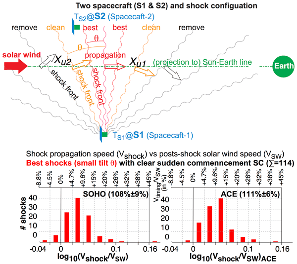
Figure 2(a) Definition of the η–ζ coordinate based on the alignment of two spacecraft looking from the Sun toward the Earth (looking from +XGSE). It is rotated by an angle ϕ of the alignment direction from the YGSE direction. (b) The spacecraft alignment direction at ζ=D plane (solid blue line) and its projection along the shock surface (tilted by angle θζ) to the ζ=0 plane (dashed blue line) are shown in the η–ζ coordinate. The shock surface in the ζ=0 plane is shown by the black wavy lines (which is tilted by angle θη). The signs of these angles are defined as the surface normal direction deflected from −XGSE direction toward positive η or positive ζ. (c) General configuration of the IP shocks (wavy lines), propagating (empty arrows) through two spacecraft (S1 and S2) that represent SOHO and ACE. Different colors represent different datasets (best, clean, and consistent) in terms of shock angle (θη) that is defined in Fig. 3b.
In Fig. 2b configuration, the propagation speed of the IP shock (Vshock) from the upstream point (, or ) to the Earth becomes the same between using the projected SOHO location (and shifted by distance with angle θζ in Fig. 2a) and using the projected ACE location to the upstream point (and shifted by distance D with angle θζ):
where the signs of θη and θζ are defined positive if the shock surface tilts from XGSE=constant plane toward positive η or positive ζ directions (see Fig. 2 caption), or
For the ζ direction, we have to rely on the other method, such as using a 1D shock model (θζ1D: Appendix A1), which has a large error range due to (a) inhomogeneity of the shock front that makes the local propagation speed quite different from the large-scale propagation speed, and (b) limited angular resolution of the ion instruments as described in the next subsection (Sect. 2.2). Therefore, in the statistical study, we select examples in which θζ is small compared to the measurement uncertainty that is described in Sect. 2.2. Fortunately, the second term in Eq. (2) (D⋅tan θζ term) is less than 0.3 for 99 % of 375 shocks (less than 0.1 for 93 %). In such cases, angle θζ disappears from Eqs. (1) and (2) as:
Using Eqs. (3) and (4), we can obtain Vtriangle and θη only from the timings and locations of the IP shock passage at two spacecraft. In the statistical analyses in this paper, we use these simplified formulae for Vtriangle and θη such that errors in the measured values (see below in Sect. 2.2) do not affect the result.
2.2 Accuracy of measurements
As is always the case with ion instruments, limited dynamic range of the sensor (for SOHO and ACE, it is microchannelplate (MCP)) causes saturation of the signal near and beyond the upper detection limit of the flux (ions entering the instrument too often beyond the sensor's capacity). In very high flux conditions such as during the passage of CME-driven IP shocks, saturation of the sensor causes underestimation of the flux and a shift of the central position in both energy and inflow angle. Among those, the energy (i.e., speed) is relatively well controlled (although the widening of the detecting energy causes some error in the energy) even during high-flux condition. Therefore, an underestimation of flux due to the saturation causes underestimation of the density (which is defined as the flux divided by speed). As shown in Appendix A2 (Fig. A1e), such underestimation causes a significant error in the theoretical propagation velocity when the change in the density is small. Therefore, we do not use density data in this study.

Figure 3(a) Scatter plot comparing the change in the solar wind deflection angle across the shock in the η direction and the shock angle in the in the η by the triangle method (θη, based on Eq. 2). (b) The same as (a) but for the deflection angle in the ζ direction, while the horizontal axis is the same (θη) except using Eq. (3). (c) Scatter plot comparing the shock angles in the η direction θη1D and θη (based on Eq. 2). (d) Scatter plot comparing the estimated errors in the shock angle in the η direction. Here we used Eq. (3) to derive the error in θη. The deflection angle is the angle that the solar wind is coming into the instrument measuring from the Sun direction. All three velocity components of the solar wind are calculated using the solar wind speed (eventually the energy) and these angles in the XGSE–YGSE and XGSE–ZGSE directions. The hatched area in (a) and (d) shows the “consistent” range between the triangle method (Sect. 2.1) and the 1D-model method (Appendix A1) after considering a 4° degree uncertainty in the deflection angle of the solar wind measurement (and 17° uncertainty in θη1D). The hatched areas (larger and smaller areas) in (b) shows selection criterions for “clean” and “best” shocks as summarized in Table 1, respectively, in selecting shocks propagating nearly along the −XGSE direction, i.e., small shock angle θ in both η and ζ directions.
Deflection angle (angle that the solar wind is coming into the instrument, measuring from the Sun direction) is another problem: the three-axis stabilized SOHO can measure the deflection of the solar wind only in the ZGSE direction but not in the YGSE direction at all (Ipavich et al., 1998). The solar wind instrument on board the spinning ACE spacecraft (spin period 12 s) has several entrance directions to cover the third direction (mainly in the ZGSE direction), but this 3D design sacrificed the angular resolution to 2.5–5° in the sector direction (the best resolution requires longer integration time) and 3–4.5° in the spinning direction, both after 1 min integration during stable solar wind conditions (McComas et al., 1998). The resolution during IP shock passage must be worse than these values.
Since tan (2.5°)=4.4 % and tan (4°)=7.0 %, a solar wind velocity of only 450 km s−1 (low values for the IP shock conditions) already gives 20–30 km s−1 uncertainty in the deflection (Y–Z) direction. Although NASA/OMNI dataset provides the Y–Z components of the solar wind velocity to the last digit, the uncertainty lies already in the tens of km s−1, making the final estimate for the error in the 1D-model shock angle (θη1D, see Appendix A) quite large. In contrast, the triangle method uses only the timing and location, with the time resolution (1 min) being the controlling factor determining the uncertainty in the estimate of θη.
Figure 3 shows scatter plots that compare the triangle method (horizontal axis) and the 1D-model method (vertical axis). Figure 3a compares the estimated shock angle in the η direction by the triangle method (θη) and the observed change in the solar wind deflection angle across the shock. If we include the instrumental uncertainty in the deflection angle of about 4° (hatched area), a majority of the observations is consistent to each other. Therefore, the value of 4° is a good estimate of the actual uncertainty in the deflection angle of the solar wind measurement in the η direction. Figure 3a also indicates that there are many shocks in which uncertainty in the deflection angle may be larger (wider area than the hatched area), as mentioned above.
After converting the change of the deflection angle across the shock to the shock angle by the 1D-model method, both estimates of the shock angle in the η direction (1D-model method θη1D and triangle method θη) are compared in Fig. 3c. We also estimated the error in these θη and θη1D by assuming 1-min error in Eq. (2) and 2.5° error (minimum possible error from the instrument design) of deflection angle in Eq. (A2). Figure 3d shows the result. The estimated uncertainty in the η direction is about five times larger for the 1D-model method than for the triangle method (medium values are 17° for the 1D-model method and 3.4° for the triangle method), contrary to the claim by Toth et al. (2026) who overlooked the large uncertainty in the velocity measurement. This endorses the error estimate of θη1D in Fig. 3c (hatched area, about ±20° error in θη1D). Since the uncertainty in the deflection angle comes from the instrumental design, we expect about the same uncertainty even in the ζ deflection angle (±4°), and hence in θζ1D (±20°).
If we have a third spacecraft, we can estimate the shock angle in both directions by the triangle method, but with two spacecraft, we have to relay on the 1D-model method in the ζ direction, which has such a large uncertainty. Fortunately, our purpose is just the large-scale propagation speed of the IP shocks and its uncertainty. Then, it is wise to use the angle information only to extract the “best” examples for which we can assume anti-sunward propagation nearly along the −XGSE direction. Note that the discrepancy between these two methods may also come from the difference between the large-scale shock angle and the small-scale shock angle, e.g., by curvature of the shock surface in both large scale (round) and small scale (wavy).
The hatched area in Fig. 3b shows this criterion for the clean dataset (261 shocks) and the best dataset (141 shocks), which are summarized in Table 1. A list of timings of the IP shock detection and geomagnetic SC for 438 IP shocks, including the classification of the difference sub-datasets, is listed in Appendix C (Tables C1–C4). The criterion in the ζ direction is slightly less restrictive than in the η direction because of large error range in the 1D-shock model, because a deflection angle of 4° is about 20° error in the shock angle according to Fig. 3a and c.


Figure 4Solar wind data observed by (a) SOHO and (b) ACE for the IP shock event on 1 January 2006. The proton speed, proton density, and the IMF intensity are plotted by thick black lines, thin blue lines, and a thin red line, respectively. As a reference, speed of the alpha particle is also plotted by a green line in the top panel. The IP shock is identified as sudden simultaneous intensification of the density and velocity for both SOHO (13:35 UT) and ACE (13:30 UT). The IMF total field measured by ACE also shows sudden intensification at the same timing (13:30 UT). (c) Geomagnetic indices SYM-H (thick black lines), ASY-H (thin red line), AU and AL (both thin blue lines) for the same IP shock. Sudden increase of SYM-H (and ASY-H and AU) is observed at 14:05 UT.
2.3 Example
Figure 4 shows an example of clean but not the best IP shock. Figure 4a and b show that a sudden sharp increase in the proton speed (thick black line) and density (thin blue line) occurred simultaneously for both SOHO at 13:35 UT (Fig. 4a) and ACE at 13:30 UT (Fig. 4b) on 1 January 2006. Also, the total IMF strength (dashed red line) observed by ACE suddenly increased simultaneously at 13:30 UT. Since the IP shock timing was identified as a sudden increase in dynamic pressure, the above timing corresponds to the IP shock timing passing through SOHO and ACE, respectively. Figure 4c shows that SYM-H suddenly increased at 14:05 UT as an isolated geomagnetic SC during a quiet period without any contamination from any magnetospheric activities (as seen from AU and AL indices). From the above timings, travel time of the IP shock is estimated as min for SOHO-Earth propagation and min for ACE-Earth propagation.
Let us estimate the propagation speed of the IP shock in the −XGSE direction. According to the simplified formulae Eqs. (3) and (4) and the location of the spacecraft given in Fig. 4, we have an estimate of ° and km s−1. This value is even consistent with the propagation speed using only one spacecraft assuming an ideal 1D shock propagating in −XGSE direction. The propagation time of 30±1 min over km means about km s−1, and 35±1 min over km means about km s−1). Also, the shock angle estimated by the 1D model (°) is consistent with the θη value by the triangle method above.
On the other hand, the tilt angle in the ζ direction (only 1D-model method can estimate) gives a large value of ° (the ζ deflection angle of the solar wind is 5.8±4°). While the corrected ° according to Eq. (2) is unchanged from the above simplified estimate, corrected Vtriangle according to Eq. (1) significantly decreased to ∼630 km s−1 with a large error range of ±50 km s−1 (the error range is ±30 km s−1 even if the uncertainty of the deflection angle is 2.5°). Thus, it is wise not to use the derived tilt angle to estimate Vtriangle but to select the best IP shocks (only small tilt angles), as summarized in Fig. 3b and Table 1.
In this example, the estimated km s−1 is much higher than the maximum solar wind speed of 520 km s−1 (the same value for both SOHO and ACE) observed within 15 min after the IP shock passage. For reference, we compare with the theoretical propagation speed in a simple 1D shock model (cf. Appendix A), although such an estimate requires density values (can be quite erroneous as discussed in Sect. 2.2). In fact, the density jumps across the shock in Fig. 4 are quite different between SOHO and ACE (nearly 4 times for SOHO and only double for ACE). The speed change is also different (from 470 to 520 km s−1 for SOHO and 440 to 520 km s−1 for ACE). Such a difference even suggests that the shock might be inhomogeneous in the η direction, as mentioned in Sect. 2.2.
With these limitations in mind, the estimated phase velocity of the shock in the −XGSE direction according to Eq. (A1) in Appendix A (540 km s−1 for SOHO and 600 km s−1 for ACE) is not very reliable. While estimation by the ACE data is within the uncertainty range of Vtriangle by the triangle method (required tile angle is >70°), estimation by the SOHO data is generally more reliable than the ACE estimate as discussed in Sect. 2.2 and Appendix A2.
In summary, the anti-sunward phase speed of the IP shock propagation on the 1 January 2006 event (estimated as ∼630 km s−1) is much faster than the solar wind (∼520 km s−1) as expected from the shock theory. However, we cannot use this example to “test” the theoretical model to derive the propagation speed (of ∼540 km s−1 based on SOHO density and velocity observations). The measurement uncertainties in the deflection angle and density are too high to judge if the discrepancy between these estimates comes from inhomogeneity, instrumental limitations, or other unknown reasons. This example encourages statistical examination of the shock propagation speed using the most reliable measurements (timing, distance, and solar wind energy or speed) rather than theoretical estimates using less reliable measurements and extra assumptions.
2.4 Statistical method
The purpose of the paper is to obtain the statistical difference between the shock propagation speed and the solar wind speed. To minimize the uncertainty introduced by the instrumental limitation, we use only the timing of the shock passage and the spacecraft location (XGSE, YGSE, ZGSE) in calculating the speed. For the same reason, we select ideal IP shocks from the 375 “consistent” examples according to Table 1 and Fig. 3b: those with the shock normal most likely pointing more or less in the −XGSE direction, as illustrated with red and orange empty arrows in Fig. 2c.
We first show the results when the finite YGSE and ZGSE is ignored (Figs. 5 and 6) because this is what is used for the real-time prediction of the arrival time in the space weather operation. Even with such assumption, we expect that the error introduced by this assumption is expected to be equally distributed to plus side and minus side, and may give some idea how fast the shock propagates compared to the solar wind.

Figure 5Histogram of the time difference Δt between the arrival times of the IP shock at the Earth using the geomagnetic SC signature in SYM-H (TSC), and the expected travel time of the solar wind using the fastest solar wind speed within 15 min from an IP shock for (a–c) SOHO and (d–f) ACE. Top panels (a) and (c) show the distributions of 375 “consistent” IP shocks, middle panels (b) and (e) show the distributions of 261 “clean” IP shocks, and bottom panels (c) and (f) show the distributions of 141 “best” IP shocks, as defined in Fig. 2 and Table 1. (g) The same histogram for removed samples from (a) to (b) for SOHO, i.e., difference between (a) and (b). In each panel, values at the upper right part show the 80 % range of the distribution, followed by the average value and the standard deviation. The values inside the parenthesis represent only those with the geomagnetic SC signature detected by two methods. The values at lower left and right edges show the summation of extreme values for both negative ( min) and positive ( min) sides, respectively. Positive Δt means that the actual arrival of the IP shock to the Earth is earlier than the predicted arrival time using the solar wind speed measured by SOHO or ACE. The data are classified into three types in terms of clearness of the SC signature in the same manner as Fig. 1a.
Figure 5 shows the statistics of the time difference Δt for SOHO (left panels) and ACE (middle panels). The format of each panel is the same as Fig. 1b. Figure 5a and d show the distributions of all 375 consistent IP shocks, Fig. 5b and e show the distributions of clean subset (261 samples), and Fig. 5c and f show the distribution of the best subset (141 samples), as is described in the previous section.
For both SOHO and ACE, Δt values of 375 consistent IP shocks (Fig. 5a and d) are distributed wide spread (central 80 % range and standard deviations (SD) are −2 to +15 min (SD = 7.2 min) for SOHO, and +2 to +13 min (SD = 5.6 min) for ACE). The distribution is more compact in the best dataset (Fig. 5c and f) with central 80 % range −1 min to +8 min with SD = 4.9 min for SOHO, and +1 to +9 min with SD = 3.4 min for ACE. The numbers of extreme Δt examples ( or >20 min) also decreases from 26 to 3 for SOHO and 11 to 1 for ACE for the best 141 examples compared to the consistent 375 examples. In fact, the removed examples (Fig. 5g) show much flatter distribution than clean and best example, consistent with wide error for oblique shocks as explained in the introduction.
In all panels, the center of Δt is shifted toward the positive side; i.e., the IP shock generally arrives earlier than the predicted arrival time calculated from the measured solar wind speed at L1, as is expected from the shock theory. The earlier arrival of the IP shock to the Earth than the solar wind itself is valid in almost all cases, and negative Δt is most likely a part of spread of the distribution, which is expected as the statistical property of the oblique shock plane, as explained in the introduction.

Figure 6The same as Fig. 5, but for the velocity ratio between the solar wind proton velocity (VSW) and the IP shock's propagation velocity (Vtiming). The latter is calculated using the time difference and XGSE distance between the IP shock passage at (a–c) SOHO or at (d–f) ACE, and the Earth (the geomagnetic SC signature is used for timing at the Earth). To linearize the binning of velocity ratio, we plotted in logarithmic scale. For example, −0.06 and 0.06 correspond to 87 % (i.e., 13 % slower propagation speed than the solar wind speed) and 115 % (i.e., 15 % faster), respectively. These differences are written at the top of each panel.
Figure 6 shows the velocity ratio for SOHO (left panels) and ACE (right panels) in the same format as Fig. 5, where VSW is the solar wind proton velocity and Vtiming is the IP shock's propagation velocity using only one spacecraft (the same assumption as Fig. 5). Since we consider the ratio, we linearized the binning by taking logarithmic scale; i.e., we plotted the distribution against log10(). The resultant distributions are similar to those of Δt in Fig. 5.
For the 141 best examples, Vtiming is −2 % to +18 % (central 80 %) faster (negative sign means slower) than the solar wind speed for SOHO (+3 % to +19 % for ACE), with the simple average and standard deviation of as 0.029 and 0.044 ( % difference) for SOHO as shown in Fig. 6c ( % difference for ACE, as shown in Fig. 6f).

Figure 7The same as Fig. 6, but instead Vtiming, using Vtriangle that is estimated according to Eqs. (3) and (4).
These averages are unchanged if we use Vtriangle (which is common for SOHO and ACE) instead of Vtiming for both SOHO and ACE, as shown in Fig. 7, where the results for Vtriangle (triangle method using two spacecraft) are shown instead of Vtiming. Even the standard deviation is nearly unchanged by using Vtriangle (reduced only by 2 % for SOHO and unchanged for ACE). However, the distribution with respect to the average value for SOHO case becomes more symmetric (Gaussian-like) by using Vtriangle than using Vtiming, with a reduced 80 % range. Contrary to the SOHO cases (Fig. 7a–c), ACE data show some asymmetry with respect to its peak, indicating less reliable velocity measurements than SOHO, as discussed in Sect. 2.2.
In all estimates using timings at L1 and the Earth to derive the propagation speed (Figs. 6 and 7), the shock propagation is faster than the solar wind flow, as is predicted from the shock theory for the forward shock (cf. Appendix A). The differences in the speed are about 7 % (0 % to +14 % for central 80 %) for SOHO and about 10 % (+3 % to +17 %) for ACE. For such small differences, we must consider possible sources of the uncertainty in the measurements (solar wind speed and timings) before using this value (about 7 % difference compared to the fastest solar wind speed within 15 min after the shock) as the value how fast the shock propagates.
4.1 Velocity value
One question is the accuracy of the velocity values. Although the SOHO proton monitor velocity is well calibrated against those measured by other SOHO instruments and other monitoring spacecraft such as Wind with a difference less than 1 % and a spread less than 3 % (e.g., Ipavich et al., 1998), the calibration is not made during the IP shock passage when the shock speed suddenly increases. In such conditions, a saturation effect is expected as mentioned in Sect. 2.2. Actually, the SOHO–ACE difference in Fig. 7 indicates that the measured speed behind the shock is smaller (difference is larger) by the ACE observation than by the SOHO observation. In other words, the saturation effect might underestimate the velocity change. However, Fig. 8 shows that the spread in does not depend very much on the solar wind speed, indicating that higher speed (higher risk of saturation) does not affect the VSW measurement.
Also, the small change in the shape of the distribution between Fig. 7b and c, both Gaussian-like, indicates that saturated cases are already removed in Fig. 7c, because the saturation effect may also deform the distribution asymmetric from the Gaussian-like distribution, as in the ACE case in Fig. 7f. In this respect, the solar wind speed (actually energy) of the SOHO measurement after the shock is reliable if we take the largest value within 15 min.
4.2 Change of speeds from L1 to the Earth
It is possible that an IP shock propagation is decelerated while the solar wind is accelerated, like the high-speed CME near the Sun (Yashiro et al., 2004). If the speed changes, we have to correct the solar wind speed to the average speed between L1 and the Earth, because the shock propagation speed is derived as an average value from start-end timings in this paper. Although the velocity measurements are statistically consistent between the L1 monitoring spacecraft and the Earth orbiting spacecraft (e.g., Ipavich et al., 1998), the same argument as above applies here (i.e., measurements near the IP shocks can be different from relatively constant solar wind). If such acceleration is substantial, the real offset in (and Δt) would be smaller than the present result. However, the distance from L1 to the Earth is only 1 % of the distance from the Sun to the Earth. We are not aware of any quantitative model that predicts substantial acceleration of the solar wind (or substantial deceleration of the IP shock) within such a short distance. Therefore, this is again less likely cause error in our results of 7 % difference between Vtriangle and VSW.
4.3 Transit time from the magnetopause to the Earth
The onset timing of the geomagnetic SC was used as the proxy of the timing when the IP shock passing the Earth's terminator. Considering about 105 km distance from the magnetopause to the Earth, the travelling time of the IP shock (speed of about 400–900 km s−1 as shown in Fig. 8) to the terminator is estimated about 1–3 min. On the other hand, the effect of the enhanced magnetopause current propagates to the Earth (to cause the geomagnetic SC) with about magnetosonic speed (not the speed of light), resulting in the similar travel time of 1–3 min. Therefore, the resultant uncertainty in Δt should be, if any, only 1–2 min.
If we are to improve the accuracy of Δt, we need to monitor the shock arrival at the magnetopause. The Smile satellite (Wang et al., 2025), recently launched in May 2026, monitors the magnetosheath solar wind with 0.5–2 s resolution, which is 20 times better than SOHO (Dai et al., 2025), at nearly the same location (apogee) for more than 40 h out of the nearly 2 d orbit. In addition, Smile can monitor the magnetopause compression using soft X-ray imaging (Sambay et al., 2025). Although the instrument design is 5 min resolution, this can go down to a few minutes for the arrival timing of the strong IP shocks. Then, we may still have a better accuracy of Δt if we have many IP shocks.

Figure 8(a) Scatter plot of the shock propagation speed Vtriangle against the post-shock solar wind speed observed by SOHO for the clean 261 IP shocks, where Vtriangle is estimated according to Eqs. (3) and (4). (b) The same as (a) but for the speed ratio (corresponding to Fig. 7b). Best 141 examples are marked by different symbols from the rest of clean examples.
4.4 Tilt of the shock front in the ζ direction
Using the triangle method (Eq. 3), we could estimate the tilt angle in the η direction (θη by the triangle method) with a small uncertainty, as shown in Fig. 3d. However, the estimated tilt angle in the ζ direction (we have only θζ1D by the 1D-model method) has a large error range because of a finite uncertainty in the solar wind defection angle (resultant uncertainty in the η–ζ components of the solar wind is not less than 20 km s−1). Although the resultant estimation error in the value should be equally distributed on both positive and negative sides, shape of the distribution is affected (longer tail toward higher values) as discussed in Sect. 4.1, causing a small effect even in the average value, as is seen from the decreasing average values with more filtering in Figs. 5, 6, and 7.
To minimize the influence by the large uncertainty in θζ1D, we used the estimated angles θη and θζ1D just for selecting the IP shocks of which the shock normal points nearly toward the −XGSE direction, such that the error caused by finite θ becomes relatively small. We defined the present criterion (Fig. 3b and Table 1) to keep total numbers of samples statistical liable. The success of the filtering is seen in Fig. 7a–c, where the distribution became more compact and symmetric after more selection. The difference in the scatter plot between the best cases and the rest of the clean cases in Fig. 8 is already small compared to the spread. Therefore, the average difference in the speed (7 %) would not decrease more than 1 % if a larger dataset allows us to tighten the criterion.
We examined IP shocks that have consistent velocity profiles between SOHO and ACE data during 1998–2022. To remove IP shocks with shock surface largely tilted from the YGSE–ZGSE direction, we estimated the tilt angle in the XGSE–η–ζ coordinate in Fig. 2, where the η is parallel to the projected two-spacecraft alignment direction on the YGSE–ZGSE plane. In this coordinate, the tilt angle in the η direction (θη) is estimated by the triangle method (Eq. 3). For the ζ direction, we used the change in the deflection angle in the ζ direction across the shock, which is more close to the raw data than the estimate θζ1D by the simple 1D shock model (Eq. A2). The criterions of selecting IP shocks propagating nearly along the −XGSE directions (the clean shocks and the best shocks) are given in Fig. 3b and Table 1.
Statistics of the IP shock during 1998–2022 shows that the geomagnetic SC takes place generally earlier than the predicted solar wind arrival time using the measured solar wind speed at L1 (even using the highest proton speed within 15 min after the IP shock passage). Thus, as is expected from the shock theory, the IP shocks observed by SOHO and ACE propagate to the Earth faster than the solar wind.
For the 141 “best” IP shocks propagating nearly along the −XGSE direction, the time difference Δt (positive value for earlier geomagnetic SC) spreads over −1 to +10 min (central 80 % range) for SOHO and +2 to +8 min for SOHO, with a finite number of IP shocks (8 shocks for SOHO and 5 shocks for ACE out of 141 samples) arrived more than 10 min earlier than the predicted solar wind arrival time as shown in Fig. 5c and f. The corresponding propagation speed of the IP shock derived by the triangle method (Eq. 4) for the best 141 shocks is 7 % faster than the solar wind speed for SOHO (10 % for ACE), with individual values ranging from 0 % to +14 % (+3 % to +17 % for ACE), as shown in Fig. 7c and f. If the propagation speed (Vtiming) is estimated from the timing and XSGE distance of the spacecraft, the distribution is more widespread and more asymmetric from the Gaussian-like distribution for SOHO, as shown in Fig. 6c.
Let us compare the average differences between the IP propagation speed and the solar wind speed (about 7 %) with the simple 1D shock model (Eq. A1 in Appendix A). Here one must note that the model requires density and normal velocity to the shock of both before and after the shock passage (four measured values) instead of only post-shock speed (one measured value) for Vtriangle, and that the resultant shock propagation speed V1D is very sensitive to the density ratio between before and after the shock, particularly when the ratio is near unity, as shown in Fig. A1e in Appendix A2. Considering that the post-shock density values can be underestimated due to possible saturation of the instrument (cf. Sect. 2.2), the calculated V1D can be significantly overestimated when the density ratio is close to unity. This effect is seen in the sparse spread of values in Fig. A2 in Appendix A (this is why we show this figure in Appendix rather than in the main text).
Removing these overestimated cases, Fig. A2 indicates that a simple 1D model has the dense cluster of around +10 %, which is consistent with the observed speed (), although individual cases are not well correlated. This indicates that the simple 1D model is a good guide in estimating the shock propagation speed near the Earth, encouraging development of the solar wind measurement method (both density and deflection angle), particularly right after the shock, as well as placing three or more spacecraft near the L1 region.
If only one spacecraft is used, the spread of Δt is as wide as Fig. 1 (and Fig. 5a) due to the oblique shock front (cf. Figs. 2c and 5g), with a substantial fraction arriving >10 min earlier than the predicted time. This means that one must be ready for possible space weather hazard starting earlier than the predicted arrival time based on the real-time L1 monitor, although one can expect, in average, the shock propagation about 1.1 times faster than the observed solar wind speed. This fact also warns the usage of 1 min resolution solar wind OMNI data at the magnetopause (https://omniweb.gsfc.nasa.gov/, last access: 16 June 2026), in which the same propagation speed as the measured solar wind speed is used when projecting the L1 observation to the magnetopause nose (Omniweb, 2026).
As is expected from the shock theory, the IP shocks observed by SOHO and ACE propagate to the Earth faster than the solar wind. We used two spacecraft instead of one to select nearly radially propagating IP shocks (shock normal is not tilted very much from the −XGSE direction) through two selecting parameters (equivalent to the shock angle in two directions) shown in Figs. 2c and 3b. For the best 141 shock that are selected in this manner, the shock propagate faster than solar wind speed measure by SOHO (maximum value within 15 min after the shock) by about 7 % in average with standard deviation of 9 % (average 10 % with standard deviation of 7 % for ACE).
The shock tilt angle that is estimated by simple 1D shock model using velocity change across the shock of ACE gives, although this method has large instrumental uncertainty, generally consistent value with what is estimated by the triangle method in the spacecraft alignment direction within that large uncertainty. The same applies even for the propagation speed, although the 1D-model method has even larger instrumental uncertainty.
Figure A1 illustrates the mass flux conservation relation for a textbook-type 1D shock. Through conservation relation in the shock frame, the density n and velocity normal to the shock v in the spacecraft frame has a relation of
or
where is inverse of the shock compression ratio, and suffix “a”, “b”, and “1D” denote after the shock passage, before after the shock passage, and shock front, respectively.

Figure A1(a, b) Illustration of mass flux (n⋅v, where n is density and v is 1D speed) conservation across the simplest 1D shock in (a) spacecraft rest frame and (b) shock rest frame. (c, d) A more general 1D shock case with finite flow velocity along the shock surface. To distinguish this direction from GSE (YGSE) or spacecraft alignment coordinate (η) in Fig. 2, we use small y to denote this direction. (e) Theoretical values (ratio between the shock propagation speed V1D and the flow speed after the shock va) is plotted against (inverse of the shock compression ratio) for different velocity changes. Suffix “a”, “b”, and “1D” in the upper panel denote after the shock passage, before the shock passage, and shock front, respectively. Suffix “in” and “out” in the lower panel denote the inflow to the shock and outflow from the shock, respectively.
A1 1D-model shock angle θη1D and θζ1D
This relation is unchanged when the flow component along the shock front (vy) is added (cf. Fig. A1c and d), as long as vy is the same between the upstream and downstream (i.e., no vorticity is carried by the shock, which is normally the case for high Alfvén Mach number shocks). In this case, the shock normal direction n is approximately
where is the change in the solar wind velocity across the shock in the spacecraft frame, and θ is the shock angle (e.g., Paschmann and Daly, 1999 Eq. 10.18). In the present paper, we use and in Eq. (A2) (propagation direction toward −XGSE determines the sign in the present definition of θη and θζ1D) when comparing with the triangle method in Sect. 2.2.
The propagation speed in the shock normal direction V1D is approximately
where θ is the shock angle (e.g., Paschmann and Daly, 1999, Eq. 10.29), while the earthward phase velocity becomes the same as Eq. (A1).
A2 Density underestimation effect in deriving the propagation speed
Although Eq. (A1) provides , one cannot simply trust the derived values in the actual shock observations because of the high uncertainty in the solar wind measurement (particularly density) right after the shock: na (and possibly va) can be significantly underestimated due to saturation of the ion instrument, as explained in Sect. 2.2. This makes overestimation of the values for some shocks, making them much closer values to unity than it actually is. As shown in Fig. A1e, the value is very sensitive to value near , making small underestimation of na resulting in large overestimation of V1D (and ). This is why we did not show the distribution plots of .
Figure A2 shows scatter plots comparing theoretical 1D shock speed V1D using density and velocity values of SOHO both before and after the shock (according to Eq. A1) and measured Vtriangle between L1 and Earth based on Eq. (4). Since the density is more variable than the velocity, we took average values over 10 min periods for the solar wind values in Fig. A2: 3–13 min before the shock and 3–13 min after the shock. Nevertheless, there are several cases when the density values superficially decreased after the shock even it is forward shock according to the ACE data. We removed such obvious cases of unreliable density data as well as the reverse shocks in Fig. A2. After normalized by VSW (Fig. A2b), values of and fall into the same range (majority around +10 %) although individual cases are not well correlated to each other.
We also examined the effect of tilt angle (η and particularly ζ) by subdividing the dataset into the best examples and rest of the clean examples (i.e., larger angle than the best examples). After removing obviously overestimated cases, no outstanding difference is seen between them. As is already seen in Fig. 7, selecting the best cases makes the distribution in the horizontal direction more compact than all clean cases, but not in the vertical axis ().

Figure A2Scatter plot of 228 clean examples of forward shocks (selected from the 261 clean shocks) between V1D according to Eq. (A1) and velocity values of SOHO both before and after the shock and the measured Vtriangle according to Eq. (4): (a) V1D against VSW; (b) against (comparing the normalized speed). The solar wind values used in these specific plots are 10 min average values over 3–13 min before the shock and 3-13 min after the shock. Different symbols mean the different dataset defined by Table 1. We further limited the dataset to those with clear forward shock and with clear geomagnetic SC signature (seen two different methods).
Figure 2a shows the η–ζ coordinate system that is tilted by angle ϕ from the YGSE–ZGSE coordinate system, where ϕ is the SOHO-ACE alignment direction in the YGSE–ZGSE plane. After a rotation by ϕ, a coordinate (YGSE, ZGSE) and a vector (vY, vZ) are expressed in the η–ζ coordinate as
In the configuration of Fig. 2a, the η axis is parallel to the alignment between (Y1, Z1) and (Y2, Z2) in the YGSE–ZGSE plane with distance . Therefore, we have a relation
and final conversion formulae
Table C1 lists the timings of the best 141 IP shocks (see Table 1) that are used in the statistical study. The second and third columns show the UT of IP shock detection by SOHO and by ACE, respectively. The fourth column shows the onset UT of sudden increase of SYM-H. The last column indicates the clearness of the SC (see caption of Fig. 1).
In the same format, Table C2 lists the timings of the remaining 120 IP shocks other than the best 141 shocks (after removing the samples listed in Table C1) out of 261 “clean” IP shock in Table 1.
Similarly, Table C3 lists the timings of the remaining 114 IP shocks (after removing the samples listed in Tables C1 and C2) out of 375 “consistent” IP shock on Table 1.
Finally, Table C4 lists the timings of the 63 IP shocks with only SOHO data (after removing the samples listed in Tables C1–C3) out of 438 “basic samples” IP shock in Table 1.
Table C1Timing of IP detection and geomagnetic SC for “best” 141 samples.

a Identification of geomagnetic SC by both methods (=2), by only SYM-H (=1), and weak/unclear SC (=?). b Reverse shock. c Density measurement is skeptical.
Table C2Timing of IP detection and geomagnetic SC for “clean” 120 samples.

a Identification of geomagnetic SC by both methods (=2), by only SYM-H (=1), and weak/unclear SC (=?). b Reverse shock. c Density measurement is skeptical.
Table C3Timing of IP detection and geomagnetic SC for very oblique 114 samples.

a Identification of geomagnetic SC by both methods (=2), by only SYM-H (=1), and weak/unclear SC (=?). b Reverse shock. c Density measurement is skeptical.
Table C4Timing of IP detection and geomagnetic SC for SOHO-only 63 samples.

a Identification of geomagnetic SC by both methods (=2), by only SYM-H (=1), and weak/unclear SC (=?). b Reverse shock. c Density measurement is skeptical.
SOHO data is taken from SOHO site (https://l1.umd.edu/, last access: 16 June 2026) and NASA NASADCC site (https://cdaweb.gsfc.nasa.gov/, last access: 16 June 2026). ACE data is taken from both ACE site (https://izw1.caltech.edu/ACE/ASC/level2/index.html, last access: 16 June 2026) and NASA NASADCC site (https://cdaweb.gsfc.nasa.gov/, last access: 16 June 2026). Geomagnetic indices are taken WDC-C2 for geomagnetism, Kyoto University (https://wdc.kugi.kyoto-u.ac.jp/wdc/Sec3.html, last access: 16 November 2026). Another list of geomagnetic sudden commencement is found at Ebre Observatory data portal (https://www.obsebre.es/en/variations/rapid, last access: 16 November 2026).
MY and YY initiated the work. YY made overview plots related to SOHO and ACE in several format for all the events, and prepared tables that contain the velocity, timing, and the expected transit time. MY made the sub-dataset of the geomagnetic SYM-H indices (SYMASY) to identify the onset timing of geomagnetic SC timing, and examined all these plots to revise and complete the table made by YY. TK mainly contributed to SYM-H part, and JM made independent SC list from different dataset. MY made first draft of the text and figures, while all others contributed the text and discussion.
The contact author has declared that none of the authors has any competing interests.
Publisher's note: Copernicus Publications remains neutral with regard to jurisdictional claims made in the text, published maps, institutional affiliations, or any other geographical representation in this paper. The authors bear the ultimate responsibility for providing appropriate place names. Views expressed in the text are those of the authors and do not necessarily reflect the views of the publisher.
SOHO is a project of international cooperation between ESA and NASA. ACE is a NASA project that is aimed as the solar wind monitor during the International Solar Terrestrial Program. Data from both spacecraft are open access. The authors gratefully thank the instrument teams that maintained the quality of the solar wind data at L1 for nearly 30 years that are used in this study: SOHO PM team (PI: F. M. Ipavich), ACE SWEPAN team (PI: D.J McComas), and ACE MG team (PI: N. Ness). The NASA OMINI data at Omniweb site is maintained by Space Physics Data Facility, NASA Goddard Space Flight Center.
Geomagnetic indices SYMASY and AE are calculated by World Data Center (WDC) for Geomagnetism, Kyoto using geomagnetic field data at SYMASY stations (San Juan, Fredericksburg, Boulder, Tucson, Papeete, Honolulu, Memambetsu, Urumqi, Alma Ata, Alibag, Martin de Vivies, Hermanus, Chambon-la-Foret) and AE stations (Abisko, Amderma, Dixon Island, Cape Chelyuskin, Tixie Bay, Pebek, Cape Wellen, Barrow, College, Yellowknife, Fort Churchill, Sanikiluaq, Great Whale River, Poste-de-la-Baleine, Narsarsuaq, Leirvogur). The geomagnetic SC list at Ebre Observatory is derived from geomagnetic field data at many stations listed there. We thank all these contributing observatories.
Special thank goes to T. Araki (deceased August 2025) who initiate another work for which the produced plots lead this work. Without him, we never started this work. MY is partly supported by Swedish National Space Agency (dnr 2024-00124).
This research has been supported by the Swedish National Space Agency (grant no. 2024-00124).
The publication of this article was funded by the Swedish Research Council, Forte, Formas, and Vinnova.
This paper was edited by Dalia Buresova and reviewed by Gabor Toth and one anonymous referee.
Araki, T.: Global structure of geomagnetic sudden commencements, Planet. Space Sc., 25, 373–384, https://doi.org/10.1016/0032-0633(77)90053-8, 1977. a
Araki, T.: A Physical Model of the Geomagnetic Sudden Commencement, 183-200, American Geophysical Union (AGU), ISBN 9781118663943, https://doi.org/10.1029/GM081p0183, 1994. a
Collier, M. R., Slavin, J. A., Lepping, R. P., Szabo, A., and Ogilvie, K.: Timing accuracy for the simple planar propagation of magnetic field structures in the solar wind, Geophys. Res. Lett., 25, 2509–2512, https://doi.org/10.1029/98GL00735, 1998. a, b
Dai, L., Kong, L., Zhang, A., Kataria, D., Berthomier, M., Gao, J., Su, B., Escoubet, C. P., Wang, C., Li, L., Ren, Y., Wang, W., Lv, Y., Ding, J., Nicolaou, Ge., Wurz, P., Raab, W., Vey, S., and Echim, M.: The light ion analyzer (LIA) for the SMILE mission, Space Sci. Rev., 221, 109, https://doi.org/10.1007/s11214-025-01235-w, 2025. a
Gonzalez-Esparza, A. and Aguilar-Rodriguez, E.: Speed evolution of fast CME/shocks with SOHO/LASCO, WIND/WAVES, IPS and in-situ WIND data: analysis of kilometric type-II emissions, Ann. Geophys., 27, 3957–3966, https://doi.org/10.5194/angeo-27-3957-2009, 2009. a
Gopalswamy, N., Yashiro, S., Michalek, G., Stenborg, G., Vourlidas, A., Freeland, S., and Howard, R.: The SOHO/LASCO CME Catalog, Earth, Moon, Planet., 104, 295–313, https://doi.org/10.1007/s11038-008-9282-7, 2009. a
Ipavich, F. M., Galvin, A. B., Lasley, S. E., Paquette, J. A., Hefti, S., Reiche, K.-U., Coplan, M. A., Gloeckler, G., Bochsler, P., Hovestadt, D., Grünwaldt, H., Hilchenbach, M., Gliem, F., Axford, W. I., Balsiger, H., Bürgi, A., Geiss, J., Hsieh, K. C., Kallenbach, R., Klecker, B., Lee, M. A., Managadze, G. G., Marsch, E., Möbius, E., Neugebauer, M., Scholer, M., Verigin, M. I., Wilken, B., and Wurz, P.: Solar wind measurements with SOHO: The CELIAS/MTOF proton monitor J. Geophys. Res., 103, 17205–17213, https://doi.org/10.1029/97JA02770, 1998. a, b, c, d, e
King, J. and Papitashvili, N.: Explanation of one min and 5-min solar wind data sets at the Earth's bow shock nose of OMNIWeb, https://omniweb.gsfc.nasa.gov/html/omni_min_data.html#3 (last access: 12 February 2026), 2025. a
Manoharan, P. K., Tokumaru, M., Pick, M., Subramanian, P., Ipavich, F. M., Schenk, K., Kaiser, M. L., Lepping, R. P., and Vourlidas, A.: Coronal mass ejection of 2000 July 14 flare event: Imaging from near-Sun to Earth environment, Astrophys. J., 559, 1180–1189, https://doi.org/10.1086/322332, 2001. a
McComas, D. J., Bame, S. J., Barker, P., Feldman, W. C., Phillips, J. L., Riley, P., and Griffee J. W.: Solar Wind Electron Proton Alpha Monitor (SWEPAM) for the Advanced Composition Explorer, Space Sci. Rev., 86, 563–612, https://doi.org/10.1023/A:1005040232597, 1998. a, b, c
Milan, S. E., Carter, J. A., Bower, G. E., Fleetham, A. L., and Anderson, B. J.: Influence of off-Sun–Earth line distance on the accuracy of L1 solar wind monitoring, J. Geophys. Res., 127, e2021JA030212, https://doi.org/10.1029/2021JA030212, 2022. a
Nanjo, S., Yamauchi, M., Johnsen, M. G., Yokoyama, Y., Brändström, U., Ogawa, Y., Willer, A. N., and Hosokawa, K.: Leaping and vortex motion of the shock aurora toward the late evening sector observed on 26 February 2023, Ann. Geophys., 43, 303–317, https://doi.org/10.5194/angeo-43-303-2025, 2025. a
Ogilvie, K. W., Chornay, D. J., Fritzenreiter, R. J., Hunsaker, F., Keller, J., Lobell, J., Miller, G., Scudder, J. D., Sittler, E. C., Torbert, R. B., Bodet, D., Needell, G., Lazarus, A. J., Steinberg, J. T., Tappan, J. H., Mavretic, A., and Gergin, E.: SWE, a comprehensive plasma instru- ment for the WIND spacecraft, Space Sci. Rev., 71, 55–77, https://doi.org/10.1007/BF00751326, 1995. a
NASA Goddard Space Flight Center: Omniweb Plus, https://omniweb.gsfc.nasa.gov/ (last access: 16 June 2026), 2026. a
Paschmann, G. and Daly, P. W. (Eds.): Analysis Methods for Multi-Spacecraft Data, ISSI Scientific Reports, ESA Publ. Div., Noordwijk, the Netherlands, https://www.issibern.ch/PDF-Files/analysis_methods_1_1a.pdf (last access: 16 November 2026), 1999. a, b, c
Paularena, K. I., Zastenker, G. N., Lazarus, A. J., and Dalin, P. A.: Solar wind plasma correlations between IMP 8, INTERBALL-1 and WIND, J. Geophys. Res., 103, 14601–14617, https://doi.org/10.1029/98JA00660, 1998. a
Paularena, K. I., Richardson, J. D., Zastenker, G. N., and Dalin, P. A.: Solar wind correlations: Using a solar wind monitor successfully, in: Interball in the ISTP Program, edited by: Sibeck, D. G. and Kudela, K., NATO Science Series, vol 537. Springer, Dordrecht, https://doi.org/10.1007/978-94-011-4487-2_12, 1999. a
Richardson J. D. and Paularena, K. I.: The orientation of plasma structure in the solar wind, Geophys. Res. Lett., 25, 2097–2100, https://doi.org/10.1029/98GL01520, 1998. a
Sembay, S., Cheney, A., Hampson, R., Agnolon, D., Arnold, T., Beardmore, A., Balado, A., Bicknell, C., Bouldin, C., Branduardi-Raymont, G., Breuer, J. P., Buggey, T., Butcher, G., Canchal, R., Carter, J. A., Collada-Vega, Y., Connor, H., Crawford, T., Curry, P., Eaton, N., Feldman, C., Forsyth, C., Galgóczi, G., Garcia, J., Genov, G., Giono, G., Gordillo, C., Gröbelauer, H.-P., Guedel, M., Hailey, M., Halain, J.-P., Hall, D., Hansford, G., Hasiba, J., Hetherington, O., Hoffman, K., Holland, A., Hsieh, S.-Y., Hubbard, M. W. J., Jeszenszky, H., Jones, M., Kennedy, T., Koch-Mehrin, K., Koegl, S., Krucker, S., Kuntz, K., Kürbisch, C., Lakin, C., Laky, G., Leach, S., Leichtfried, M., Luntzer, A., Linder, D., Maddi, V., Martindale, A., Mas Hesse, J. M., Mecina, M., Nakamura, R., Neukirchner, S., Oksavik, K., Østgaard, N., Ottacher, H., Ottensamer, R., Pagani, C., Parsons, S., Patel, P., Pearson, J., Peikert, G., Porter, F. S., Qureshi, B. H., Raab, W., Read, A., Reading, I., Rostad, M. E., Runciman, C., Sachdev, S., Samara-Ratna, P., Samsonov, A., Sibeck, D., Søndergaard, J., Smit, S., Soman, M., Speight, R., Stavland, S., Steinberger, M., Steller, M., Sun, T., Sykes, J., Thomas, W., Thornhill, J., Tonfat Seclen, J., Tvaruzka, A., Ullaland, K., Wallner, R., Walsh, B., Walton, D., Wang, C., Willis, G., and Yang, S.: The soft X-ray imager (SXI) on the SMILE Mission, Space Sci. Rev., 221, 113, https://doi.org/10.1007/s11214-025-01241-y, 2025. a
Tokumaru, M., Kojima, M., Fujiki, K., and Yamashita, M.: Tracking heliospheric disturbances by interplanetary scintillation, Nonlin. Processes Geophys., 13, 329–338, https://doi.org/10.5194/npg-13-329-2006, 2006. a
Toth, G., Dredger, P., and Pulkkinen, T.: Michigan geospace model with ensemble forecasting and particle filtering: Modeling the May 2024 extreme storm, Space Weather, 24, e2026SW005083, https://doi.org/10.1029/2026SW005083, 2026. a
Wang, C., Branduardi-Raymont, G., Escoubet, C. P., and Forsyth, C.: Solar wind magnetosphere ionosphere link explorer (SMILE): Science and mission overview, Space Sci. Rev., 221, 9, https://doi.org/10.1007/s11214-024-01126-6, 2025. a
Yashiro, S., Gopalswamy, N., Michalek, G., St. Cyr, O. C., Plunkett, S. P., Rich, N. B., and Howard, R. A.: A catalog of white light coronal mass ejections observed by the SOHO spacecraft, J. Geophys. Res., 109, A07105, https://doi.org/10.1029/2003JA010282, 2004. a, b
- Abstract
- Introduction
- Data and Method
- Results
- Possible error sources
- Summary and Discussion
- Conclusions
- Appendix A: 1D-shock mass flux conservation relation
- Appendix B: Conversion from YGSE-ZGSE coordinate to η–ζ coordinate
- Appendix C: Timing list of IP shocks
- Data availability
- Author contributions
- Competing interests
- Disclaimer
- Acknowledgements
- Financial support
- Review statement
- References
- Abstract
- Introduction
- Data and Method
- Results
- Possible error sources
- Summary and Discussion
- Conclusions
- Appendix A: 1D-shock mass flux conservation relation
- Appendix B: Conversion from YGSE-ZGSE coordinate to η–ζ coordinate
- Appendix C: Timing list of IP shocks
- Data availability
- Author contributions
- Competing interests
- Disclaimer
- Acknowledgements
- Financial support
- Review statement
- References