Reevaluation of EISCAT plasma parameters during the May 2024 geomagnetic storm using O⁺ ratios from AMIE-driven SD-WACCM-X

We present a reevaluation of EISCAT plasma parameters during the May 2024 geomagnetic storm, applying the ion composition from an AMIE-driven SD-WACCM-X simulation instead of the standard IRI model. This resulted in significant deviations of F1 region electron densities (up to 15 %), electron temperature (40 %), and ion temperatures (30 %) from the original analysis. Parameter uncertainties are also shown to be affected by the reevaluation (5 %–10 %). The correlations of parameter uncertainty, ion composition differences, and absolute ion composition profiles are investigated. It is shown that in the F1 region, the plasma parameter deviations are notably larger than the uncertainty range. Incorrect assumptions about the ion composition can have a significant impact on the accuracy of ISR measurements, which has important consequences for the possible application of ISR data in data assimilation. Advantages and disadvantages compared to previously presented approaches regarding the ion composition issue are discussed. The presented method allows to de-bias storm-time ISR measurements with standard analysis software. Whether a generally applicable empirical model, which would allow for de-biasing without additional incoherent scatter analysis, can be derived with the presented method remains to be investigated in the future.

1 Introduction

Incoherent Scatter Radar (ISR) measurements are a crucial component of many space weather studies, as they provide multiple ionosphere parameters, including electron density, ion/electron temperature, and ion velocity. However, these parameters are inferred from the incoherent scatter spectrum, assuming certain a priori parameters, most notably the ratio of atomic oxygen ion (O⁺) density to the electron density, N_e. It has been shown in the past that the assumed ion composition has a considerable effect on the electron and ion temperature measurements (e.g. Blelly et al., 2010; Zettergren et al., 2011; Martínez-Ledesma and Díaz Quezada, 2019; Virtanen et al., 2021; Günzkofer et al., 2025b). Hence, the measurement reliability is strongly affected by the accuracy of the a priori modeled O⁺ ratio profile.

The most commonly applied empirical ionosphere model is the International Reference Ionosphere (IRI, Rawer et al., 1978). Bilitza et al. (2022) gives an overview of the different IRI versions and applied parameterizations. They note that the accuracy of empirical ion composition models is significantly limited by the scarcity of measurements, especially for statistically rare conditions, e.g. during geomagnetic storms. Physics-based thermosphere-ionosphere models obtain the ion composition by solving the continuity and momentum equations of the ionosphere (Sojka, 1989). However, though the ion chemistry in the F region is considerably simpler than in the D and E regions (Rishbeth and Garriott, 1969), plasma dynamics and thermosphere-ionosphere coupling affect the accuracy of the modeled ion composition (e.g. Zettergren et al., 2010; Huba et al., 2021; Lee et al., 2024). Nevertheless, physics-based ionosphere models are likely to cover the variability of the F region ion composition better than empirical models for geomagnetically active periods.

To assess the effects of empirical and physics-based model ion compositions, we reevaluate the ISR measurements with the EISCAT Svalbard Radar during the major geomagnetic storm in May 2024 (Themens et al., 2024; Cai et al., 2026). For this reevaluation, we replace the O⁺ ratios given by the default ionosphere a priori model (IRI2020) of the EISCAT analysis with the O⁺ ratios as given by the physics-based Whole Atmosphere Community Climate Model with thermosphere/ionosphere extension (WACCM-X). Different high-latitude drivers of the WACCM-X model are compared.

Section 2 gives an overview of the applied measurements and models. Section 3 shows the reevaluated plasma parameters and relates them to the model differences in O⁺ ratio. Section 4 discusses the obtained results, and the advantages and disadvantages of the technique applied in this paper compared to previous solutions of the ion composition issue. Section 5 summarizes the main conclusion and gives an outlook on future work.

2 Measurements and models

2.1 EISCAT Svalbard Radar

The EISCAT Svalbard Radar (ESR) is located at 78.2° N, 16.1° E, inside the polar cusp, and has been in operation for nearly 30 years (Wannberg et al., 1997; Baddeley et al., 2023). It operates at a radar frequency of 500 MHz and consists of two parabolic receive antennas: one fully steerable with a 32 m diameter and one fixed along the local geomagnetic field direction, with a 42 m diameter. During the major geomagnetic storm in May 2024, the ESR was continuously operated from 10 May 13:00 UTC to 14 May 12:00 UTC in the ipy_fixed42m mode. This means that only the 42 m antenna was utilized and, hence, all measurements are conducted at 81.6° elevation along the local magnetic field. More information about EISCAT instruments and operation modes can be found in Tjulin (2025).

To obtain plasma parameters, EISCAT measurements are analyzed with the Grand Unified Incoherent Scatter Design and Analysis Package GUISDAP (Lehtinen and Huuskonen, 1996). We leverage the GUISDAP version 9.2 (Häggström, 2021), which includes the IRI2020 (Rawer et al., 1978; Bilitza et al., 2022) and the NRLMSIS 2.1 (Emmert et al., 2022) to generate an a priori state of the atmosphere-ionosphere system. The GUSIDAP sub-function, which calls the ionosphere a priori model, was modified to acquire the O⁺ ratio from a previously prepared input file for reevaluation. The autocorrelation function of the radar signal was integrated over 300 s for each analysis step. This is considerably longer than the default 60 s integration period, but was chosen to match the output frequency of the whole-atmosphere model (see Sect. 2.2).

2.2 SD-WACCM-X

WACCM-X is a whole-atmosphere model developed and maintained by the National Center for Atmospheric Research (Liu et al., 2018). SD-WACCM-X is the specified dynamics model configuration, which means that lower atmosphere dynamics are nudged to the MERRA2 reanalysis (Rienecker et al., 2011). SD-WACCM-X has been validated and applied in multiple previous studies (e.g. Stober et al., 2021; Hindley et al., 2022; Günzkofer et al., 2022; Shi et al., 2025).

The model run applied for the present study was conducted at approximately 1.9°×2.5° latitude-longitude and 0.25 scale heights vertical resolution. Instantaneous outputs of the basic atmosphere-ionosphere parameters, including the ion composition, were written in 5 min intervals to obtain a maximum time resolution while keeping the computational cost and data amount reasonable.

Specifying the geomagnetic forcing of thermosphere-ionosphere models is an important issue, since it has been shown that different models for the high-latitude electrodynamics result in considerably different thermosphere-ionosphere conditions (Günzkofer et al., 2024, 2025a). The “default” choice is empirical models of the high-latitude convection pattern. However, data assimilative methods are generally considered to result in a more realistic geomagnetic forcing, but are also more difficult to obtain compared to standard empirical models. We will compare the O⁺ ratios from two WACCM-X runs, driven with the empirical Heelis convection model (Heelis et al., 1982) and the Assimilative Mapping of Ionospheric Electrodynamics (AMIE, Richmond and Kamide, 1988). The Heelis model applies the 3-hourly Kp index for parameterization. For the May 2024 superstorm, the AMIE assimilation includes measurements by the SuperDARN radar network, the SuperMAG magnetometer network, DMSP satellite measurements of ion drift, DMSP/SSUSI measurements of auroral precipitation, as well as AMPERE and Swarm (A and B) satellite magnetic field data.

3 Results

The major geomagnetic storm of May 2024 was the strongest space weather event in two decades and reached the maximum possible Kp=9 index (the Kp-similar Hp30 index, for which no upper limits apply, reached up to 11.33). A complete overview of the storm impact at high latitudes can be found in Themens et al. (2024). In addition, Cai et al. (2026) studied the polar ionosphere-thermosphere coupling using multiple observations. They showed that both T_i increases and neutral composition changes are important for F region recombination and hence result in electron density depletion and ion composition changes in the polar region. The geomagnetic storm started at about 17:00 UTC on 10 May and reached its maximum during the night from 10–11 May. On 11 and 12 May, Themens et al. (2024) and Cai et al. (2026) showed a strongly pronounced negative storm phase, indicating significant thermospheric upwelling and consequent disturbances of the chemical composition at the thermosphere/ionosphere. Figure 1 shows the EISCAT ESR measurements of electron density N_e, electron temperature T_e, and ion temperature T_i from 10–13 May 2024.

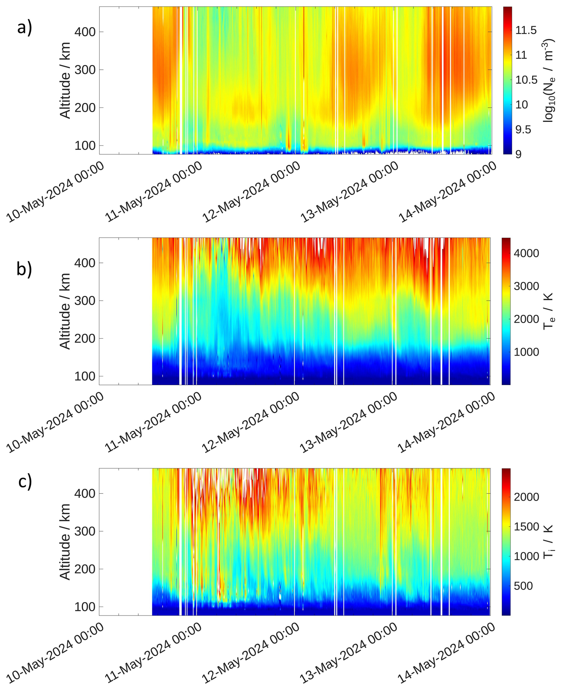
Figure 1 EISCAT ESR measurements of (a) electron density, (b) electron temperature, and (c) ion temperature from 10–13 May 2024.

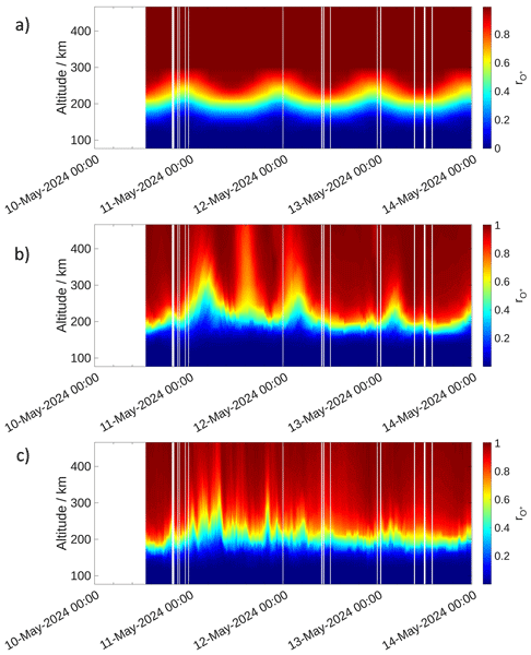
As described in Sect. 2.1 and Günzkofer et al. (2025b), the plasma parameters in Fig. 1 are inferred from the incoherent scatter spectrum assuming certain a priori parameters from the empirical IRI 2020 and NRLMSIS 2.1 models. Figure 2a shows the O⁺-to-N_e ratio $r_{{\mathrm{O}}^{+}}$ as given by the IRI model from 10–13 May 2024. It can be seen that IRI provides the diurnal variation of $r_{{\mathrm{O}}^{+}}$ but no variations as expected from the varying geomagnetic conditions during this period. The Heelis- and AMIE-driven WACCM-X O⁺ ratios in Fig. 2b and c show this variation of $r_{{\mathrm{O}}^{+}}$ with geomagnetic activity. The low $r_{{\mathrm{O}}^{+}}$ well up into the F region at around 08:00 UTC on 11 May, presumably connected to the uplift of molecular atmospheric constituents following the main phase of the storm, can be seen in both WACCM-X runs. However, the variability of $r_{{\mathrm{O}}^{+}}$ is distinctly lower in the Heelis-driven model run, as expected due to the driving with the 3-hourly Kp index. Since the data assimilative AMIE method is expected to cover the actual geomagnetic forcing better than the empirical Heelis model (Günzkofer et al., 2025a), the further analysis in this paper will be conducted using the AMIE-driven WACCM-X model results. Due to the limited availability of AMIE results, the Heelis-driven model $r_{{\mathrm{O}}^{+}}$ is more widely applicable for the reevaluation of EISCAT measurements demonstrated below, e.g. from Brown et al. (2026).

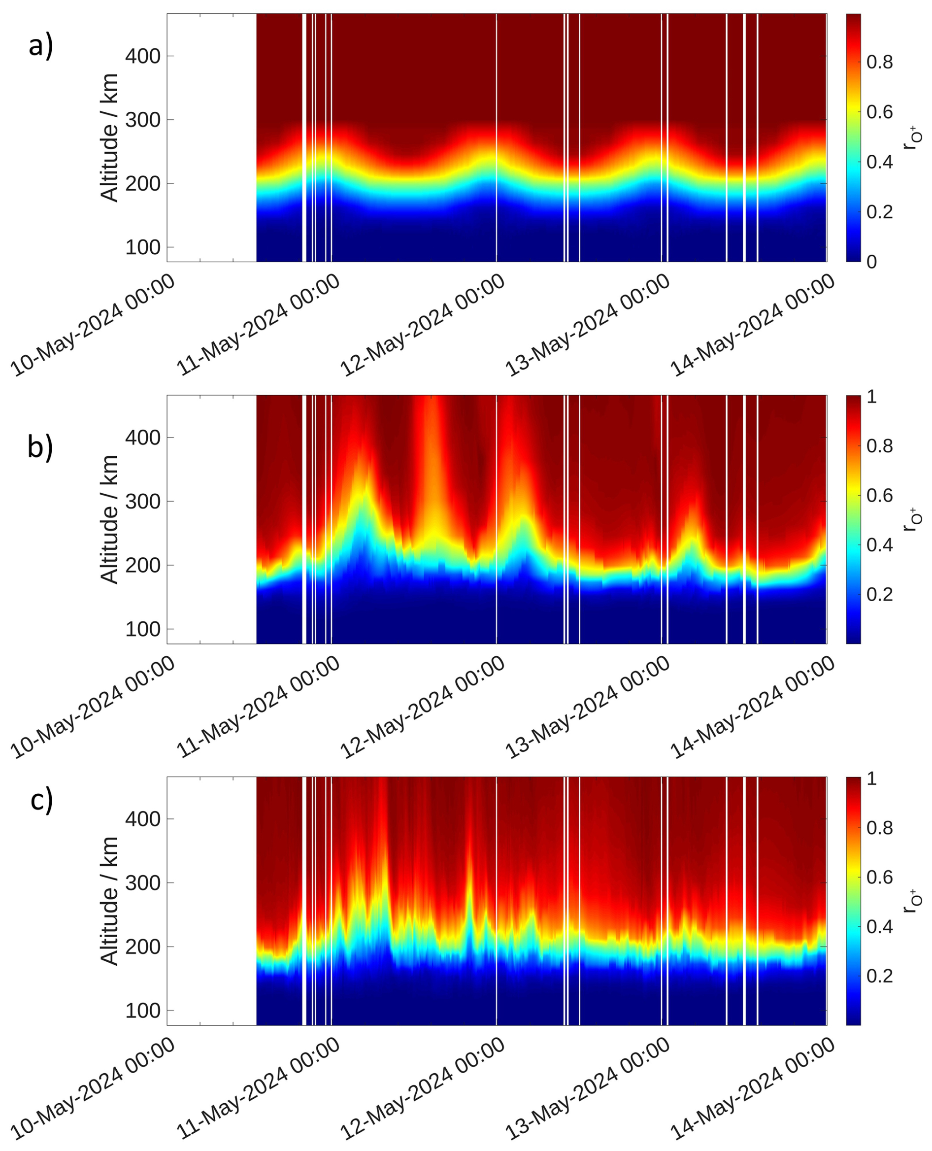
Figure 2 O⁺ ratios $r_{{\mathrm{O}}^{+}}$ given by (a) the IRI 2020 model, (b) the Heelis-driven, and (c) the AMIE-driven WACCM-X runs.

The GUSIDAP software for inferring EISCAT plasma parameters contains a subroutine ionomodel.m which, by default, calls upon the IRI 2020 model to give a priori estimates of the fitted plasma parameters as well as an a priori O⁺ ratio that is assumed as true during the fitting of plasma parameters. We adjusted this subroutine and opened a path to directly read the O⁺ ratio from the prepared WACCM-X run. The adjusted ionomodel.m routine as well as the WACCM-X data files for Heelis- and AMIE-driven model runs are provided in a software and data repository (Günzkofer et al., 2026). We would like to emphasize again that all results shown below are obtained by applying the AMIE-driven model results.

Figure 3a shows the difference of O⁺ ratio $\mathrm{\Delta }{r}_{{\mathrm{O}}^{+}}$ between WACCM-X and IRI during the May 2024 storm. Figure 3b–d show the percentage changes

$$\begin{array}{}\text{(1)}& {\displaystyle }{\displaystyle }\mathrm{d}X={\displaystyle \frac{X_{\text{reevaluation}}-X_{\text{original}}}{X_{\text{original}}}}\cdot \mathrm{100}\end{array}$$

of N_e, T_e, and T_i in the reevaluation using WACCM-X $r_{{\mathrm{O}}^{+}}$ compared to the original EISCAT parameters. It can be seen that for all three parameters dX has a negative correlation with $\mathrm{\Delta }{r}_{{\mathrm{O}}^{+}}$. While dN_e is limited to about ±10 % at maximum deviation, dT_i can reach up to ±30 % and dT_e even up to ±40 %.

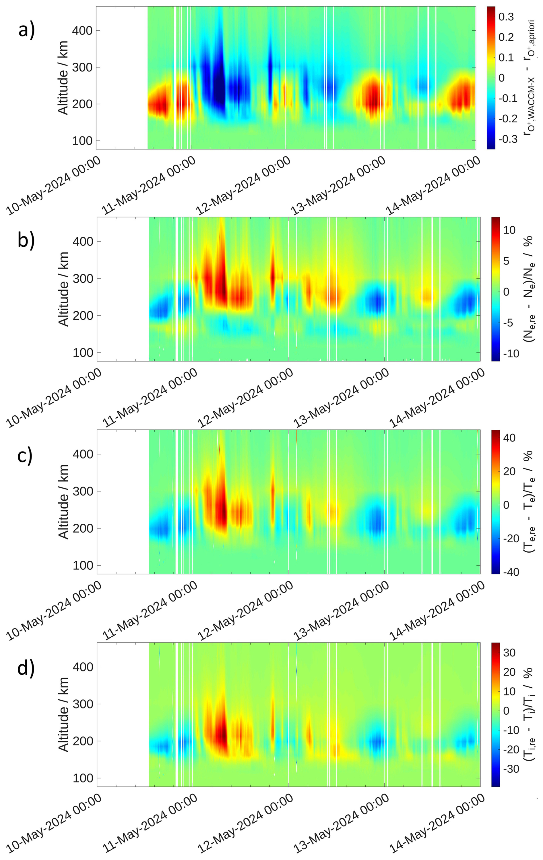
Figure 3 (a) Difference of WACCM-X O⁺ ratio compared to IRI. Applying the WACCM-X $r_{{\mathrm{O}}^{+}}$ results in reevaluated EISCAT plasma parameters N_e,re, T_e,re, and T_i,re. Panels (b)–(d) show the resulting percentage changes of these parameters.

Figure 4 illustrates the correlation of $\mathrm{\Delta }{r}_{{\mathrm{O}}^{+}}$ and dX throughout all times and altitudes shown in Fig. 3. We distinguish two altitude regimes, above and below the transition altitude z₅₀, as applied by Virtanen et al. (2021), where half of the ionospheric plasma consists of atomic oxygen ions, i.e. $r_{{\mathrm{O}}^{+}}\left(z_{\mathrm{50}}\right)=\mathrm{0.5}$. It can be seen that the percentage change between original analysis and reevaluation is strongly negatively correlated ($R<-\mathrm{0.9}$) in all cases, except for dN_e below the transition altitude. This indicates the potential to develop a simple, linear correction model which would allow to de-bias EISCAT measurements without needing to repeat the incoherent scatter analysis. For the case of dT_e above z₅₀, which has the highest correlation with $\mathrm{\Delta }{r}_{{\mathrm{O}}^{+}}$, we determine a linear function $\mathrm{d}{T}_{\mathrm{e}}=A\cdot \mathrm{\Delta }{r}_{{\mathrm{O}}^{+}}+B$, so that

$$\begin{array}{}\text{(2)}& {\displaystyle }{\displaystyle }{T}_{\mathrm{e},\text{reevaluated}}=T_{\mathrm{e},\mathrm{o}}\cdot \left({\displaystyle \frac{A\cdot \mathrm{\Delta }{r}_{{\mathrm{O}}^{+}}}{\mathrm{100}}}+{\displaystyle \frac{B}{\mathrm{100}}}+\mathrm{1}\right).\end{array}$$

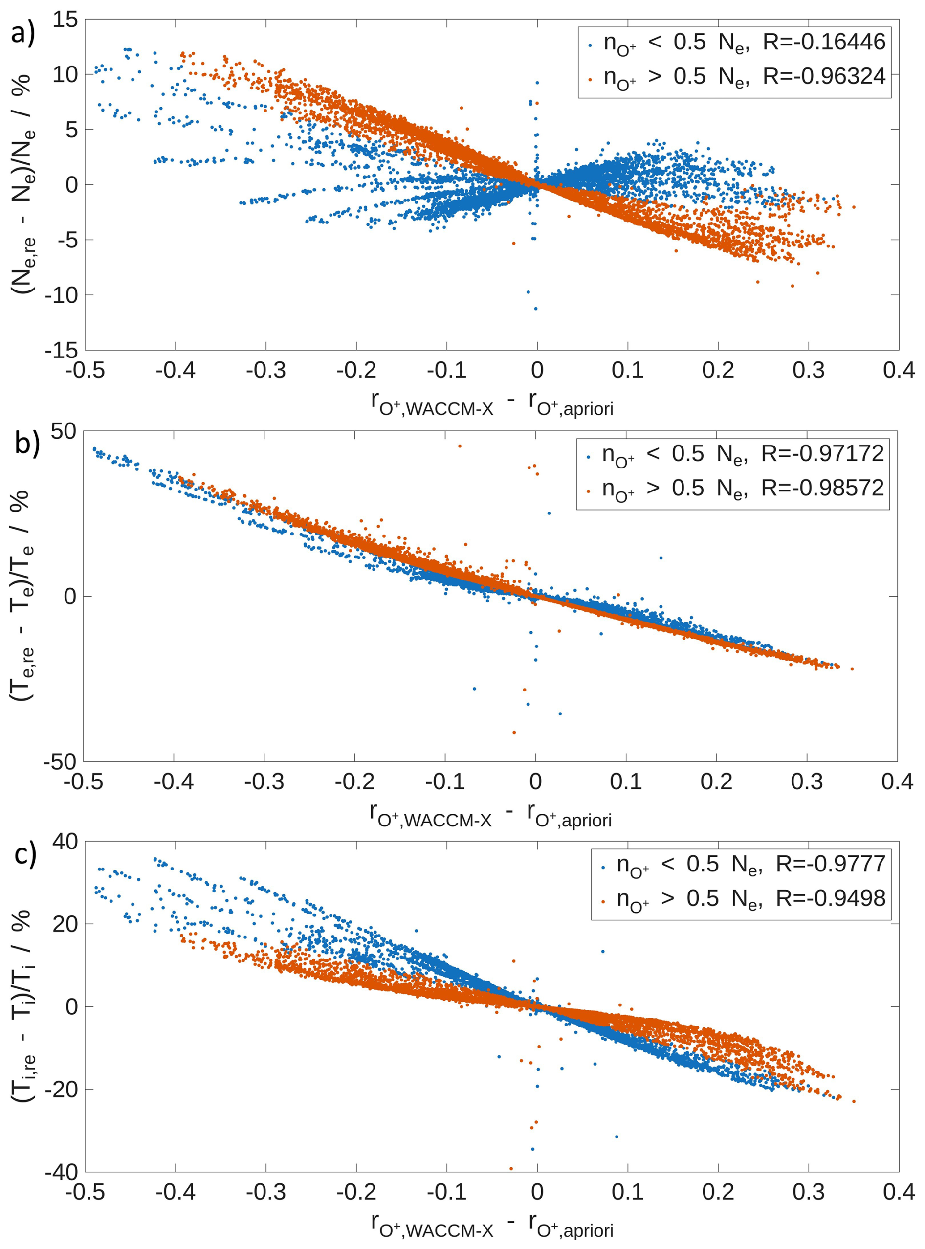
Figure 4 Correlation with $\mathrm{\Delta }{r}_{{\mathrm{O}}^{+}}$ for (a) dN_e, (b) dT_e, and (c) dT_i above and below the transition altitude.

We find that $A=-\mathrm{74.8138}$ and B=0.2261 (hence $B/\mathrm{100}\ll \mathrm{1}$ can be neglected) for this case.

However, a reliable correction model that can be applied to other EISCAT measurements would require a statistical analysis of EISCAT measurements, including quiet-time campaigns. The idea of a correction function was already suggested by Waldteufel (1971), but the significant increase in ISR measurements since then would allow for a statistically more sound evaluation. Also, non-linear relations, as already discussed by Waldteufel (1971), should be considered. The scope of this paper is the May 2024 superstorm, but the development of such a correction model might prove useful in the future.

Figure 5a–c show the analogous percentage changes of the plasma parameter uncertainties dδX. For all three parameters, the percentage change between reevaluation and the original analysis is below 10 %. However, it becomes apparent that the correlation with $\mathrm{\Delta }{r}_{{\mathrm{O}}^{+}}$ is not as straightforward as with dX in Fig. 3.

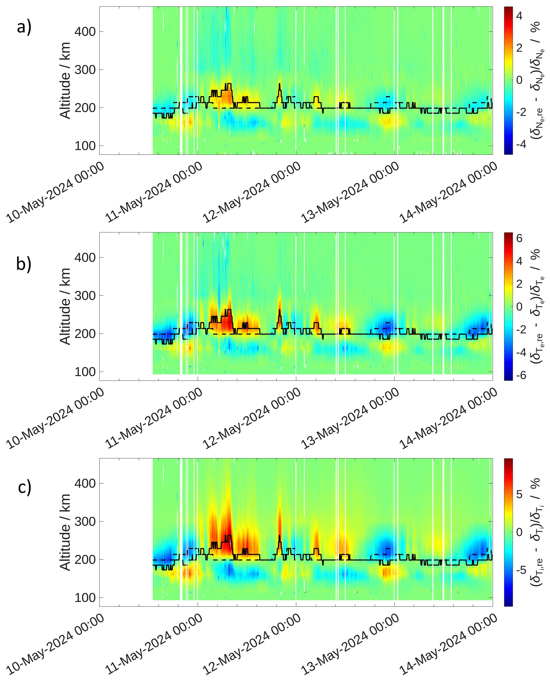
Figure 5 Percentage changes of parameter uncertainties (a) δN_e, (b) δT_e, and (c) δT_i. Transition altitudes of $r_{{\mathrm{O}}^{+}}=\mathrm{0.5}$ are shown as solid (WACCM-X) and dashed (IRI) lines.

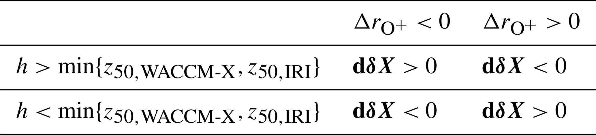
In Fig. 5, the transition altitudes given by the IRI and WACCM-X models, interpolated to EISCAT measurement altitudes, are shown as solid (WACCM-X) and dashed (IRI) lines. The percentage change of the parameter uncertainties has an opposite sign above, and below the smaller of the two compared transition altitudes, i.e. it depends on whether the altitude h is larger or smaller than $\text{min}\mathit{\{}{z}_{\mathrm{50},\text{WACCM-X}},z_{\mathrm{50},\text{IRI}}\mathit{\}}$. Table 1 summarizes the relations of $\mathrm{\Delta }{r}_{{\mathrm{O}}^{+}}$, h, and dδX. To our understanding, the origin of the relations in Table 1 is rather a mathematical consequence of the incoherent scatter analysis than an actual physical process, though no evidence can be provided.

Table 1 Whether the plasma parameter uncertainties increase or decrease due to the reevaluation depends on the sign of $\mathrm{\Delta }{r}_{{\mathrm{O}}^{+}}$ and on the altitude of the lower model z₅₀.

To obtain an impression of how the impact of the reevaluation, Figs. 6 and 7 show the vertical profiles of N_e, T_e, and T_i for 11 May 08:00 UTC and 12 May 22:10 UTC, which are the times of minimum/maximum $\mathrm{\Delta }{r}_{{\mathrm{O}}^{+}}$ respectively.

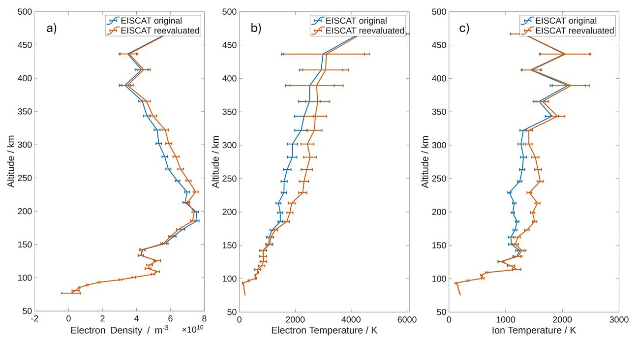
Figure 6 Vertical profiles of (a) N_e, (b) T_e, and (c) T_i from the original EISCAT analysis and the reevaluation at 08:00 UTC on 11 May 2024.

Figure 7 Same as Fig. 6 but for 22:10 UTC on 12 May 2024.

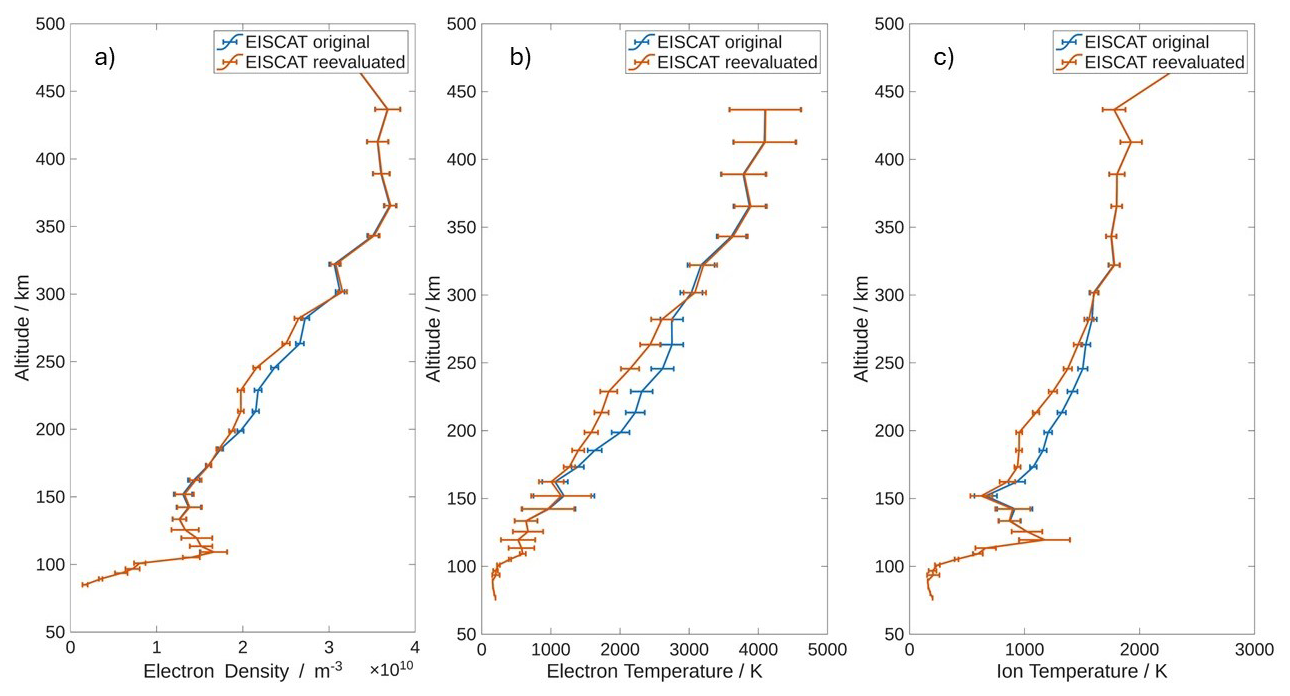
It can be seen that the deviation of the original and reevaluated profiles is mostly larger than the uncertainty range at around 200–300 km altitude. This demonstrates the usefulness of such a reevaluation, especially for studies investigating plasma temperatures.

4 Discussion

This section discusses alternative approaches to constrain/determine the O⁺ ratio before or during the analysis process, in addition to the default GUSIDAP analysis, using IRI $r_{{\mathrm{O}}^{+}}$, and the WACCM-X-based reevaluation presented in this paper. The advantages and disadvantages of each method will be compared.

4.1 Direct fitting of O⁺ ratios

The GUISDAP software package allows for determining $r_{{\mathrm{O}}^{+}}$ during the analysis process without constraining it to the a priori profile. However, this results in a very noisy $r_{{\mathrm{O}}^{+}}$, as shown in Fig. 8, and consequently large uncertainties of all inferred parameters.

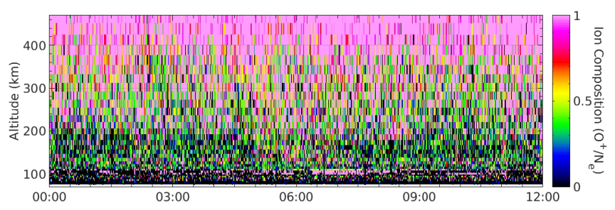
Figure 8 GUISDAP fit of O⁺ ratio without constraining any other parameters on 12 May 2024 (00:00–12:00 UTC).

This issue has been previously discussed in numerous publications (see Blelly et al., 2010; Zettergren et al., 2011, and references therein), and alternative approaches have been discussed. Introducing a correction function, as suggested by Waldteufel (1971) and in Eq. (2) has the advantage of not requiring a time-consuming reevaluation of the incoherent scatter measurements. The problem with this approach is that $r_{{\mathrm{O}}^{+}}$ is still assumed to be known somehow (in our case, from AMIE/WACCM-X instead of IRI).

Blelly et al. (2010) suggested a complete reparameterization of the incoherent scatter analysis. This method allows inferring the standard ISR plasma parameters as well as $r_{{\mathrm{O}}^{+}}$ from the incoherent scatter spectrum. However, multiple assumptions about the shape of $r_{{\mathrm{O}}^{+}}$ and the ionospheric temperatures are applied to obtain the additional parameter. Oliver (1975) derived an altitude profile for the O⁺ ratio

$$\begin{array}{}\text{(3)}& {\displaystyle }{\displaystyle }{r}_{{\mathrm{O}}^{+}}\left(h\right)={\displaystyle \frac{\mathrm{2}}{\mathrm{1}+\sqrt{\mathrm{1}+\exp \left(-\frac{h-z_{\mathrm{50}}}{H}\right)}}}\end{array}$$

based on the transition altitude z₅₀ and a scale height parameter H for the thickness of the transition. Zettergren et al. (2011) applied Eq. (3) with a constant H for further simplification they deemed justified (Zettergren et al., 2010) while Blelly et al. (2010) implemented an asymmetric profile with different H⁺ and H⁻ above and below z₅₀.

The above-described approaches provide self-consistent measurements of the ionospheric composition together with the standard ISR plasma parameters. However, the required modification of the incoherent scatter analysis limits their applicability, and the applied assumptions on the $r_{{\mathrm{O}}^{+}}$ profile and the ionospheric temperatures provide additional uncertainty (e.g. Eq. 3 was specifically derived for mid-latitudes). The method suggested in this paper, together with the correction-function approach from Waldteufel (1971), is easily applicable, and the only, though major, assumption is the reliability of WACCM-X ion compositions. Its main use can therefore be seen as a “quick correction” for cases where IRI ion composition is presumably erroneous (e.g. during strong storm events).

4.2 Bayesian Fitting Module

Another possible approach is the Bayesian Filtering Module (BAFIM) developed by Virtanen et al. (2021). BAFIM is a full-profile fitting technique that allows inferring the four standard ISR plasma parameters at high time and altitude resolution from a multi-step fitting process. Since the full-profile fitting approach, other than the standard gate-by-gate analysis, allows for enforcing certain conditions on the parameter profiles, the ion composition can be fitted as an additional fifth parameter. The five-parameter BAFIM analysis in Virtanen et al. (2021) was able to eliminate the artificial temperature maximum in the F1 region that is often observed in ISR measurements under erroneous $r_{{\mathrm{O}}^{+}}$ assumptions (Günzkofer et al., 2025b). In Virtanen et al. (2024), the BAFIM was coupled to an ion chemistry model (Richards et al., 2010; Reimer et al., 2021), providing even more reliable ion composition fits in an approach similar to the one applied in the AMISR radars (Richards et al., 2010). The iterative fit of plasma parameters and ion composition ensures that the result of the fit is reasonable from a chemistry point of view. Hence, that technique is also suitable for rapid changes in ion temperature and composition, which typically occur during active geomagnetic conditions, such as substorms and storms.

For the May 2024 storm, Cai et al. (2026) recently showed BAFIM analyzed EISCAT measurements (see their Fig. 3). It can be seen that the BAFIM fitted O⁺ ratios evolve, similar to the AMIE-driven WACCM-X results. Assuming the BAFIM results as ground-truth, this confirms our initial assumption that under storm conditions, physics-based T-I models can capture the ion composition better than empirical models. The Heelis-driven WACCM-X run shows a somewhat different evolution of O⁺ ratio over Svalbard, but still seems to capture the storm better than IRI. It should be noted that the transition altitude z₅₀ of the BAFIM fitted ion composition can be at altitudes >300 km. Both WACCM-X runs show consistently higher O⁺ ratios, equivalent to lower transition altitudes than the BAFIM fit. It is known that WACCM-X generally overestimates $\sum \mathrm{O}/{\mathrm{N}}_{\mathrm{2}}$ ratios (Liu et al., 2023). Since the dominant production process of O⁺ is photoionization of atomic oxygen, an overestimation of O⁺ ratio can therefore be expected.

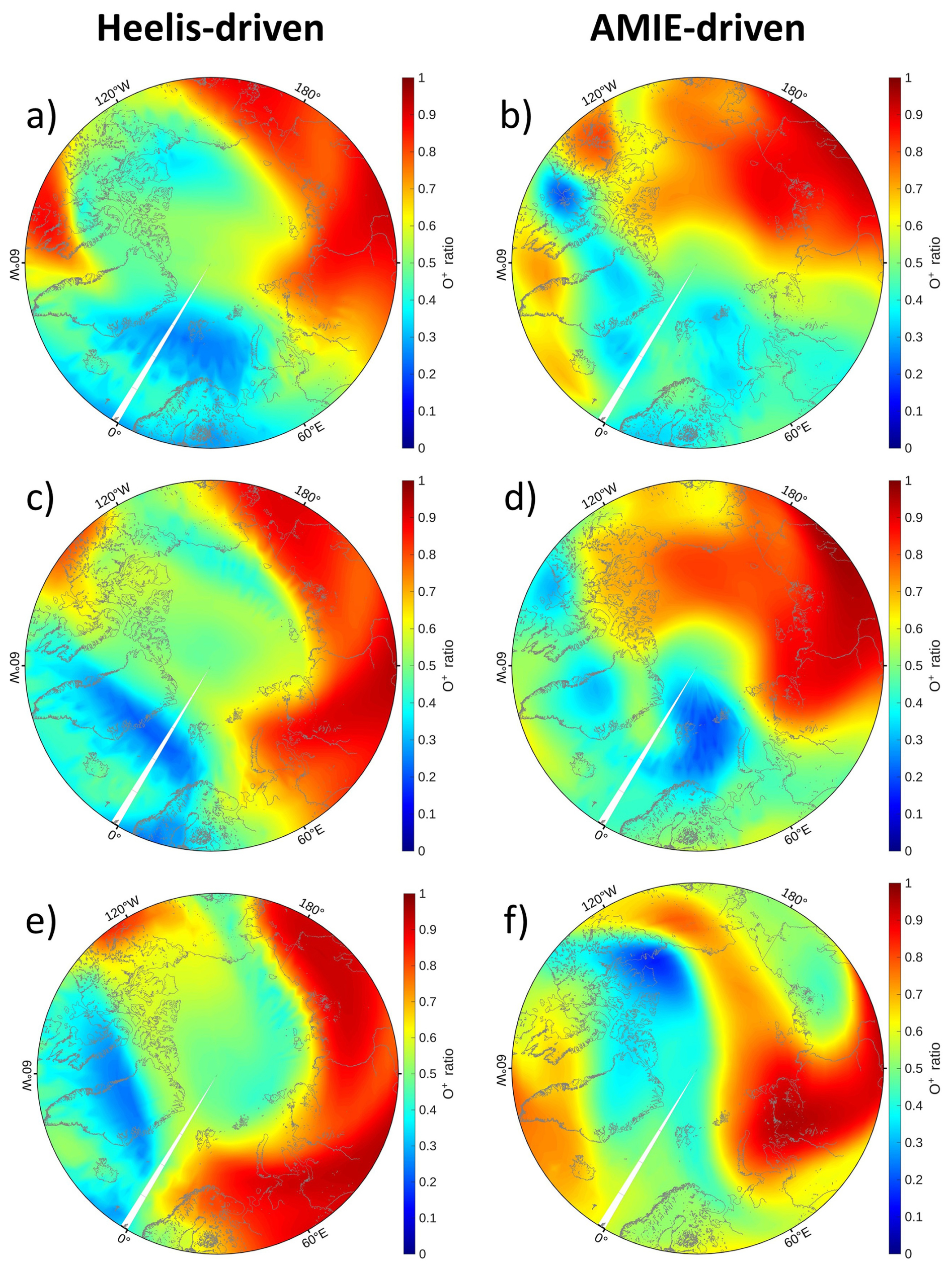
Figure 9 WACCM-X distributions of O⁺ ratio over the arctic cap at 230 km altitude at (a, b) 04:00 UTC, (c, d) 06:00 UTC, and (e, f) 08:00 UTC on 11 May 2024. The left column shows Heelis-driven and the right column shows AMIE-driven model results. We leverage the M_Map software package (Pawlowicz, 2020) for plotting.

The Bayesian Filtering Module, in combination with the GUISDAP software, provides the presumably most reliable method for inferring EISCAT plasma parameters and “correct” ion compositions. Since the main challenge is the sparse availability of ion composition measurements in the F1 region, a thorough validation is difficult. An additional problem of full-profile techniques is the large computational weight, though BAFIM avoids this issue by partially applying gate-by-gate analysis (Virtanen et al., 2021). Nevertheless, many users of EISCAT measurements do not conduct the incoherent scatter analysis themselves but rely on data products provided by the EISCAT database. Especially for these users, a simple and quick, if less accurate, correction function, as suggested in this paper, is presumably more applicable. However, the accuracy of physics-based model ion compositions, especially for empirical convection forcing (see Sect. 4.3) needs to be investigated. It needs to be determined under what geomagnetic conditions physics-based ion compositions outperform empirical models before a correction model can be derived from a statistically representative database of EISCAT measurements and WACCM-X simulations For the required evaluation of model O⁺ ratios, BAFIM will be highly valuable as an independent reference.

4.3 Model variability of $r_{{\mathrm{O}}^{+}}$

As previously discussed, the main issue of the proposed method is that it still relies on model O⁺ ratios. As argued in the previous Section, the AMIE-driven WACCM-X run captures the general dynamics of the O⁺ ratio, assuming the BAFIM results as ground-truth, significantly better than IRI during storm times.

In Fig. 2b and c, the different temporal scales of the Heelis and AMIE convection models can be seen. While the investigated WACCM-X runs all apply a five-minute output cadence, the Heelis model is driven by the 3-hourly Kp index, and hence strong variability of $r_{{\mathrm{O}}^{+}}$ occurs only on temporal scales >3 h in Fig. 2b. The data assimilative AMIE model can produce ionospheric variability on a temporal scale of a few minutes and is therefore capable of capturing storm dynamics better than Heelis (Günzkofer et al., 2025a). Since WACCM-X long-runs mainly apply the Heelis convection model, e.g. Brown et al. (2026), the development of an empirical correction model will need to consider the missing temporal-scales of Heelis-driven WACCM-X ionosphere dynamics.

In addition to temporal scales, the horizontal variability of different forcing models needs to be considered. Figure 9 shows the O⁺ ratios given by Heelis- and AMIE-driven WACCM-X runs over the northern polar cap at 230 km altitude. Both models show a distinct patch of low O⁺ ratio in the vicinity of Svalbard that intensifies between 06:00–08:00 UTC on 11 May 2024. However, in the Heelis-driven run, this patch appears to remain fixed in local time, whereas it is convected across the polar cap in the AMIE-driven run. This results in a different horizontal distribution of $r_{{\mathrm{O}}^{+}}$ at 10 UTC (Fig. 9e and f in both model runs. Before a correction model based on the correlations identified in Sect. 3 can be developed, the variability of O⁺ in Heelis-driven model runs needs to be better understood, and it needs to be assessed under what conditions the physics-based model can be assumed to give more accurate a priori conditions than the empirical IRI model.

5 Conclusions and Outlook

A reevaluation of EISCAT plasma parameters during the May 2024 geomagnetic storm was conducted, assuming O⁺ ratios from an AMIE-driven SD-WACCM-X run. We showed that under extreme storm conditions, the EISCAT electron density measurements deviate up to 15 % compared to the standard analysis assuming IRI O⁺ ratios. Electron and ion temperatures were shown to deviate even stronger, up to 40 % and 30 %, respectively. We showed a very high linear correlation of electron temperature deviations and $r_{{\mathrm{O}}^{+}}$ in the applied a priori models, opening the possibility to introduce a simple correction function. The uncertainties in the plasma parameters were impacted by the reevaluation, increasing by about 5 %–10 %. However, whether the uncertainty is increased or decreased due to the reevaluation depends on the transition altitudes of the two a priori models. However, the deviations of F1 region plasma parameters between the original analysis and reevaluation are notably larger than the uncertainty range.

As discussed in Sect. 4, the main advantage of an ISR measurement reevaluation based on the ion composition given by a physics-based thermosphere-ionosphere model is the possibility to extend the method into a correction model. Due to the limited availability of AMIE results coinciding with EISCAT measurements, a correction model would have to be based on standard high-latitude drivers of WACCM-X, i.e. the Heelis and Weimer empirical convection models. Existing WACCM-X long-runs, such as Brown et al. (2026), can be applied. Such a correction model would be quickly and easily applicable to all researchers, regardless of their proficiency with incoherent scatter analysis software. However, extended studies including ISR campaigns during different levels of geomagnetic activity are required to verify the possibility of inferring a correction model, and it needs to be determined under what conditions physics-based models actually capture the ionosphere composition better than empirical models.