Data reduction of incoherent scatter plasma line parameters

In the ionosphere, a sustained population of suprathermal electrons arises due to photoionization or electron precipitation. The presence of such a population enhances the scattered power in the plasma line spectrum, thus making it possible to detect them. Plasma line measurements improve the accuracy of electron density and temperature estimates. We investigate plasma line enhancements in EISCAT Tromsø UHF radar observations, using two image processing methodologies for detection: a supervised image morphological processing technique and an unsupervised connected component analysis. The supervised methodology detects more plasma lines, demonstrating higher sensitivity. We determine the times and altitudes with enhancements and model the spectrum with a Gaussian function. The radar beam points in the field-aligned direction for 25 % of the total observational time, is directed east for another 25 % and is oriented in the vertical direction for the remaining 50 %. Plasma lines are detected 26 % of the time when the radar is pointed in the field-aligned direction, 5 % of the time in the east direction and 5 % of the time in the vertical direction. Most plasma lines are detected around the F-region altitude where the electron density is maximum, typically between 230–260 km, with a simultaneous increase in the electron density estimates from the ion line. Plasma line intensity is maximum around noon. It decreases as the aspect angle increases. Both detection methodologies' advantages and disadvantages are discussed, and plasma line intensity variations are analyzed as a function of altitude, aspect angle and phase energy.

1 Introduction

Powerful electromagnetic pulses are transmitted by incoherent scatter radars (ISRs) into the ionosphere, causing electrons to oscillate and re-radiate along the radar scattering wave vector. The scattering wave vector depends on the radar operating frequency and geometry. The scattered signal is collected by the radar and analyzed as a power spectrum (Dougherty and Farley, 1960). ISRs probe the ionospheric plasma at a wavelength much greater than the Debye length, λ_D i.e.

$$\begin{array}{}\text{(1)}& \mathit{\alpha }={\displaystyle \frac{\mathrm{1}}{k_{\mathrm{s}}{\mathit{\lambda }}_{\mathrm{D}}}}\gg \mathrm{1},\end{array}$$

where $k_{\mathrm{s}}=\mathrm{2}\mathit{\pi }/{\mathit{\lambda }}_{\mathrm{s}}$, k_s and λ_s are the scattering wavenumber and wavelength, respectively. The electron Debye length is defined as ${\mathit{\lambda }}_{\mathrm{D}}=\sqrt{{\mathit{ϵ}}_{\mathrm{0}}{k}_{\mathrm{B}}{T}_{\mathrm{e}}/n_{\mathrm{e}}{e}^{\mathrm{2}}}$ where ϵ₀ is the permittivity of free space, k_B is the Boltzmann constant, T_e is the electron temperature, n_e is the electron density and e is the electron charge. ISRs provide valuable information about the collective interactions in the plasma. Most of the scattered power is present at pairs of frequencies corresponding to the natural electrostatic modes of the plasma, where the resonance condition of the magnetized plasmas is satisfied (Evans, 1969). The Doppler shift of each frequency can be either positive, indicating a wave travelling towards the radar, or negative, signifying a wave travelling away along the scattering direction. These resonant frequency pairs are classified as ion lines and plasma lines, corresponding to ion acoustic waves and Langmuir waves, respectively (Akbari et al., 2017).

Most of the scattered power is contained within the ion lines. The integrated power of the ion line in thermal equilibrium is given by Bauer (1975) and Fredriksen et al. (1992)

$$\begin{array}{}\text{(2)}& I_{\mathrm{i}}={\displaystyle \frac{{\mathit{\alpha }}^{\mathrm{4}}}{\left(\mathrm{1}+{\mathit{\alpha }}^{\mathrm{2}}\right)\left(\mathrm{1}+{\mathit{\alpha }}^{\mathrm{2}}+{\mathit{\alpha }}^{\mathrm{2}}{T}_{\mathrm{e}}/T_{\mathrm{i}}\right)}},\end{array}$$

where T_i is the ion temperature. The ion line spectrum is fitted to a model power spectrum, under the assumption of scatter from a uniform plasma in thermal equilibrium i.e. the electron and ion velocity distributions are Maxwellian. The three-dimensional isotropic Maxwellian velocity distribution for species s is given by

$$\begin{array}{}\text{(3)}& f_{\mathrm{s}}\left(\mathit{v}\right)={\left({\displaystyle \frac{m_{\mathrm{s}}}{\mathrm{2}\mathit{\pi }{k}_{\mathrm{B}}{T}_{\mathrm{s}}}}\right)}^{\frac{\mathrm{3}}{\mathrm{2}}}\exp \left(-{\displaystyle \frac{m_{\mathrm{s}}(\mathit{v}-{\mathit{u}}_{\mathrm{s}}{)}^{\mathrm{2}}}{\mathrm{2}{k}_{\mathrm{B}}{T}_{\mathrm{s}}}}\right),\end{array}$$

where m_s is the mass, T_s the temperature, and u_s the bulk drift velocity of species s (either electron e or ion i). The ionospheric plasma parameters $n_{\mathrm{e}},T_{\mathrm{e}},T_{\mathrm{i}}$ and u_i are estimated from the ion line for each range gate. In this case, the range gate is equal to the spatial resolution of the analysis. These parameters characterize the uniform background ionospheric plasma along the direction of the scattering wavevector (Kudeki and Milla, 2011). For a thermal plasma, the integrated power in one plasma line is written as:

$$\begin{array}{}\text{(4)}& I_{\mathrm{p}}={\displaystyle \frac{\mathrm{1}}{\mathrm{2}{\mathit{\alpha }}^{\mathrm{2}}}}.\end{array}$$

when the condition Eq. (1) is satisfied, then the ratio of the integrated power in the plasma line (I_p) and the ion line (I_i) is given by Bauer (1975)

$$\begin{array}{}\text{(5)}& {\displaystyle \frac{I_{\mathrm{p}}}{I_{\mathrm{i}}}}\approx {\displaystyle \frac{\mathrm{1}}{\mathrm{2}{\mathit{\alpha }}^{\mathrm{2}}}}\left(\mathrm{1}+{\displaystyle \frac{T_{\mathrm{e}}}{T_{\mathrm{i}}}}\right).\end{array}$$

This implies that plasma lines generally contain less power than the ion lines, as seen in Eq. (5), and are difficult to observe in uniform plasmas in thermal equilibrium. However, photoionization or auroral precipitation can generate a suprathermal population and the power in the plasma line spectra can be enhanced (Perkins and Salpeter, 1965). Plasma lines may also be strongly enhanced by plasma instabilities and Langmuir turbulence. Such processes can lead to intensities several orders of magnitude above the thermal level, and have been studied both theoretically and observationally. For example, Guio and Forme (2006) presented a numerical study of Langmuir turbulence driven by low-energy electron beams, while Isham et al. (2012) reported the first direct evidence of naturally occurring cavitating Langmuir turbulence in the ionosphere. A comprehensive review of these processes is given by Akbari et al. (2017).

Plasma line measurement enables the study of several properties that are not directly available with only the measurement of the ion lines. For example, plasma lines allow for the analysis of fine structures in suprathermal electron velocity distribution at velocities imposed by the plasma line frequency and the radar frequency (Guio and Lilensten, 1999). Electron density and temperature estimates are also improved by plasma lines (Nicolls et al., 2006). Plasma line asymmetry can be used to measure electron drift velocity and electron density, which, together with ion drift velocity, provide an estimate of the ionospheric current (Guio et al., 1996). Plasma line measurements facilitate the determination of additional parameters, like ion composition (Bjørnå and Kirkwood, 1988; Fredriksen et al., 1989) and ion-neutral collision frequency (Bjørnå, 1989) by providing extra constraints, reducing ambiguity between parameters.

Plasma lines have been the subject of numerous studies. Investigations of plasma lines along the magnetic field at high latitudes have encompassed experimental studies (Guio et al., 1996), theoretical modelling (Nilsson et al., 1996) as well as comparing experimental data with theoretical modelling (Guio and Lilensten, 1999). Plasma line parameters at oblique angles to the magnetic field have also been explored through experimental measurements at low latitudes (Djuth et al., 2018) and comparative studies combining theoretical models with experimental data at both low latitudes (Fremouw et al., 1969; Longley et al., 2021) and high latitudes (Fredriksen et al., 1992; Kirkwood et al., 1995). Kirkwood et al. (1995) focused exclusively on plasma lines in the E-region, while Fredriksen et al. (1992) considered plasma lines in the F-region as well. However, these studies do not address high-latitude F-region plasma line intensity measurements as a function of phase energy at low aspect angles, a gap we aim to fill.

In Sect. 2 we present a description of the EISCAT UHF radar experimental setup and IP2 scanning technique used to collect the data presented here. Section 3 covers the general methodologies for supervised and unsupervised detection of plasma lines, parameter extraction using Gaussian model fitting and intensity derivation. In Sect. 4, we summarize the main findings from applying these methodologies to ISR data collected with the EISCAT UHF radar in Tromsø between 07:00–15:00 UT from 26 to 31 January 2022. Finally, Sect. 5 discusses the advantages and disadvantages of the supervised and unsupervised detection methodologies, examines plasma line intensity variations as a function of time, altitude, phase energy, and the aspect angle between the magnetic field and the scattering wavevector, and suggests areas for future research.

2 Experiment

The data analyzed in this study were collected with the EISCAT UHF radar in a scanning sequence as part of a common programme experiment known as the IP2 or CP2 experiment. The IP2 scan consists of a beam-swing sequence where the antenna points in three directions in a short cycle. The details of the radar scan sequence are described in Table 1. It takes 15 s for the radar to manoeuvre between pointing directions, and therefore, the radar scan cycle duration is 4 min. The scattering wavevector is the difference between the received and transmitted wavevector ${\mathit{k}}_{\mathrm{s}}={\mathit{k}}_{\mathrm{r}}-{\mathit{k}}_{\mathrm{t}}$. For a monostatic radar, i.e. a radar with same antenna to transmit and receive and transmitting and receiving at the same operating frequency f_radar, k_t and k_r have the same magnitude $k_{\mathrm{t}}=k_{\mathrm{r}}=\mathrm{2}\mathit{\pi }{f}_{\text{radar}}/c$ with c the speed of light in vacuum and the scattering wavevector is ${\mathit{k}}_{\mathrm{s}}=-\mathrm{2}{\mathit{k}}_{\mathrm{t}}$ with wavenumber $k_{\mathrm{s}}=\mathrm{4}\mathit{\pi }{f}_{\text{radar}}/c$. For the EISCAT UHF radar, $k_{\mathrm{s}}=\mathrm{39}{\mathrm{m}}^{-\mathrm{1}}$.

Table 1 Radar scan direction and angles.

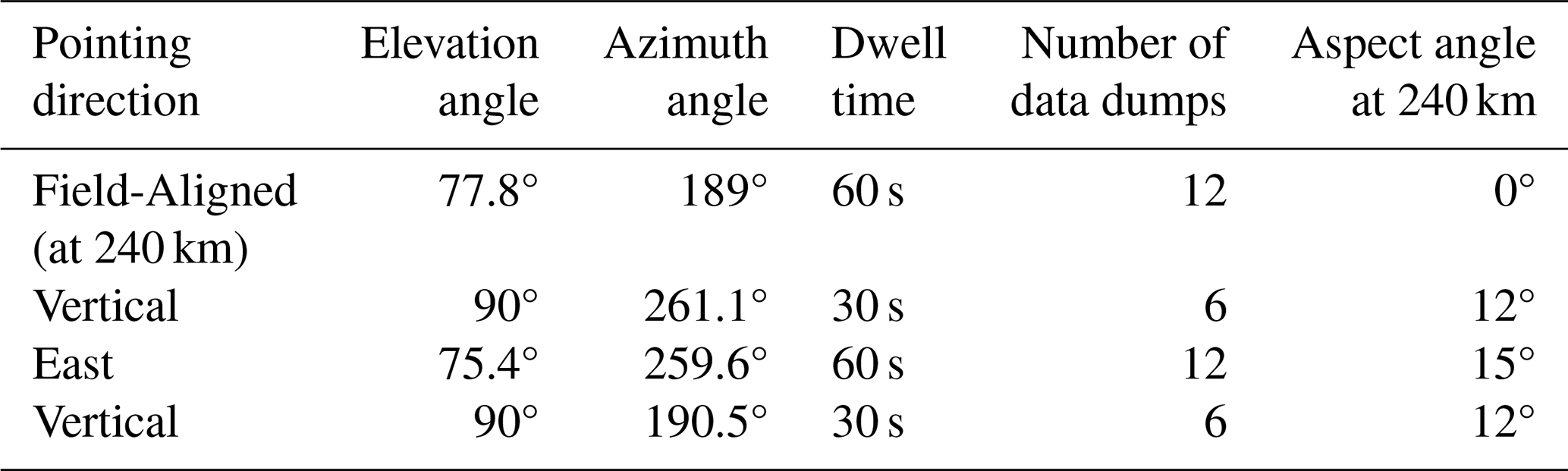
The radar has a transmitter frequency of 927 MHz (wavelength λ=32.2 cm), a peak power of 1 MW and a 11 % duty cycle. The experiment uses a 32 bit alternating code transmitter scheme with a baud length of 20 µs. Each code consists of 64 subcycles of duration 5.58 ms, resulting in a total cycle duration of 0.357 s. Measurements have a pre-integration time of 5 s, with a total of 14 cycles included in each data dump. It is assumed that the ionosphere remains stationary throughout this time resolution.

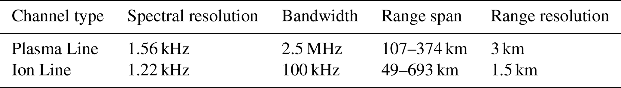
The raw data collected by the radar consists of the autocorrelation function (ACF) evaluated at discrete time lags (Lehtinen and Häggström, 1987). Plasma line ACFs are sampled with a lag increment of 0.4 µs, and the maximum lag is 320 µs, resulting in a total of 800 lags. The power spectrum is derived by taking the Fourier transform of the ACF. The resulting frequency resolution of the power spectrum is 1.56 kHz and a bandwidth of 2.5 MHz. The spectra consist mostly of white noise, with the possibility of a narrow-banded plasma line signal being present. Plasma line data from two downshifted receiver bands (between −5.25 and −2.75 MHz, and between −7.65 and −5.15 MHz) were analyzed. Data were examined from 07:00 to 15:00 UT every day between 26–31 January 2022. The spectral and range characteristics of the ion line and plasma line channels are given in Table 2.

Table 2 Characteristics of plasma and ion line channels.

3 Methodology

3.1 Derivation of plasma line spectra

We used GUISDAP (Lehtinen and Huuskonen, 1996) for analyzing ion lines and extended its capabilities to assess plasma lines. The analysis was performed on the collected data from the EISCAT UHF radar. The data were integrated over each position's dwell time, followed by background subtraction and calibration. The power spectra were obtained by taking a Fourier transform of the ACF. At this stage, we have, for each time, two-dimensional data depicting the plasma line antenna temperature as a function of frequency and altitude as depicted in the upper left plots in Figs. 1 and 2.

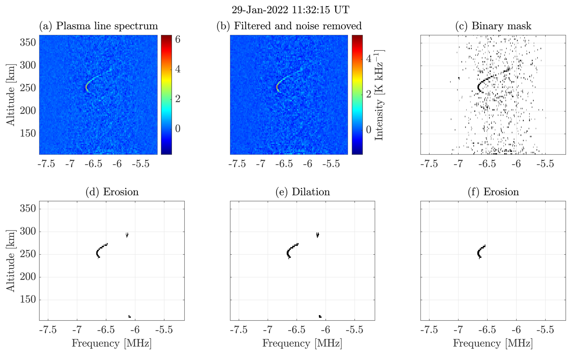
Figure 1 Image morphological processing steps for plasma line detection: (a) plasma line spectra as a function of altitude and frequency with 60 s integration time and 0° aspect angle, (b) median filtering (3 point frequency width) and background noise removal, (c) binary mask creation (threshold at 3.98×MAD), (d) removal of regions with less than 16 connected points, (e) convolution with the rectangular kernel (one range gate × three frequency bins), and (f) removal of regions with less than 47 connected points.

Figure 2 Plasma line detection using connected component analysis: (a) and (b) are the same as in Fig. 1, (c) threshold $\mathrm{3.4}\times {\mathrm{10}}^{-\mathrm{3}}\mathrm{K}{\mathrm{kHz}}^{-\mathrm{1}}$ on (b) to convert to binary image, (d) largest connected component identifying the plasma line.

3.2 Plasma line detection

To identify times and altitudes with enhanced plasma lines, we implemented two methodologies: a supervised one based on image morphological processing and an unsupervised one based on connected components. Both methodologies begin with the same initial steps: median filtering of the spectra and noise removal, as described by Ivchenko et al. (2017). A median filter of size 1×3 was applied, where 1 and 3 are the number of points in the range and frequency dimensions, respectively. Noise and clutter were removed using the methodology described in Ivchenko et al. (2017). The spectra obtained after filtering and removing noise are shown in the upper middle plot of Fig. 1 and the upper right plot of Fig. 2.

Additionally, both methodologies use the median absolute deviation estimator, denoted MAD, to assess the dispersion in the spectra and set thresholds for detecting points with high power in the spectral image. Given a sample dataset, x, with a median value of $\stackrel{\mathrm{̃}}{x}=\text{median}\left(x\right)$, the MAD estimator is defined as Wilrich (2007):

$$\begin{array}{}\text{(6)}& \text{MAD}=\text{median}\left(\right|x-\stackrel{\mathrm{̃}}{x}\left|\right).\end{array}$$

For the examples shown in Figs. 1 and 2, the MAD for the filtered and noise-removed image is calculated to be $\mathrm{1.2}\times {\mathrm{10}}^{-\mathrm{4}}\mathrm{K}{\mathrm{kHz}}^{-\mathrm{1}}$. A discussion of both methodologies follows below.

3.2.1 Supervised methodology: image morphological processing

We implemented the technique proposed by Ivchenko et al. (2017) but with different parameters for thresholding and image morphological processing tailored to each channel for detecting enhanced profile points. We calibrated the image morphological processing parameters through iterative manual adjustment, examining the spectra to avoid false positives.

For the first downshifted channel (−5.25 to −2.75 MHz), a threshold of 3.95×MAD was set to obtain a binary mask. Regions with fewer than 10 connected points were then eroded. This was followed by dilation using a structuring element sized 1×3, where 1 corresponds to the range (no dilation) and the frequency (dilation across 3 points). Subsequently, regions with less than 45 connected points were removed to yield the final mask containing the plasma line signal.

In the case of the second downshifted channel (−7.65 to −5.15 MHz), a threshold of 3.98×MAD was applied. This was followed by the erosion of areas containing fewer than 16 connected points, dilation using the same 1×3 structuring element as in the first downshifted channel, and a subsequent erosion targeting areas with less than 47 connected points.

In our study, the values for binary thresholding, erosion, and dilation are smaller in comparison to those used by Ivchenko et al. (2017). This difference is due to the signal-to-noise ratios (SNR) with EISCAT UHF measurements having higher SNR than the EISCAT Svalbard radar, as highlighted by Nilsson et al. (1996).

3.2.2 Unsupervised methodology: connected component analysis

MAD approximates the width w of the 50 %-interval around the median $\stackrel{\mathrm{̃}}{x}$ of the distribution of x as $P(\left|x-\stackrel{\mathrm{̃}}{x}\right|\le w)=\mathrm{0.5}$. Under the assumption of normality in the data distribution, w can be expressed as:

$$\begin{array}{}\text{(7)}& w=z_{\mathrm{0.75}}\mathit{\sigma }=\mathrm{0.6745}\mathit{\sigma },\end{array}$$

with z_0.75 being the 75 %-quantile of the standard normal distribution and σ is the standard deviation. However, this estimator is inherently biased and tends to underestimate variability. To obtain an unbiased estimate under normality, we apply a bias correction to the MAD estimator. The bias-corrected median absolution deviation is Daszykowski et al. (2007)

$$\begin{array}{}\text{(8)}& {\mathit{\sigma }}_{\text{MAD}}=\text{MAD}/\mathrm{0.6745}=\mathrm{1.4826}\cdot \text{MAD}.\end{array}$$

This correction gives an unbiased estimator with an asymptotic efficiency of 36.7 % and an asymptotic breakdown point of 50 %, meaning it remains reliable even when up to 50 % of the data are outliers.

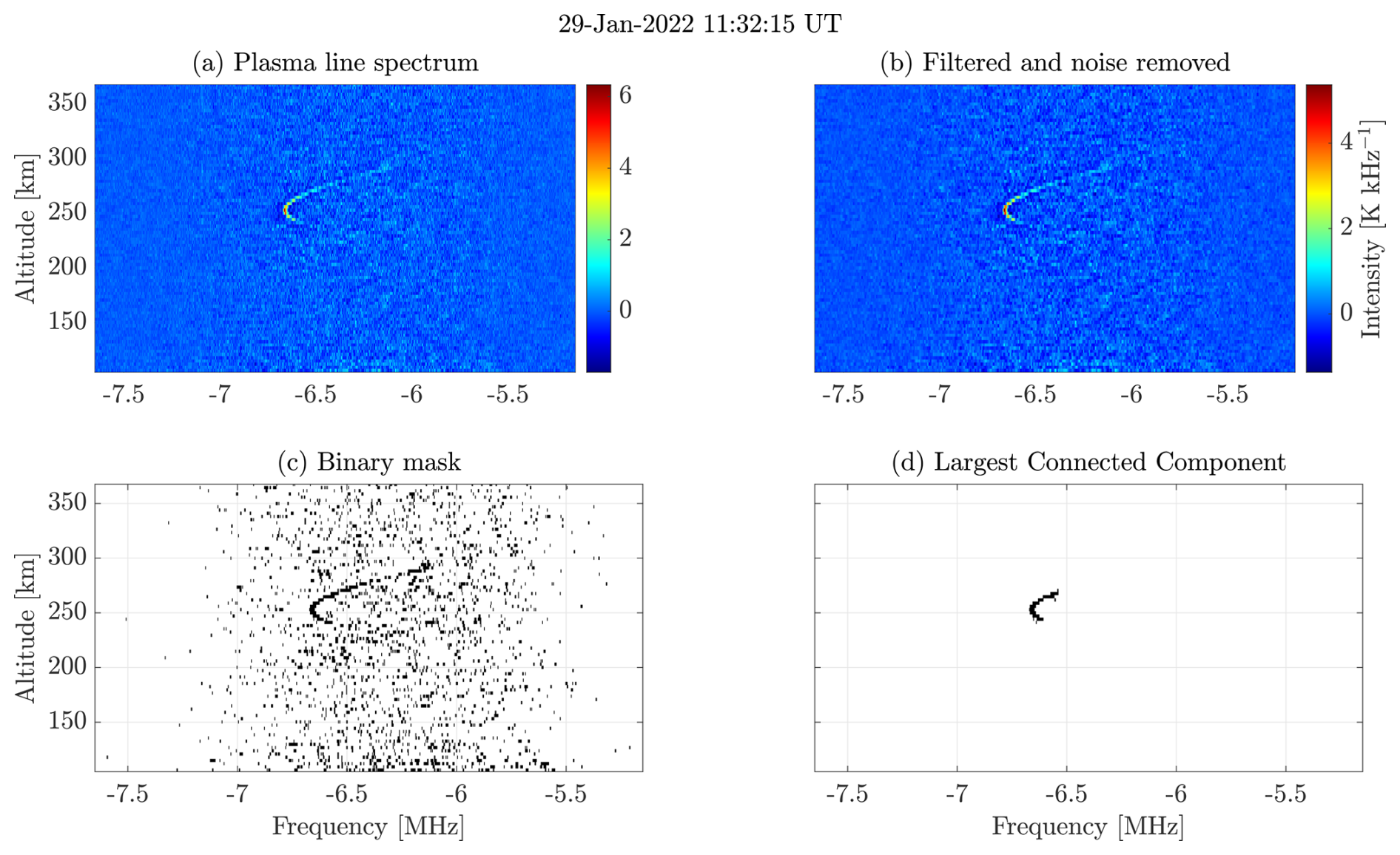
In this analysis, we convert the spectral images into binary images by applying a threshold. A fixed threshold of 2σ_MAD is set to identify pixels with high intensity. After thresholding, each binary image contains multiple connected components, which are groups of adjacent pixels with intensity higher than the threshold. An example is seen in the lower left plot of Fig. 2, where black regions represent distinct connected components. The size of each connected component is given by the number of pixels it comprises. To identify the plasma line signal, we focus on the largest connected component in each binary image, based on the expectation that a significant enhancement in the plasma line signal will result in the largest connected component.

If A_i denotes the number of pixels in the largest connected component of the ith image and there are a total of N spectral images, then the mean, μ, and standard deviation, σ of these largest components across all images are given as:

$$\begin{array}{}\text{(9)}& {\displaystyle }\mathit{\mu }={\displaystyle \frac{\mathrm{1}}{N}}\sum _{i=\mathrm{1}}^N{A}_{\mathrm{i}},\text{(10)}& {\displaystyle }\mathit{\sigma }=\sqrt{{\displaystyle \frac{\mathrm{1}}{N-\mathrm{1}}}\sum _{i=\mathrm{1}}^N|A_{\mathrm{i}}-\mathit{\mu }{|}^{\mathrm{2}}}.\end{array}$$

Let A_min represent the minimum number of connected pixels that the largest component in a binary image must contain to be classified as a plasma line signal. The threshold A_min for detecting plasma lines is set at the three-sigma detection limit, defined as $A_{\text{min}}=\mathit{\mu }+\mathrm{3}\mathit{\sigma }$. The rationale for this threshold is that over a full day of high-frequency spectra recordings, most spectra will contain only random noise. Consequently, the size of the largest connected component in these noisy images will typically be small. Plasma line signals are detectable only during rare specific events such as strong photoionization or auroral precipitation. During these events, the plasma line signal results in a much larger size of the largest connected component. Statistically, this means that events containing plasma lines are outliers. An example is shown in Fig. 3, where a histogram of the largest connected component sizes is plotted for an entire day of spectral recordings. A peak at a size of 30 pixels represents noise-dominated images (Fig. 3). As the size of the largest connected component increases, the histogram decreases, reflecting the rarity of events with the larger size of the largest connected components. The mean size is μ=30, with a standard deviation of σ=21, yielding a threshold of A_min=93 pixels (denoted by the green line in Fig. 3). Any spectral image with the largest connected component of 93 pixels or more is detected as containing an enhanced plasma line, as shown in Fig. 2. Although this threshold A_min may seem high, it effectively avoids false positives in plasma line detection.

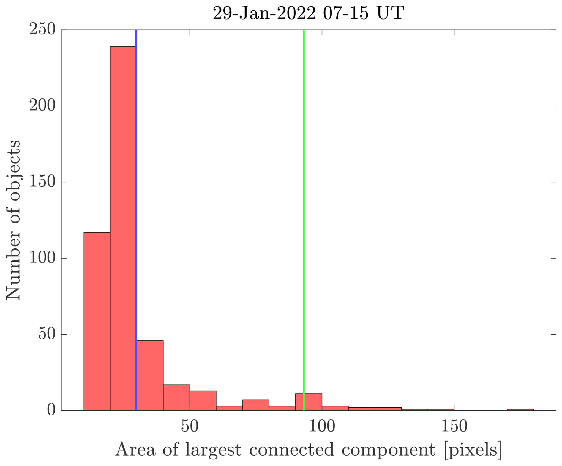
Figure 3 Histogram of pixel counts in the largest connected component from each image on 29 January 2022. The blue line is the mean, μ=30, while the green line is the threshold, $A_{\text{min}}=\mathit{\mu }+\mathrm{3}\mathit{\sigma }=\mathrm{93}$, on the size of the largest connected component for plasma line detection.

A_min is calculated separately for each day and each channel. It is determined automatically from the data as described above rather than manually tuned, ensuring the methodology remains unsupervised. The identification of plasma lines is based only on the statistical outlier of the size of the largest connected components, which makes this methodology data-driven, and hence, unsupervised. This approach is necessary because the noise levels can vary between channels, and calculating a single threshold across all channels could skew the result due to these differences in noise distribution.

3.3 Plasma line parameter extraction

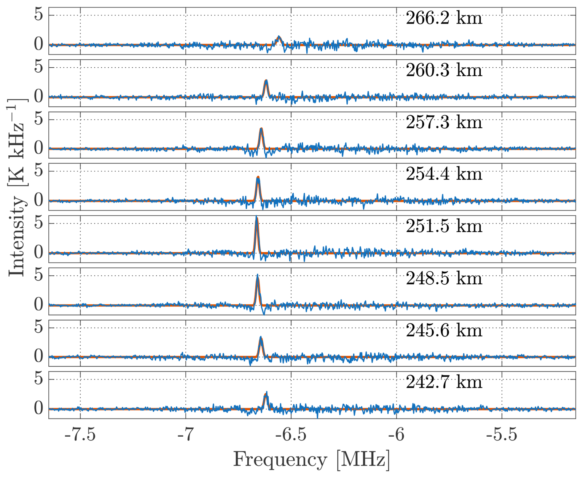
At this stage, we have identified the detection times of the plasma lines. The altitudes where plasma line enhancement occurs are indicated by the final mask in the bottom-right plots of Figs. 1 and 2. At these altitudes, the plasma line is modelled using a Gaussian function characterized by three parameters: intensity A_p, frequency f_r, and half-bandwidth δ_f. To extract these parameters, we used a non-linear, unweighted least-squares Levenberg–Marquardt algorithm, similar to the approach proposed by Guio et al. (1996). As shown in Fig. 4, the spectra were fitted to a Gaussian function

$$\begin{array}{}\text{(11)}& S(f;A_{\mathrm{p}},f_{\mathrm{r}},{\mathit{\delta }}_{\mathrm{f}})={\displaystyle \frac{A_{\mathrm{p}}}{\sqrt{\mathrm{2}\mathit{\pi }}{\mathit{\delta }}_{\mathrm{f}}}}\exp \left(-{\displaystyle \frac{(f-f_{\mathrm{r}}{)}^{\mathrm{2}}}{\mathrm{2}{\mathit{\delta }}_{\mathrm{f}}^{\mathrm{2}}}}\right).\end{array}$$

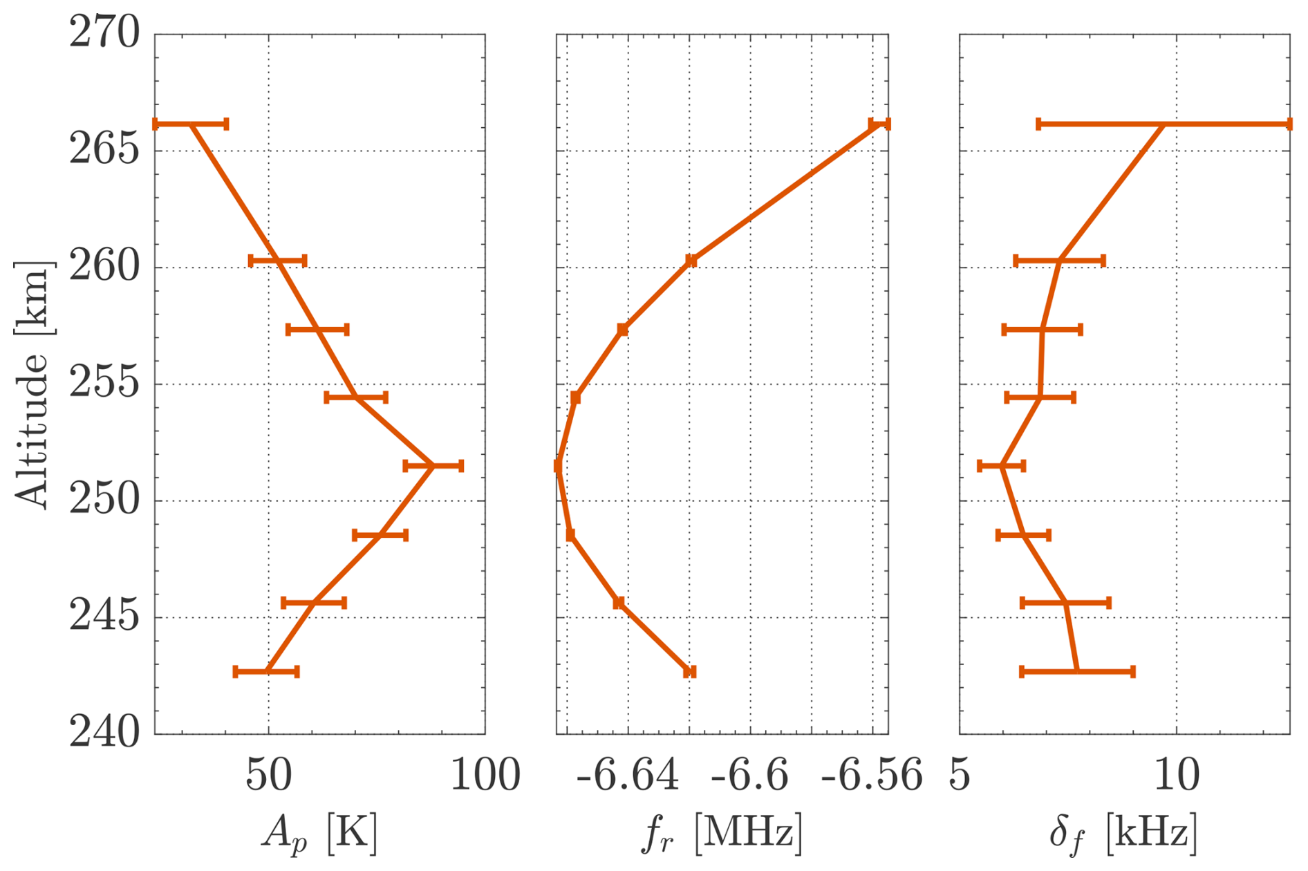
Figure 5 shows altitude profiles of the extracted parameters from Fig. 4 and their uncertainties. The uncertainties were estimated for a 95 % confidence intervals around the parameter estimates.

Figure 4 Plasma line spectra from Fig. 1a (top left plot) at altitudes selected by reduced mask in Fig. 1f (bottom right plot). The blue lines are ISR spectra at selected altitudes, while the red lines are Gaussian model fit.

Figure 5 Altitude profiles of the plasma line parameters (intensity A_p, frequency f_r and half-bandwidth δ_f) from the fit in Fig. 4. Error bars show 95 % confidence level in the fitted parameters. The intensity A_p represents the plasma line antenna temperature ($T_{\mathrm{A}}^{\mathrm{p}}$).

3.4 Derivation of plasma line temperature

A more meaningful form of expressing plasma line intensity is in terms of plasma line temperature (Yngvesson and Perkins, 1968; Fredriksen et al., 1992; Guio et al., 1996; Nilsson et al., 1996) because it allows comparing the plasma line intensity with the theoretical prediction (Fredriksen et al., 1992; Guio et al., 1998) and helps understand how much the plasma line is enhanced above the thermal level. Simultaneous ion and plasma line measurements can be utilized to derive the plasma line temperature (Yngvesson and Perkins, 1968; Fredriksen et al., 1992). In the case of a monostatic radar, the total received power in the plasma line can be expressed by the following radar equation (Yngvesson and Perkins, 1968)

$$\begin{array}{}\text{(12)}& k_{\mathrm{B}}{T}_{\mathrm{A}}^{\mathrm{p}}{B}_{\mathrm{W}}={\displaystyle \frac{P_{\mathrm{T}}}{R^{\mathrm{2}}}}{r}_{\mathrm{e}}^{\mathrm{2}}{\mathit{\sigma }}_P{\displaystyle \frac{c\mathit{\tau }}{\mathrm{2}}}A\left(\mathit{\nu }\right),\end{array}$$

where $T_{\mathrm{A}}^{\mathrm{p}}$ is the antenna temperature of the plasma line, B_W is the bandwidth of the plasma line channel, P_T is the transmitted power, R is the distance between the radar and the volume contributing to the plasma line intensity, r_e is the classical electron radius, $\frac{c\mathit{\tau }}{\mathrm{2}}$ is the length of the range-gate that contributes to the plasma line signal (assuming uniform power distribution over the volume), and A(ν) is the effective antenna area at frequency ν. σ_P is the scattering cross-section contributing to the plasma line, given by Yngvesson and Perkins (1968) and Guio (1998)

$$\begin{array}{}\text{(13)}& {\mathit{\sigma }}_{\mathrm{P}}={\displaystyle \frac{T_{\mathrm{p}}}{T_{\mathrm{e}}}}{\displaystyle \frac{\mathrm{1}}{\mathrm{2}}}{n}_{\mathrm{e}}{k}_{\mathrm{s}}^{\mathrm{2}}{\mathit{\lambda }}_{\mathrm{D}}^{\mathrm{2}},\end{array}$$

where T_p is the plasma line temperature, and k_s is the scattering wavenumber. For the plasma line, k_s differs from that of the ion line because it depends on the centre frequency f_offset of the plasma line wideband receiver. For a radar operating at frequency f_radar and a plasma line receiver centred at f_radar+f_offset, the receiving wavenumber k_r is

$$\begin{array}{}\text{(14)}& k_{\mathrm{r}}={\displaystyle \frac{\mathrm{2}\mathit{\pi }(f_{\text{radar}}+f_{\text{offset}})}{c}}.\end{array}$$

Therefore, for backscattering, the scattering wavenumber is

$$\begin{array}{}\text{(15)}& k_{\mathrm{s}}={\displaystyle \frac{\mathrm{2}\mathit{\pi }(\mathrm{2}{f}_{\text{radar}}+f_{\text{offset}})}{c}}.\end{array}$$

As seen in Eq. (13), the plasma line temperature depends on the scattering wavenumber. This means that ISRs operating at different frequencies have different sensitivities to plasma lines and probe different energy regions within the suprathermal electron velocity distribution. The resonance condition is satisfied when the velocity of the electrons matches the phase velocity of the radar scattering wave. The plasma line frequency shift f_r satisfies the relation along the scattering direction

$$\begin{array}{}\text{(16)}& \mathrm{2}\mathit{\pi }{f}_{\mathrm{r}}=k_{\mathrm{s}}{v}_{\mathit{\varphi }},\end{array}$$

where v_ϕ is the phase velocity of the received wave. This phase velocity is given by:

$$\begin{array}{}\text{(17)}& v_{\mathit{\varphi }}={\displaystyle \frac{f_{\mathrm{r}}c}{\mathrm{2}{f}_{\text{radar}}+f_{\text{offset}}}}.\end{array}$$

Therefore, the corresponding matching kinetic energy of the electrons is

$$\begin{array}{}\text{(18)}& E_{\mathit{\varphi }}={\displaystyle \frac{\mathrm{1}}{\mathrm{2}}}{m}_{\mathrm{e}}{v}_{\mathit{\varphi }}^{\mathrm{2}}={\displaystyle \frac{\mathrm{1}}{\mathrm{2}}}{\displaystyle \frac{m_{\mathrm{e}}{f}_{\mathrm{r}}^{\mathrm{2}}{c}^{\mathrm{2}}}{(\mathrm{2}{f}_{\text{radar}}+f_{\text{offset}}{)}^{\mathrm{2}}}}.\end{array}$$

Since in our experiment, the radar operating frequency, f_radar=931 MHz and the plasma line receiver offset frequency, f_offset, is only a few MHz (less than 1 % of f_radar), the phase energy can be approximated as:

$$\begin{array}{}\text{(19)}& E_{\mathit{\varphi }}\simeq {\displaystyle \frac{m_{\mathrm{e}}{f}_{\mathrm{r}}^{\mathrm{2}}{c}^{\mathrm{2}}}{\mathrm{8}{f}_{\text{radar}}^{\mathrm{2}}}}.\end{array}$$

Thus, an ISR operating at a lower frequency (e.g., EISCAT VHF at 224 MHz) is more sensitive to electrons with larger velocities in the tail of the suprathermal velocity distribution. As a result, such radars can detect subtle features in the high-energy tail of the distribution like peaks at 24.25 and 26.25 eV caused by the ionization of N₂ and O from solar HeII radiation (Guio and Lilensten, 1999) or auroral beams. Conversely, an ISR operating at a higher frequency (e.g., EISCAT UHF at 931 MHz) is more sensitive to electrons with lower velocities. Thus, a higher-frequency ISR might be better suited for studying features like the 2–4 eV N₂ dip (Fredriksen et al., 1992; Kirkwood et al., 1995; Nilsson et al., 1996). Using multiple ISRs at different frequencies gives the ability to probe different velocity ranges, making it possible to construct a picture of the plasma line spectra due to different features in the suprathermal velocity distribution.

4 Results

The analysis of plasma line data using the supervised methodology revealed detectable enhancements for about 10 % of the total observational time. Plasma lines were observed 26 %, 5 % and 5 % of the total pointing time in the field-aligned, east and vertical directions, respectively. Over the entire analysis period (26–31 January 2022 with 8 h per day between 07:00–15:00 UT, except on 26 January between 08:00–15:00 UT), the unsupervised methodology detected 110 plasma lines, while the supervised methodology detected 275. Both methodologies are robust against noise factors such as (a) localized noise at specific altitudes, as shown in Fig. 6, and (b) higher noise around the centre frequency of the filters where the plasma line profile is superimposed, as shown in Fig. 7. The filtering and noise removal technique from Ivchenko et al. (2017) enhances plasma lines despite these challenges, facilitating plasma line profile detection. Here, we present the results of the analysis for 29 January 2022 07:00–15:00 UT only.

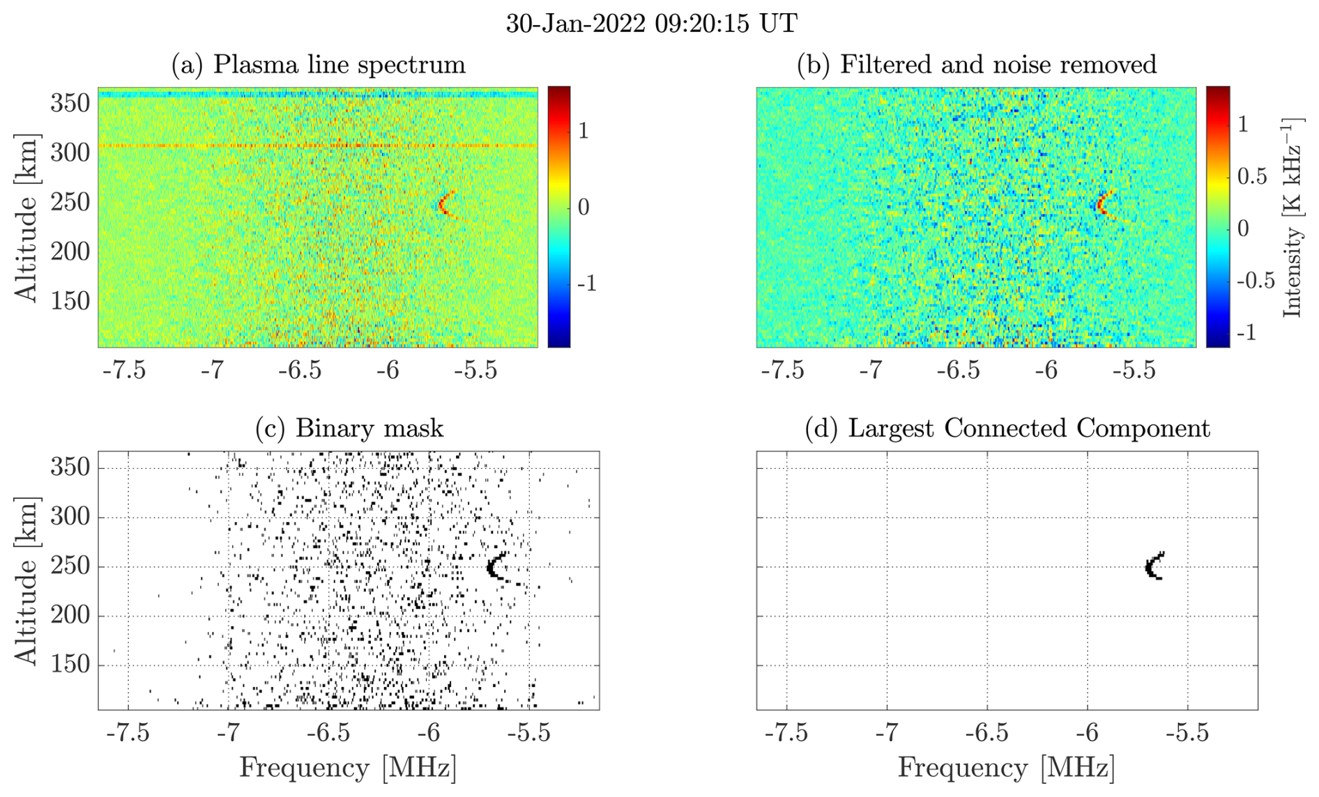
Figure 6 (a) Plasma line spectrum observed by EISCAT UHF radar, showing strong wideband noise localized at 307 and 360 km. (b) Filtering and noise removal eliminate the localized noise. (c) and (d) show the plasma line detection using the unsupervised methodology illustrated in Fig. 2.

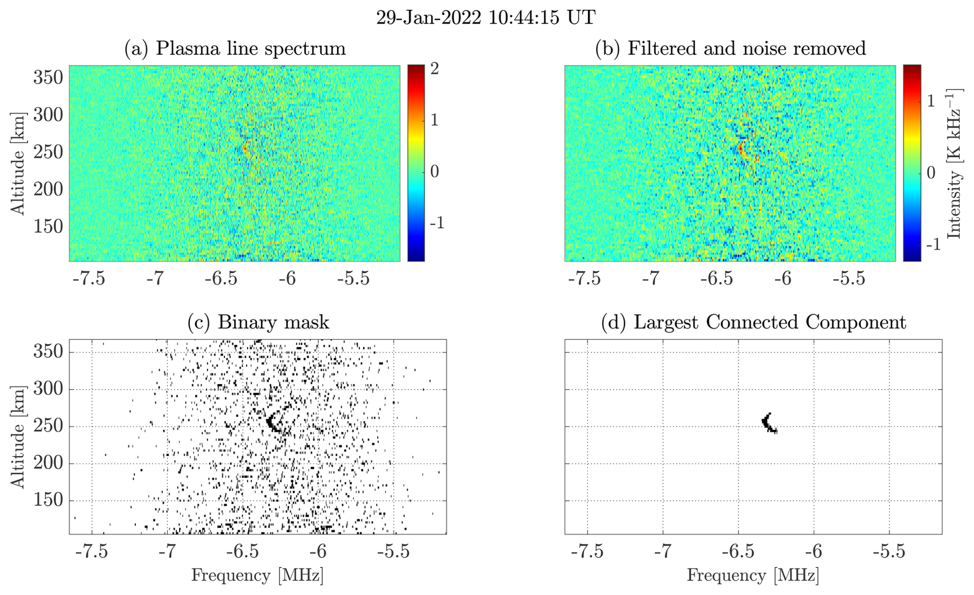
Figure 7 (a) Same as Fig. 6, but showing the case where the plasma line profile is superimposed on the high noise around the centre frequency from −7 to −6 MHz. (b) The filtering and noise removal method effectively enhances the plasma line while suppressing the noise. (c) and (d) show the plasma line detection using the unsupervised methodology illustrated in Fig. 2.

The plasma line data fit well to the Gaussian model (see Fig. 4), as was also shown in Guio et al. (1996). Figure 5 shows the altitude profile of the plasma line parameters derived from the fit in Fig. 4. It can be seen that the derived plasma line frequency exhibits a smooth variation in altitude, with the maximum in the magnitude of plasma line frequency at the F2 peak altitude of 251.5 km. This behaviour is due to the plasma frequency's quasi-parabolic variation with altitude around the peak at hmF2, as pointed out in Guio et al. (1996). Near the F-layer peak, the reduced frequency spreading leads to a stronger and narrower plasma line at the altitude with the highest electron density. In contrast, the steeper gradient of the plasma frequency away from the peak causes more frequency spreading of the plasma line signals above or below the F-layer peak. This trend is evident in Figs. 4 and 5, where the plasma line width is narrowest at the F2 peak and gradually broadens above and below this altitude.

Figure 8 shows the electron density and temperature estimates as a function of time and altitude obtained from GUISDAP using the ion line data from 29 January 2022. A scaling parameter known as the Magic constant must be specified in GUISDAP for the ion line analysis. The Magic constant is calibrated to ensure that the electron density derived from the plasma line matches that obtained from the ion line. A different Magic constant was calculated for each day of the experiment. GUISDAP assumes Maxwellian electron and ion velocity distributions to estimate these parameters. The parameters are plotted over the same time period, from 07:00 to 15:00 UT, and the same altitude range, 107–374 km (see Table 2), where the plasma lines were analyzed. The black vertical lines indicate the time interval during which plasma lines were detected using the supervised methodology as demonstrated in Fig. 1. During this interval, electron density increases to $\approx \mathrm{5}\times {\mathrm{10}}^{\mathrm{11}}{\mathrm{m}}^{-\mathrm{3}}$, corresponding to a plasma frequency of ≈ 6 MHz, between 230 and 280 km, i.e. around the F-layer peak where scale height is largest. As a result, most of the plasma lines observed are in the same altitude range. Figure 9 shows the estimated plasma line parameters as function of time and altitude derived using the plasma line parameter extraction technique (see example provided in Figs. 4 and 5) from all positive plasma line detections at different times and altitudes on 29 January 2022, following the supervised methodology illustrated in Fig. 1, with analysis similar to Guio et al. (1996).

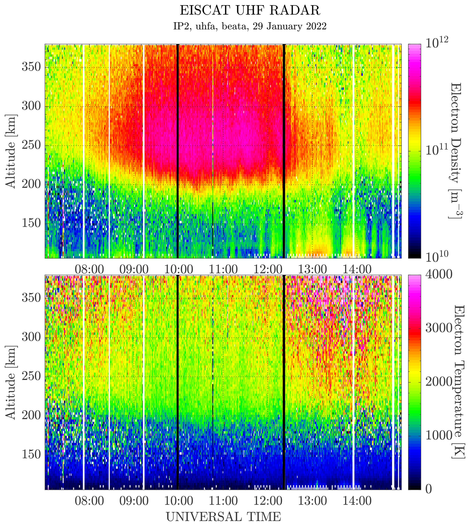
Figure 8 Electron density and temperature estimated from ion line analysis using GUISDAP. Black vertical lines indicate the period of plasma line detection by the supervised methodology, with electron density enhancements from photoionization observed between these lines.

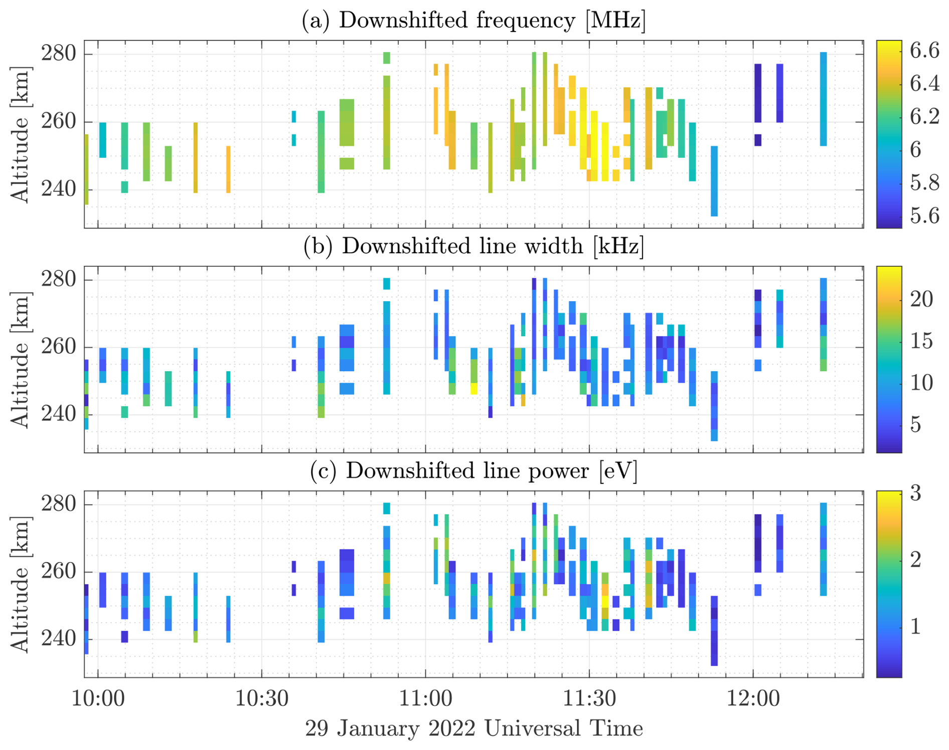
Figure 9 Estimated parameters of the downshifted plasma line as a function of altitude and time on 29 January 2022, using the methodology illustrated in Fig. 4 during the period marked by black vertical lines as shown in Fig. 8. (a) Doppler frequency (f_r); (b) half-bandwidth (δ_f); (c) intensity (k_BT_p). Colour bars indicate parameter magnitudes.

The plasma line is observed only in the downshifted channel, with frequency magnitudes between 5.5 to 6.7 MHz. The plasma line frequency increases gradually from 10:00–11:20 UT (Fig. 9), driven by an increase in the photoelectron population from solar EUV radiation. An additional feature visible in Fig. 9 is the quasiperiodic undulation of the detected plasma line location, corresponding to vertical shifts of the F-region lower boundary. Similar variations can be seen in the electron density derived from the ion line data (Fig. 8) and were also observed on other days of the experiment. The exact cause of these undulations is uncertain. However, possible drivers such as atmospheric gravity waves or magnetospheric Pc5 ULF waves could be worth investigating in future studies. The plasma line enhancement mechanism itself depends primarily on the presence of suprathermal electrons, and is not directly altered by altitude variations of the F-region boundary.

We have similar plots to those shown in Figs. 8 and 9 for the other days, which are provided in the Supplementary Material (Figs. S1–12). The background electron density and temperatures, as shown in Fig. 8, do not vary significantly from day to day. The variation in background electron density over different days is between $\approx \mathrm{2}\times {\mathrm{10}}^{\mathrm{11}}$ to $\mathrm{9}\times {\mathrm{10}}^{\mathrm{11}}{\mathrm{m}}^{-\mathrm{3}}$. As can be seen from Eq. (19), the phase energy depends on the plasma line frequency and therefore the background electron density. Since the electron density naturally fluctuates from one day to another, the range of the phase energy explored will consequently vary.

5 Summary and discussion

We discussed two methodologies for detecting plasma lines. The first, a supervised approach based on image morphological processing, requires manual tuning of binary threshold and erosion/dilation parameters. This approach requires an initial guess of the parameters followed by iterative adjustments. In our case, we began with the parameters used by Ivchenko et al. (2017) for ESR IPY experiments and refined them until no false positives were detected for a given day and channel. However, selecting parameters in this supervised approach relies heavily on trial and error, requiring many adjustments based on the observation day, radar channel, and radar type. In contrast, the methodology based on connected component analysis is an unsupervised approach, as the detection thresholds are not manually defined but are automatically derived from statistical estimators and the distribution of the connected component sizes. This data-driven approach establishes thresholds for converting spectral images to binary format and for detecting plasma lines in entire datasets for a given day, channel, and radar, eliminating the need for initial assumptions or manual adjustments. As a result, the unsupervised approach is more adaptable to different radars.

The supervised methodology detected more plasma lines than the unsupervised. Both supervised and unsupervised methodologies were tuned to avoid false positives. The supervised methodology may have a higher sensitivity to weaker plasma lines, while the unsupervised with statistically derived thresholds, is more conservative and may miss some weaker signals. Each methodology has its strengths depending on the goals of the analysis. The supervised methodology may be preferable when the goal is to maximize detection sensitivity, while the unsupervised methodology is more suitable for working with large datasets spanning multiple days or different radars.

88 % of the plasma lines detected in the downshifted channels occurred at the magnitude of frequencies above 5.25 MHz, with the lowest detected plasma line frequency across all six days being 4.7 MHz. This means that the plasma lines detected in the downshifted channel between 2.75 to 5.25 MHz occurred near the edge of the filter. In the experiment, no data were recorded in the upshifted channel at frequencies above 5.25 MHz. Although data were recorded at upshifted frequencies between 2.75 to 5.25 MHz, no plasma lines were detected in this range, possibly because plasma lines in downshifted channels likely occur above 5.25 MHz. One of the initial objectives of this study was to estimate ionospheric currents using plasma lines observed at both upshifted and downshifted frequencies. However, the absence of corresponding upshifted plasma lines prevents us from calculating ionospheric currents in the present analysis.

We can nevertheless analyze plasma line intensity as a function of phase energy. This provides fine-grained details about the suprathermal electron velocity distribution at the corresponding velocity range. The phase energy of the plasma line corresponds to the kinetic energy of the electrons that are in resonance with the electrostatic wave. Since the F10.7 index, the electron density and temperature do not exhibit substantial variations across the entire analysis period, we combine data from each day (26 to 31 January 2022 07:00–15:00 UT) to plot the plasma line intensity, k_BT_p, as a function of phase energy, E_ϕ, calculated from the derived plasma line frequency using Eq. (19)

Figure 10 shows plasma line intensity versus phase energy at different altitudes, using plasma line measurements from 26 to 31 January 2022. Plasma line intensity is a function of time, altitude, phase energy and aspect angle; here, we integrate it over time and aspect angles to display it as a function of phase energy and altitude. The figure uses box plots to represent plasma line intensity across uniform phase energy intervals: each box's central line shows the median plasma line intensity, with top and bottom edges indicating the upper and lower quartiles (the 75th and 25th percentiles, respectively). The interquartile range (IQR) is the distance between these quartiles. Outliers, defined as samples exceeding 1.5⋅IQR from the top or bottom of the box, are represented by the symbol “o”. Additionally, the whiskers extend from each box: one connects the upper quartile to the non-outlier maximum (the highest value that is not an outlier), and the other connects the lower quartile to the non-outlier minimum (the lowest value that is not an outlier).

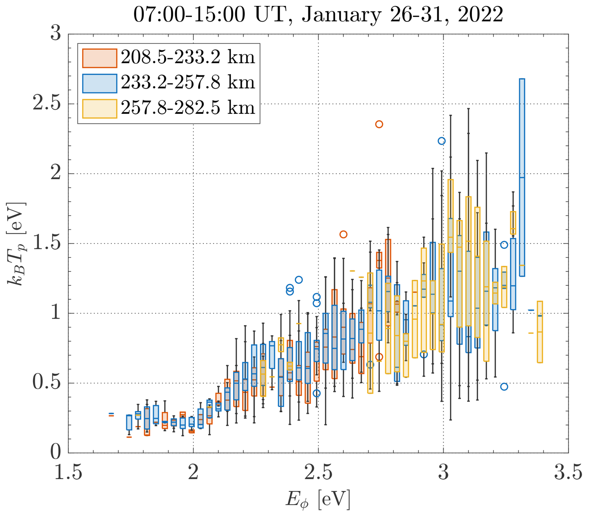
Figure 10 Plasma line temperature k_BT_p as a function of phase energy E_ϕ, integrated over time and aspect angles, and binned by altitude.

As seen in Fig. 10, plasma line intensities are grouped into three altitude ranges. 66 % of the plasma lines are detected between 233.1–257.8 km (corresponding to the range around the F2 peak), 22 % detected between 208.5–233.2 km (below the F2 peak) and 12 % detected between 257.8–282.5 km (above the F2 peak). The highest-frequency plasma line observed occurred at 6.76 MHz, corresponding to an altitude of about 246 km, which lies near the middle of the altitude range where plasma lines were detected. As can be seen in Fig. 4, the intensity of the plasma line is largest around the F2 density peak, which explains why most of the plasma lines are observed in the range 233.1–257.8 km.

The plasma line frequency bands extend from −7.65 to −2.75 MHz, as described in Sect. 2. Using Eq. (19), it can be determined that the EISCAT UHF system can probe an energy interval of 0.6–4.4 eV. However, as shown in Fig. 10, the observed plasma lines are confined to the energy range of 1.7–3.4 eV. This indicates that, despite detecting hundreds of plasma lines, only 45 % of the total phase energy range accessible is effectively explored. This suggests that, even with multiple days of observations, the daytime ionospheric conditions between consecutive days were relatively similar. While plasma lines with phase energies below 1.7 eV may exist, they are likely obscured by noise due to the lower plasma densities, and therefore, lower SNR.

As the resonance phase energy increases, the plasma line intensity increases for all the altitude groups, peaking around a phase energy of 3 eV, after which it starts decreasing again. This result is consistent with the model predictions by Nilsson et al. (1996) where F-region photoelectron-enhanced plasma lines observed by EISCAT UHF radar peaks at approximately 2.7 eV. The variation in plasma line intensity can be understood in terms of the balance of several damping and excitation mechanisms, including collisional damping, thermal Landau damping, and photoelectron Landau damping (Akbari et al., 2017; Longley et al., 2021). For phase energies below 4 eV, the dominant processes are thermal Landau damping and Cerenkov excitation of thermal electrons (Nilsson et al., 1996; Akbari et al., 2017). The magnitude of Landau damping depends on the slope of the reduced one-dimensional velocity distribution function of the electrons along the direction of the scattering wave vector. Smaller Landau damping corresponds to larger plasma line intensity. The presence of a suprathermal electron population introduces a high-energy tail to the distribution function, decreasing the slope at higher energies and thereby, reducing Landau damping. Consequently, as phase energy increases, the plasma line intensity increases. This differs from higher phase energies, where inverse Landau damping of photoelectron peaks can provide an additional source of wave growth (Longley et al., 2021). It is also worth noting there do not seem to be any significant or systematic differences in plasma line intensity between the altitude groups for any given energy, indicating that the suprathermal populations are very similar at these altitudes.

Figure 11 presents plasma line intensity as a function of phase energy for the available aspect angles and integrated over altitude and the six days from 26–31 January 2022 07:00–15:00 UT. The data are visualized as box plots similarly to Fig. 10. It can be seen that the plasma line intensity generally decreases as the aspect angle increases. This result is consistent with the findings of Yngvesson and Perkins (1968); Fredriksen et al. (1992) that accounted for the magnetisation of suprathermal electrons in their derivation. Yngvesson and Perkins (1968) suggested that the Landau damping increases with the aspect angle. This implies that the reduced one-dimensional electron velocity distribution function becomes steeper at higher aspect angles, meaning that more electrons absorb energy from the wave. This can be a possible reason for the reduction in plasma line intensity at higher aspect angles. More recent work by Longley et al. (2021) shows that plasma line intensity is roughly constant up to ∼ 10° and increases between 10–20°. In their study, the intensity variation in the phase energy regime is dominated by the inverse Landau damping of the photoelectron peaks. For the relatively low phase energies considered here (< 4 eV), however, the dominant mechanisms governing the observed variations remain Landau damping and Cerenkov excitation (Nilsson et al., 1996; Akbari et al., 2017), and a detailed modelling with suprathermal electron distribution is left for future work.

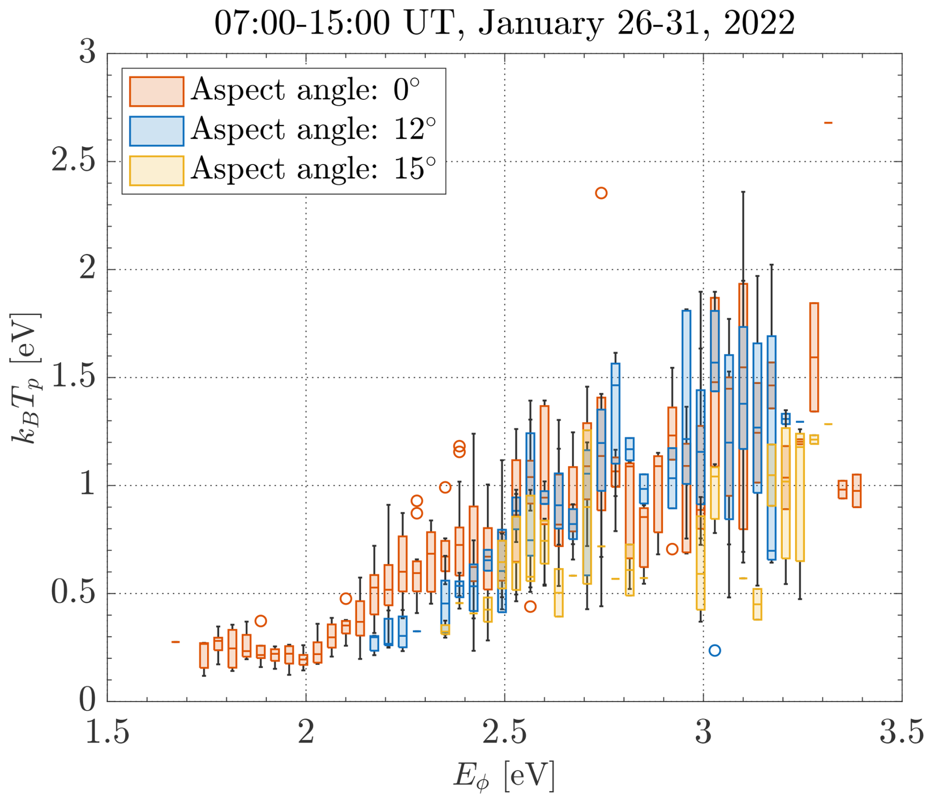
Figure 11 Plasma line temperature k_BT_p as a function of phase energy E_ϕ, integrated over time and altitude, and binned by aspect angle.

Even though the data are taken from multiple days covering different phase energy intervals, there is an overall smooth variation of plasma line intensity with phase energy as seen in Figs. 10 and 11. This suggests that the suprathermal electron velocity distribution at the corresponding velocities does not vary significantly over the observation campaign.

Plasma line enhancements above the thermal level depend directly on the suprathermal electron flux. During daytime, the prolonged input of solar EUV energy produces suprathermal electron fluxes over an extended period, resulting in more frequent plasma line detections, particularly around the F-layer peak where electron density is highest. At night, suprathermal electron flux is generated through transient auroral activity, resulting in observable plasma line enhancements. For nighttime observations, careful selection of the integration time is necessary, as too long an interval could average out short-lived enhancements and make plasma lines harder to detect.

Regarding seasonal variations, we expect statistical plasma line occurrence to vary in line with the study from Ivchenko et al. (2017). In particular, May–July will offer the highest number of plasma line observations due to prolonged solar illumination and high suprathermal electron fluxes. Both solar EUV radiation and auroral precipitation can contribute during March–April and August–October, allowing plasma line detection under a wider range of conditions. Therefore, there can be more observations over wider phase energy intervals to build figures similar to Figs. 10 and 11 for plasma lines observed due to both solar EUV radiation and auroral precipitation.

The primary objective of the present paper is to develop a processing pipeline and demonstrate that methodology for plasma line detection and analysis. The methodology presented can be applied in future long-term studies to investigate how plasma line occurrence and phase energy distributions vary with season, time of day, and aspect angle. A proper exploration of the seasonal and diurnal variations would require multiple observations spanning the year under varying conditions, which is beyond the scope of the current work but could be pursued in future studies.

Previous studies (Nilsson et al., 1996; Guio et al., 1998; Guio and Lilensten, 1999) have modelled plasma line intensity using suprathermal electron population angular differential energy fluxes computed by an ionospheric electron transport code (Lummerzheim and Lilensten, 1994). Building on the plasma line model described in Guio et al. (1998), we aim to further develop an aspect angle dependent plasma line intensity model and apply it to the current dataset. This approach, which will be detailed in a future paper, will use the general-purpose plasma line analysis pipeline we developed here. Unlike previous models (Longley et al., 2021), which assumed isotropic electron distributions and did not include pitch-angle dependence, our approach will build on the framework of Guio et al. (1998); Guio and Lilensten (1999) and incorporates numerical electron transport modelling to obtain anisotropic electron velocity distribution functions. This will allow for a more realistic treatment of photoelectron populations under local geomagnetic conditions in incoherent scatter spectral modelling.

The methodologies presented here have facilitated the detection of hundreds of plasma line events, significantly increasing the volume of data available for theoretical validation compared to previous studies. The only limitation of the dataset is the number of pointing directions to the magnetic field which is imposed by the experiment design. This is where advanced radar systems like EISCAT 3D (McCrea et al., 2015) will be useful. Unlike the current EISCAT systems with mechanically steered antennas, EISCAT 3D with phased array antenna technology will enable the beam to be steered at different aspect angles with higher time resolution. This capability will greatly expand the dataset for studying the aspect angle dependence of plasma line parameters.