High-latitude auroral and cloudiness occurrence from automatic image classification

We have investigated auroral and cloudiness occurrence over Kjell Henriksen Observatory (KHO) in Svalbard using full-colour all-sky images from 2016–2025. Our approach focused on constructing a high-quality manually labelled training set, in which images were classified as ClearAurora, ClearNoAurora, CloudyAurora, or CloudyNoAurora based on their content. As there is an inherent overlap between these classes, we carried out several iterative validation rounds to increase the number of high-quality sample images and to remove images with unclear contents in the training set. We then evaluated different Convolutional Neural Network topologies and selected the best performing network to classify all images between January 2016 and December 2025 (over 8 million images in total). In addition to the validation accuracy with the ground truth, we also estimated the classification accuracy based on a random selection of classified images. Our final classifier, called KHOnet2026, results in accuracies from 94 % to 98 % depending on the image class.

We found that most of our image data is cloudy (60 %–70 %). A validation of the cloud occurrence results was performed with an independent dataset from a co-located cloud sensor. We found a good agreement between the two datasets at a monthly average level with a correlation coefficient of 0.86. Auroral occurrence over Svalbard is of the order of 25 % of the imaging time, and it shows no solar cycle correlation but is rather modulated by the cloudiness. The portion of clear skies without aurora is only about 10 %. Statistically, the clearest month at KHO is January and the cloudiest one is November. This automatic classification routine is set to run in real-time and further expand the database of classified images to aid researchers in finding images with aurora. Excluding the cloudy data allows a far more efficient use of computer time in more detailed analysis of, for instance, the structural evolution of the aurora. Furthermore, the automatically classified images provide a helpful proxy for all other optical instruments hosted by KHO.

1 Introduction

Auroral imaging has been a standard observation technique in near-Earth space environment studies since the 1970s and 1980s. However, long-term analyses of auroral occurrence based on these data have mainly been performed manually. For instance, Nevanlinna and Pulkkinen (2001) used a time series of the types of aurora over 25 years from 7 different camera locations spanning about 15° in latitude across the auroral oval. Aurora types were visually determined from all-sky films in 15 min video snippets. They concluded that there is no obvious correlation between auroral occurrence (AO) and the solar cycle evolution. Instead, an increasing trend was detected in 1973–1993, which was interpreted as a signature of a long-term increase in the solar activity. As discussed by the authors, a longer-term correlation between aurora and solar activity has been reported at mid-latitudes and appears at the auroral oval latitudes as an occurrence of different types of aurora during the active and quiet conditions. While quiet auroral structures dominate the years of solar minimum, the occurrence of active aurora increases during the solar maximum (Nevanlinna and Pulkkinen, 1998). A similar variation in the complexity of the auroral structures was later reported as a result of an automated analysis of auroral structures on already pruned image data from the auroral oval latitudes (Partamies et al., 2014), while the auroral occurrence evolution over a solar cycle time scale has not been systematically investigated beyond the studies by Nevanlinna and Pulkkinen (2001) and Pulkkinen et al. (2011).

For most auroral image analysis tasks a straightforward approach is supervised learning, where examples of data with class labels are provided as the “ground truth” or the correct answers. The ground truth is used to train a classifier, which then provides a label to previously unseen images. Intuitively, having more examples of various data improves the results. However, this also means that we need a very large set of labelled data to achieve good results. For example, Rao et al. (2014) categorised 33 000 auroral images into classes of Aurora, NoAurora and Cloudy. They used a Support Vector Machine (SVM) classifier coupled with an Opponent Scale Invariant Feature Transform (SIFT) feature extraction method, which resulted in an accuracy of 91 % in validation and 80 % in test. The classification result was further improved by post-processing steps to remove twilight images and ignore class changes for individual images in a time series.

More recent studies have performed auroral image classification with a larger number of classes, typically including arcs, patchy/diffuse, discrete, moon, clear and clouds (e.g. Clausen and Nickisch, 2018; Kvammen et al., 2020; Sado et al., 2022; Nanjo et al., 2022; Hu et al., 2024). These methods also achieve classification results with a success rate of about 90 %. At least half of the data contain no aurora (classes of clear skies, clouds, Moon), whereas the classes containing aurora are very broad. Classifying a combination of aurora and non-aurora images makes the morphological part of the classification inefficient. As Syrjäsuo and Donovan (2004) pointed out, less than 10 % of all auroral forms can be named by auroral researchers, which makes the ground truth difficult to determine. To overcome the problem of classifying largely unknown auroral features, an auroral arciness index was introduced to include all images that contain aurora (Partamies et al., 2014). This method calculates a number between 0.4 and 1 to describe how arc-like the distribution of the brightest pixels in an image is. It has, for instance, been used to characterise structural evolution of poleward moving auroral forms in the dayside aurora (Goertz et al., 2023). However, to produce meaningful results the method requires the input data to contain aurora.

To avoid the massive manual labelling effort required for supervised learning, methods such as semi-supervised or self-supervised learning are being developed (Rani et al., 2023). In the recent study, Johnson et al. (2024) used a contrastive learning objective in analysing THEMIS all-sky images. First, latent representations of image contents were learned in an unsupervised fashion from roughly 910 000 images. In the second stage, the authors constructed a classifier to provide class labels to the latent representations. This was carried out by using supervised learning and (only) roughly 6000 labelled images. The authors demonstrated the power of the methodology by analysing about 700 million THEMIS images taken at the auroral oval latitudes. This gave statistically meaningful results: auroral occurrence centered around magnetic midnight and arcs relating to milder geomagnetic activity than discrete and diffuse aurora.

Currently the only operational machine learning-based classification for auroral all-sky images is by Nanjo et al. (2022). Their dataset for training and method development consisted of full-colour images from one camera station at auroral latitudes (in Tromsø, Northern Norway) captured in 2011–2021. They used supervised learning with ResNet-50 network and 8 classes, largely following the previous work by Kvammen et al. (2020). They also added supplementary classes for, for example, twilight conditions where the bright blue background sky makes auroral emission difficult to detect. With a set of about 90 000 manually labelled images they reported an average classification accuracy of 93 %. Their long-term analysis of auroral occurrence suggests seasonal highs around equinoxes and an annual evolution that closely follows the local geomagnetic activity, i.e. reaching a maximum in the early declining phase of the solar cycle and minimum during the solar cycle minimum.

Another type of operational auroral detection method was developed by Yamauchi and Brändström (2023), based on thresholding and classifying RGB pixel values of the auroral all-sky images. This method is detecting and alerting on local auroral brightenings (https://www.irf.se/alis/allsky/nowcast/, last access: 28 September 2026) over Kiruna in northern Sweden in realtime with an estimated accuracy of 90 %.

In this study, we analyse the typical evolution of auroral and cloudiness occurrence at the latitudes of the poleward boundary and dayside auroral oval by automatically detecting both phenomena with accuracies of the order of 95 %. We have constructed a set of ground-truth images through a number of iterations to develop and evaluate different image classifiers. Our best-scoring classifier, called KHOnet2026, is implemented to run and expand our statistics in realtime, so that investigations of changes in the auroral and cloudiness occurrence can be carried out with minimal effort. Our results can be used as metadata for the sky conditions at the Kjell Henriksen Observatory (KHO), which hosts a large number of instruments used for auroral research (Herlingshaw et al., 2024). By being able to focus on images with relevant content, follow-up studies (similar to e.g. Partamies et al., 2024) can be carried out more efficiently.

Auroral image data are described in Sect. 2. Section 3 summarises the pre-processing and classification of the images, and Sect. 4 contains results from both the methodological perspective and from the long-term auroral evolution. Discussion and Conclusion are presented in Sects. 5 and 6.

2 Auroral image data

We use full-colour all-sky camera (ASC) data from Kjell Henriksen Observatory (KHO) located at 78.25° N, 16.04° E, and at geomagnetic latitude of 75.20° N in Svalbard, arctic Norway. The instrument setup comprises a computer controlling a Sony α7s mirrorless full-frame camera with an all-sky lens. Whenever the Sun is more than 10° below the horizon, images with a 4 s exposure time are captured at a cadence of 12 s throughout the polar night, which in Svalbard extends from the beginning of November until the end of February. During some years, some data have also been collected in March and October, but since those months are very sparsely covered, we limit our analysis to the Northern Hemisphere winter months from November to February. During the first operational months in autumn 2015, different imaging modes were evaluated before the best suited options were selected for routine measurements in early 2016. In this study, we therefore only include the images from the beginning of 2016 onwards. The ASC raw data consist of 8 bit RGB colour images with a high pixel resolution (2832×2832) stored in JPEG-format. However, our analysis uses only quicklook data with a reduced pixel resolution (480×480) for faster processing. All quicklook image data used in this study are available at the AuroraX platform (Donovan et al., 2020).

Sony ASC also has comparable predecessors since 2008, including several Nikon DSLR models with similar all-sky optics. These cameras were in operation from 2008 to 2016. The data are 8 bit RGB images with 2464×2464 pixel resolution with a 30 s cadence. The overlapping imaging with the two camera systems in 2016 has been used to test how well a classifier trained on Sony data performs on Nikon images without any additional training.

3 Classification method

3.1 Methodology

In this study, we use supervised learning to classify auroral images. A human expert is therefore needed to provide examples with correct class labels, or the ground truth. The knowledge of correct labels allows us to use this ground truth to train a classifier to minimise the classification error. Commonly, the classifier itself is a non-linear function such as a neural network and the optimisation is an iterative process governed and guided by a number of hyperparameters. These hyperparameters define, for example, how much the classifier can be adjusted (“trained”) during one epoch. An epoch is one complete pass of training set during which the classifier's internal parameters are modified to improve performance (correct classification). At the end of each epoch, the classification error is estimated and, if the desired accuracy not yet reached, another epoch is run. A recommended practice is to divide the ground truth into training and validation sets, where the former is used in the training and the latter in evaluating the classifier performance during training. Final performance is usually carried out with a completely independent test set, or data not used in training the classifier.

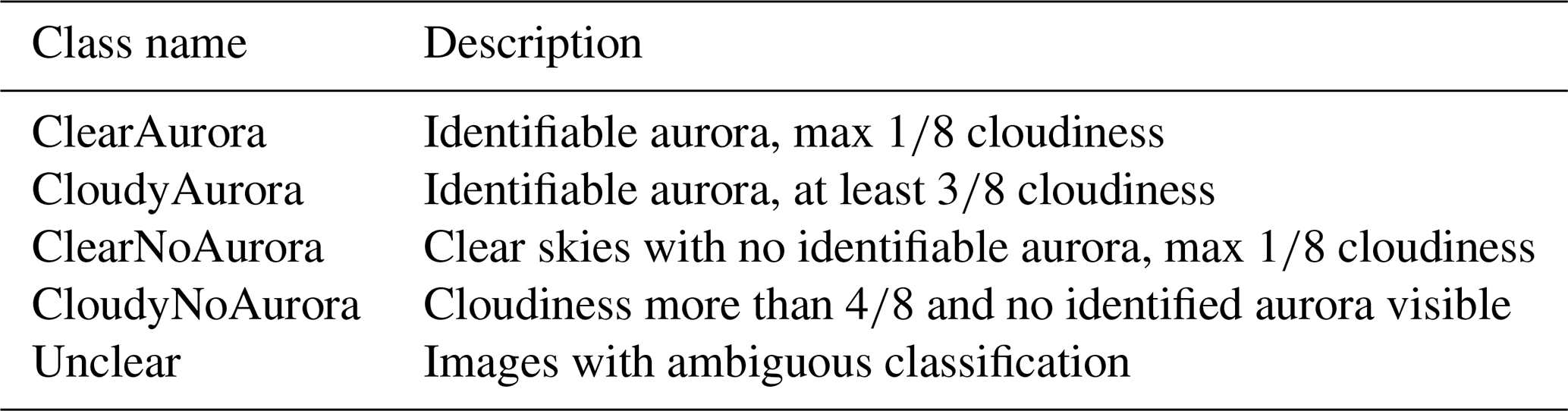
In our case, the input is an auroral image and the output is a vector of probabilities for each class. It should be noted that the output should be interpreted as the probability distribution among the predefined classes rather than actual class probabilities. As our main objective is to separate images with and without aurora, with and without clouds, we use only a few classes that broadly describe the image content. These classes and their definitions are listed in Table 1. A large margin is taken to differentiate between cloudy and clear conditions, because estimating the total cloudiness visually has a large uncertainty to it. We reserve the class “Unclear” for auroral images with ambiguous content, i.e. images without a solid ground truth label. The Unclear class typically consists of images with low but non-zero cloudiness, and/or very faint aurora. A more detailed discussion of the ground truth can be found in Sect. 3.2.

Table 1 Definitions of broad classes used in this study.

In the recent years, Convolutional Neural Networks (CNN, LeCun et al., 2015) have become a popular approach in image classification. A CNN can contain millions of parameters and training such a network requires not only millions of images but also weeks to months of computer time. However, an already trained network can be re-trained with relatively little effort by using transfer learning. In this approach, one chooses an existing pretrained network, makes some changes in the network topology and then trains the network with application specific images such as auroral images. This is the approach used by e.g., Clausen and Nickisch (2018). In a study that evaluated different classification methods using data from our Sony ASC, it was, indeed, concluded that CNN methods with transfer learning performed best with auroral images, but that there was a significant overlap between the different auroral classes (Tachet, 2022). We presume that inaccuracies in these classification results were predominantly due to the quality of the ground truth images rather than poor classifier performance. This became evident when visually inspecting the labelled images.

Guo et al. (2022) utilised several commonly used and openly available CNNs as starting points to compare the classification results of auroral images. In their experiments, all but one CNN reached an accuracy of more than 95 %. This suggests that the choice of CNN used in transfer learning is not particularly critical. In our study, we used GoogLeNet (Szegedy et al., 2016a) as the starting point for transfer learning. GoogLeNet is a relatively small (with “only” 7.0 million parameters), but quite accurate convolutional neural network that has been trained with a massive set of images covering 1000 object categories. It is therefore often used as a starting point for transfer learning in image classification applications. We later evaluated several other network topologies and selected InceptionV3, a much larger CNN with roughly 24 million parameters (Szegedy et al., 2016b), due to its evenly good performance on all classes.

For the transfer learning, we replaced the final classification layers in each CNN to produce an output vector for the probabilities in the four classes of ClearAurora, ClearNoAurora, CloudyAurora, and CloudyNoAurora. The images were randomly divided into training (60 %), validation (20 %) and test sets (20 %) for GoogleNet, while InceptionV3 was run on a division of 70 % for training and 30 % for validation with a dedicated independent test set. The training and validation sets were used in training the CNN and the test set was used in evaluating the final classification accuracy. The auroral images were rescaled to match the input layer in the network; the pretrained networks require input images in different sizes, 224×224 for GoogLeNet and 299×299 for InceptionV3. We also augmented the training set with random horizontal and/or vertical flips as well as up to ±10° rotations of input images. This is a common practice in CNN training to avoid overfitting and to improve convergence. The source code with more details about the modifications is available at https://github.com/UNISvalbard/KHOnet2026 (last access: 28 September 2026). The validation and test results for the InceptionV3-based method we now call KHOnet2026 are presented in Table 3.

3.2 Constructing the ground truth

We started labelling efforts with data from the winter season 2019–2020 in addition to data from January and February 2019. We first limited the temporal resolution to a 6 min cadence and used quicklook images with 480×480 pixel resolution. The images were labelled in a random order by the author (NP) as an auroral expert. All images labelled “Unclear” were discarded from the ground truth.

To increase the number of high-quality ground truth images and to balance the number of labelled images in each class, we classified new data with an unfinished classifier, chose random images for manual re-labelling and added them to the labelled image set. This was done in several iterations: only the correctly classified images were added to the training data of the next round and all ambiguous images (the Unclear class) were discarded from the training process. The numbers of images re-labelled in each iteration are listed in Table 2. The bold numbers are the numbers of images, which together make the ground truth (bottom row). From the ground truth images, 70 % was used for training and 30 % for validating of the final KHOnet2026 classifier. Each re-labelling round (each row) was followed by re-training the classifier and a new selection of random images from each class for the next round of manual evaluation. During the process, we discovered that, during the manual labelling, masking out the lowest elevations (about 10° closest to horizon) in the all-sky images improved the results. Showing only the central field-of-view made it easier for the auroral expert (the author) to provide an unambiguous category; aurora or moonlit clouds low in the horizon were confusing to both the human expert and the classifier.

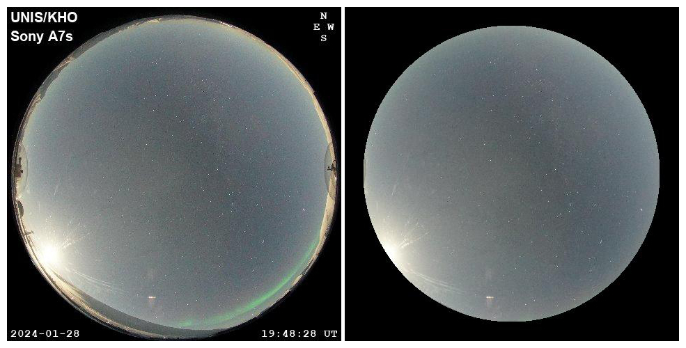
Figure 1 Example of a quicklook image (left). In a masked quicklook image (right), the lowest elevation angles and all metadata are blocked.

Figure 1 illustrates the difference between unmasked (left) and masked image (right). The masking excludes the lowest elevation auroral emission in this case. This type of auroral occurrence does not provide useful information on shapes or emission brightness. The masking further excludes nearby mountain slopes, neighbouring instrument domes as well as all meta data (date, time and compass), all of these being distractions for the manual labelling. Due to the masking, this example image was labelled as ClearNoAurora even though there is auroral activity very low in the southern horizon. Note that the classifier training was carried out with unmasked images; the classifier learns to ignore the areas not relevant for the classification.

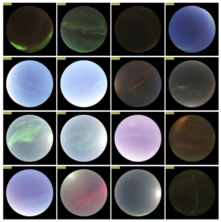
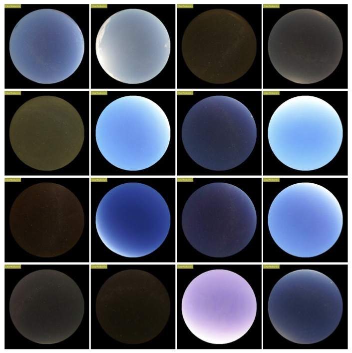
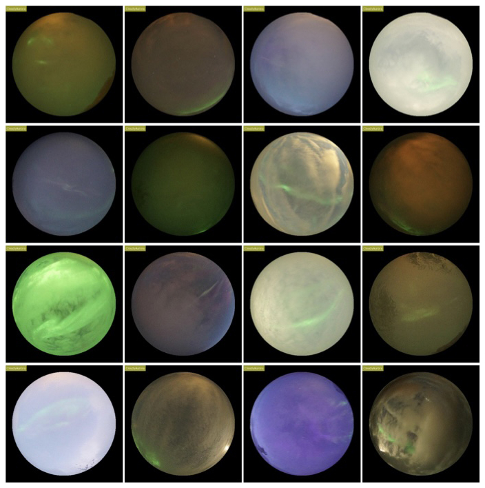
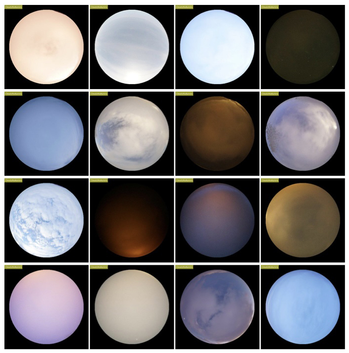
Because we discarded all images for which we were unable to provide a conclusive class, we were left with fewer images but with better confidence in labels. Four examples of ground truth training images from each class are shown in Fig. 2, from top to bottom: ClearAurora, ClearNoAurora, CloudyAurora and CloudyNoAurora. These examples demonstrate the variety of different sky illumination conditions. More examples of each class are included in Figs. A1–A4.

Figure 2 Sample images from the training set of ClearAurora (top row), ClearNoAurora (second row), CloudyAurora (third row), and CloudyNoAurora (bottom row). More examples in Figs. A1–A4 in Appendix A. The label in each image was assigned by our classifier.

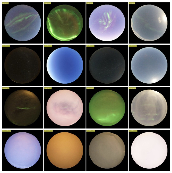
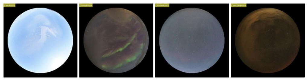
Figure 3 Examples of images in the Unclear class. From left to right: (1) frost on the dome but probably clear skies, (2) aurora and clouds/fog, just about $\mathrm{3}/\mathrm{8}$, (3) dim red emission band and high clouds, (4) clouds and probably red emission low in the horizon. The label in each image was assigned by our classifier.

Example images of the Unclear class are shown in Fig. 3. From left to right they were classified into ClearAurora, CloudyAurora, ClearNoAurora and CloudyNoAurora, respectively, but were manually moved to the Unclear class. In the first image the sky is probably clear, but the structure in the middle is formed by frost on the dome rather than aurora. The second image has clouds and aurora, but the larger regions appearing as clouds are probably condensation on the dome, which covers perhaps less than $\mathrm{3}/\mathrm{8}$. The third image shows a full field-of-view covered by high clouds. In addition, there is a faint band of red emission on the sky, so the sky is neither clear nor void of aurora. The fourth image displays light pollution illuminated clouds, but also some faint red glow very low in the horizon. As these images cannot be unambiguously assigned to any of sky condition classes, they were manually re-labelled as Unclear and removed from the ground truth.

Table 2 Numbers of manually labelled images throughout the iterative process of accumulating the ground truth (bottom). The bold text marks the numbers of images, which together comprise the ground truth.

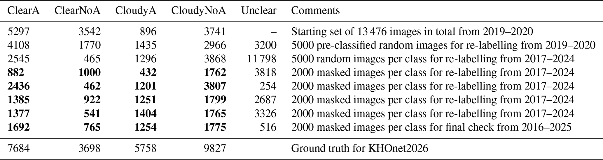
Table 3 Confusion matrix of the validation and test scores of KHOnet2026. The bold numbers indicate the numbers of correctly classified images. Percentage values (success rates) are given in scores of recall (last column) and precision (second last row). The bottom row shows the correct classification of an independent test set.

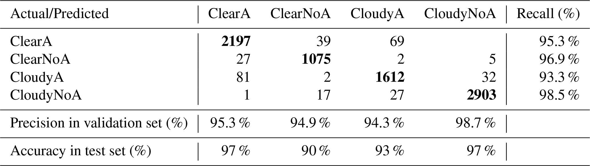
Table 3 shows the confusion matrix of our final classifier KHOnet2026 with class-specific accuracies in validation as well as the accuracies in testing with an independent dataset. Recall measures how many of the images in each class were classified correctly, while precision indicates how often the predicted classes were correct. The total number of images per class in Table 3 corresponds to 30 % of the ground truth images (bottom row in Table 2). The diagonal values describing correctly predicted classes are the highest. The classes ClearAurora, ClearNoAurora and CloudyNoAurora are well predicted, while the class CloudyAurora has the highest uncertainty. Notably, all score values in validation are over 93 %.

An independent test set was constructed by selecting 2000 random images per class from all classified data in 2016–2025. None of the images in the test set were used in training the classifier. This test set was then used to estimate the final classification error from the perspective of the (same) expert (bottom row in Table 3), and to examine which classes are confused with each other. The classes of ClearAurora and CloudyNoAurora had the highest success rates of 97 %. The ClearAurora images were mostly confused with the class of CloudyAurora in the test, while in validation this class also had some overlap with the ClearNoAurora class. These overlap cases include sky conditions with a little bit of cloud cover or only a small area of aurora or very faint auroral emission. The CloudyAurora images were detected with 93 % success rate in testing. They were typically confused with clear sky conditions with aurora, which is happens when the cloud cover is close to the half-sky value. The CloudyNoAurora were detected with 90 % success in the testing. These conditions were mainly confused with cloudy skies with a little bit of aurora.

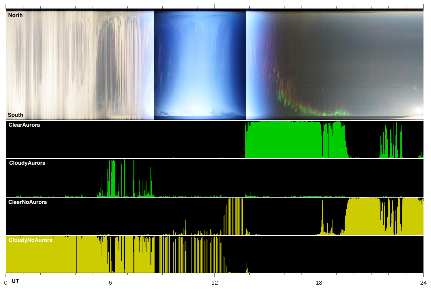
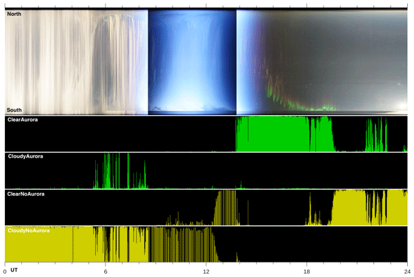
Figure 4 An example of the classification results in a keogram format. Top: a full day keogram of ASC images on 28 January 2024, north is to the top and south to the bottom of the panel. The noon is bracketed by changes in the expose time. Second: probability of ClearAurora, Third: probability of CloudyAurora, Fourth: probability of ClearNoAurora, and Bottom: probability of CloudyNoAurora. The class probabilities range from 0 at the bottom of each panel to 1 at the top of each panel, and the height of the colour bars indicate the probability of the class for each image.

An example day of the classification results is displayed in Fig. 4. The top panel shows the keogram of all images on 28 January 2024. In this format, the vertical centre column is extracted from each image to be stacked into a timeline. The panels below illustrate the probability of each class for each image as the height of the colour bar (green for aurora or yellow for no aurora). The morning is covered by moonlit clouds (high probability of CloudyNoAurora). Around noon there are two changes of the exposure time, and the sky brightness introduces some uncertainty on the sky conditions. The afternoon images contain red and green aurora (high probability of ClearAurora). The abrupt start of the high probability of ClearAurora seems to coincide with the change in exposure time, which can make auroral structures more visible in the images. In fact, individual images show auroral structures on clear skies already 1 min before the exposure change, and they are correctly classified as ClearAurora. The third panel shows the probability of CloudyAurora. It is only high in the morning, when there are some auroral structures in between the clouds. This is difficult to distinguish in the keogram format but is visible in individual images. Towards the end of the day (at about 20:00–24:00 UT) the sky is clear and no aurora can be seen. Correspondingly, the time period is high on the probability of ClearNoAurora. Animation of the individual images for this day can be viewed on the AuroraX Keogramist tool (https://aurorax.space/keogramist, last access: 28 September 2026).

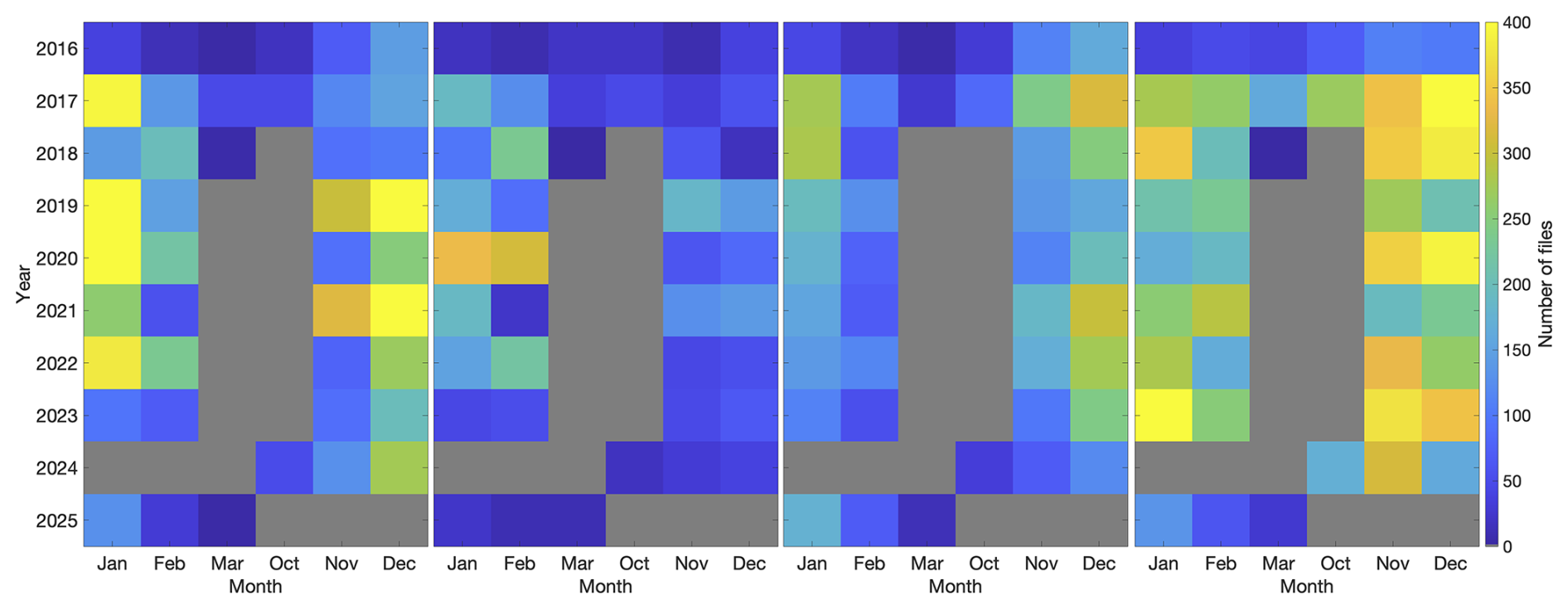
Figure 5 Distribution of the training data (ground truth, Partamies and Syrjäsuo, 2026) between years and months for all 4 classes left to right: ClearAurora (7684 images), ClearNoAurora (3698 images), CloudyAurora (5758 images), CloudyNoAurora (9827 images). Gray colour marks bins with no image files used in training the classifier.

Figure 5 shows the distribution of the images used in the training of KHOnet2026 (Partamies and Syrjäsuo, 2026). The panels from left to right separate the different classes: ClearAurora, ClearNoAurora, CloudyAurora, CloudyNoAurora. The gray colour marks the bins with no data. The highest monthly numbers are the December and January maxima of ClearAurora in the winter seasons of 2019–2020 and 2021–2022 (left panel). The lowest monthly numbers of training data are images for ClearNoAurora (second panel), which is the hardest class to find examples for. The most even distribution of training data was found for the CloudyNoAurora class (right panel), which also makes sense as every month would have some cloudy nights. Nonetheless, all years and all months of the core imaging season (November through February) are well represented in our training set. In the early years of imaging (2016–2017), also the months of March and October have been sampled. Furthermore, all classes of the ground truth include about 15 % of twilight images and images containing the Moon (about 30 %).

As each image could only be provided with one label – the one corresponding to the maximum probability – we examined the original probability distributions for individual images within each class. Intuitively, in the ClearAurora class, all images should have low probability values for the other classes. Within the class of CloudyNoAurora, 92 % of images had a probability value of 0.9 or higher. The same threshold resulted in 85 % of images in ClearAurora, 74 % in ClearNoAurora and 74 % in the CloudyAurora class. These findings are in agreement with the numbers of false predictions seen in the confusion matrix (Fig. 3).

We used a desktop computer with an NVIDIA GeForce RTX 4090 Graphics Processing Unit (GPU) for training the classifier. For our initial experiments with GoogLeNet, the training took 2–5 min depending on the choice of hyperparameters. With InceptionV3 as the starting point for transfer learning – which produced the final classifier KHOnet2026 (https://github.com/UNISvalbard/KHOnet2026/, last access: 28 September 2026) – the training took about 12 min. The classification of all images from the beginning of 2016 to the end of 2025 took 14.2 h, or roughly 6 ms per image, including the time needed for file reading. The classifier development was done using Matlab (R2025b) with GPU-acceleration, but we also deployed a prototype real-time classifier at KHO using PyTorch (Paszke et al., 2019). Using an older computer with no GPU acceleration, the classification of a new thumbnail image takes roughly 0.1 s including reading image data from a file server and annotation of the output image. With this processing speed, we can easily classify images in realtime even with a higher imaging rate than the current 12 s.

4 Results

4.1 Classification results

Training of a CNN is an iterative process (non-linear optimisation) and there are several hyperparameters that can be adjusted or kept fixed during the training. In our case, the aim was to obtain accuracies of the order of 95 % for each class. After each training epoch, the performance of the classifier-in-training was evaluated using a validation set: an accuracy plateau above 90 % was usually reached quite rapidly, and therefore it is likely that we could fine-tune the parameters in the learning algorithm to obtain improved results or even faster convergence to reduce the computation time. We chose to use a straightforward grid-search method where we varied hyperparameters within a specified range, and then selected the classifier with a set of hyperparameters that performed best. From the point of view of long-term analysis in auroral research, we consider a difference between 95 % and 96 % correct classification insignificant, but one of the classes being several percentages lower than others can become a significant statistical bias. Our set of labelled auroral images (ground truth from the bottom row of Table 2) can be used as a reference set for further development and experiments. An obvious possibility would be to use the training set with self-supervised learning to increase the number of labelled images, which may lead to more accurate results.

For the main analysis we used data from the Sony ASC since 2016. However, its predecessor DSLR (Nikon D80 with an all-sky lens) was operated at the same time in January and February 2016. We used KHOnet2026 to classify previously unseen DSLR images from the overlapping time range to compare the classification results. The cameras were not perfectly synchronised, but the time differences varied from 0 to 15 s with a median of 7 s. Simply counting on time instances when the maximum probability was given to the same class, we obtained matching values for 96 % images in the class of ClearAurora, 97 % for images of ClearNoAurora, 92 % for images of CloudyAurora, and 94 % for images of CloudyNoAurora. These results did not change more than 0.5 % when the time difference tolerance between the images from the two cameras was limited to 10 s instead of 5 s, suggesting that the discrepancies were due to instrument properties (such as white balance) rather than evolving sky conditions.

According to a manual inspection of about 1000 randomly selected DSLR images from each class, KHOnet2026 correctly classified 90 % of the images in the ClearAurora class (785 images), 65 % of the images of ClearNoAurora class (450 images), 86 % of the images of CloudyAurora (632 images) and 94 % of the images of CloudyNoAurora (884 images). For all but the CloudyAurora class, the ambiguous images of the Unclear class were the largest group of the “wrongly classified” images. Any data with technical problems have been excluded. As an older and less sensitive camera system, in many cases it was difficult to judge whether there was aurora or not, and particularly whether the sky was actually clear or not. The most important classes (those including aurora) were reasonably well detected. The largest confusion in the CloudyAurora class was with images of CloudyNoAurora. This was largely due to a combination of red background sky with moonlight clouds, which was interpret as red auroral emission in between the clouds. The classification accuracy can be improved by adding manually labelled DSLR images to this re-labelled set of data, and then training a classifier with the more specific ground truth. This would extend our time series of auroral and nighttime cloudiness occurrence by another 7 years.

4.2 Properties of long-term auroral and cloud observations

To analyse the long-term evolution of auroral and cloud occurrence, we have taken the class of maximum probability to be the correct auroral class for each individual image. The maximum probability class was given a value 1, while other classes were set to zero. The temporal evolution of these values then gives the occurrence of each class as a function of time. In the following, we focus on examining the Magnetic Local Time (MLT) distribution of auroral occurrence (AO) and cloudiness occurrence (CO) for the full dataset from the beginning of 2016 until the end of 2025. For seasonal and annual variability, we also show monthly and yearly binned occurrences. The occurrence values are normalised by the total number of images in each bin. This normalisation allows us to directly compare the occurrences of aurora, cloudiness and clear skies. AO is defined as a combination of classes of ClearAurora and CloudyAurora (∼ 2 million images) to show an auroral evolution as it is seen from the ground. We cannot determine AO when the clouds block the visibility to the ionosphere, which reduces the number of samples in the statistics. CO only counts for cloudy skies without aurora (∼ 5 million images). MLT is estimated as UT +2.5 h.

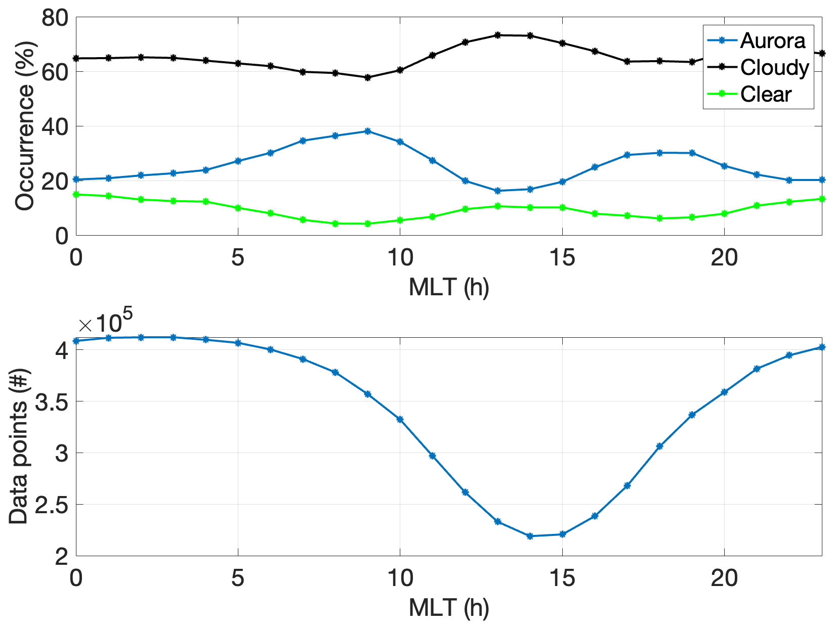
Figure 6 MLT distribution of the occurrence of aurora (blue), cloudy (black) and clear skies (green) in the entire dataset. Hourly occurrence is normalised to the total number of observations per bin, which is plotted in the bottom panel. Svalbard MLT is estimated as UT +2.5 h.

Figure 6 shows the hourly binned MLT distribution of AO (blue), as well as an occurrence of cloudy (black) and clear skies (green). The percentages of the three classes sum up to 100 % in each bin. The lowest occurrence is for the clear skies without aurora, which happens 5 %–15 % of the time. AO varies between 15 % and 40 % with maxima at 09:00 MLT and 17:00–19:00 MLT and minima at 13:00–14:00 MLT and 23:00–01:00 MLT. Cloudy skies, however, are seen by far most often: 60 %–75 % of the time with a maximum occurrence in early afternoon (13:00–14:00 MLT). The above mentioned behaviour of occurrence rates of AO, clear and cloudy skies is very similar for all individual years in our dataset.

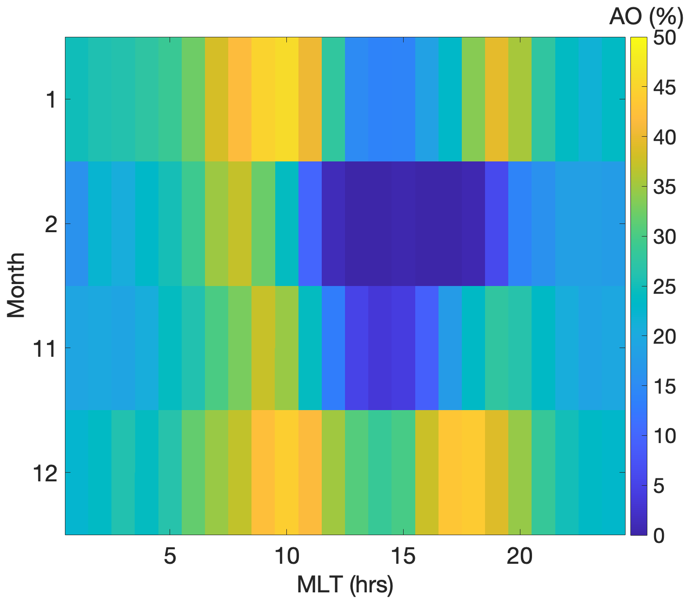
Figure 7 Auroral Occurrence (AO, colour-coded) as a function of month and MLT. The bin size is 1 h and the data are normalised to the total number of images per bin.

A more detailed variability of AO is shown in Fig. 7, which presents the auroral occurrence as a colour coded heat map as a function of MLT and month. The number of images during the daytime hours strongly depends on the month. In January (1) and December (12), AO describes the true occurrence of aurora, while in February (2) and November (11), the low number of images around midday presents a low chance for aurora and therefore a low AO despite the normalisation. The double-peak MLT distribution seen in Fig. 6 is present in January, November and December, while the increasing daylight in February coincides with the late afternoon maximum so that only the morning MLT maximum is visible. January and December stand out as the months with highest AO. December further shows the most persistent AO throughout the day.

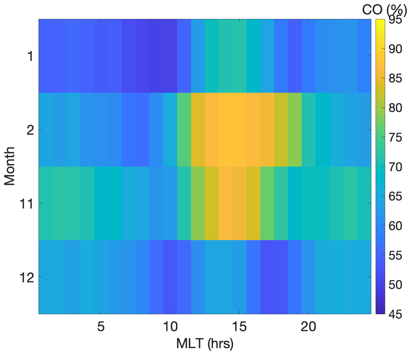
Figure 8 Cloud occurrence (CO, colour-coded) as a function of month and MLT. The bin size is 1 h and the data are normalised to the total number of images per bin.

A similar distribution is shown for the cloud occurrence (CO) in Fig. 8, which only includes the images of cloudy skies without auroral emission. These conditions are present at least 45 % of the imaging time throughout our dataset. The least cloudy month is January. The cloudiness maximum in the afternoon (∼ 15:00 MLT) coincides with the time of most daylight in February and November, while the lowest cloudiness values around 10:00 MLT and 17:00–18:00 MLT take place during dark hours in January and December. November stands out as the cloudiest month over Svalbard.

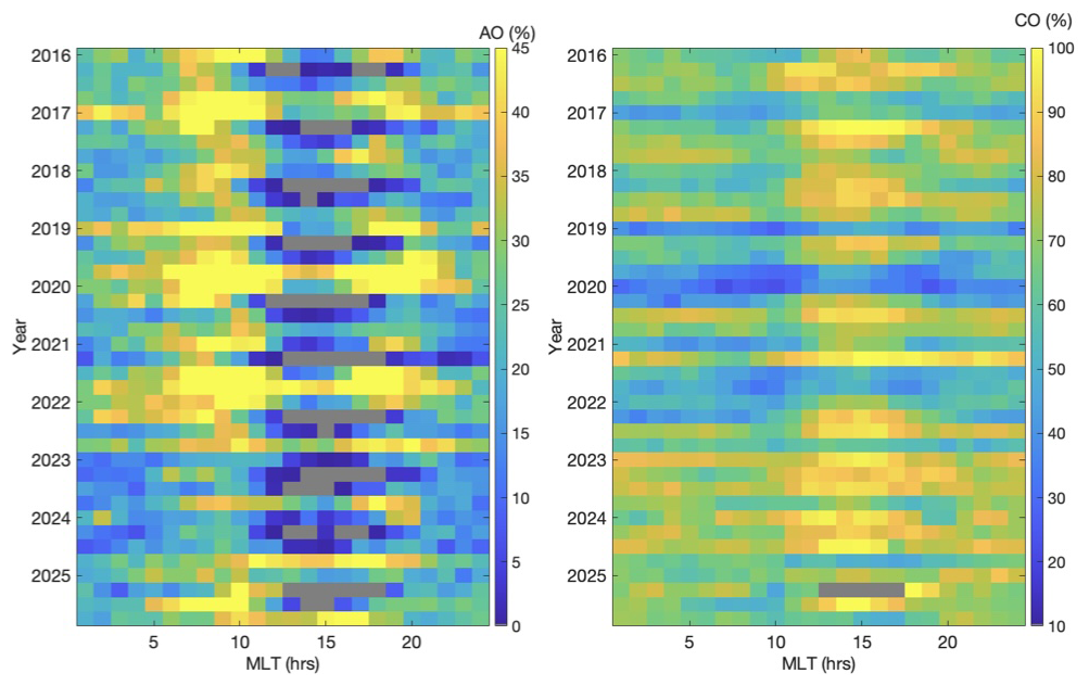
Figure 9 AO (left) and CO (right) as a function of month and MLT for the entire dataset, 2016–2025. The bin size is 1 h. Months of January–February and November–Dece,ber are included for all years. The data are normalised to the total number of images per bin. The gray colour marks the empty bins.

In order to see the inter-annual variability, Fig. 9 displays the monthly MLT distributions of AO (left) and CO (right) for all years from 2016 until 2025. Besides a few exceptions, the monthly averaged MLT distribution of AO shows mild auroral activity (10 %–25 %) around MLT midnight. The highest AO values of nearly each month are seen in the late morning hours at about 07:00–11:00 MLT, as well as in the premidnight hours of 17:00–21:00 MLT (less pronounced). The year of lowest AO in our dataset was 2023, while the most persistently high AO happened in 2019, closely followed by years 2021 and 2022. Compared to CO on the right hand side, it is obvious that the main factor controlling AO is the cloudiness, as the lowest AO year was the year with the highest cloudiness in 2023. Correspondingly, during the years of highest AO in 2019, 2021 and 2022, the cloudiness was low compared to other years.

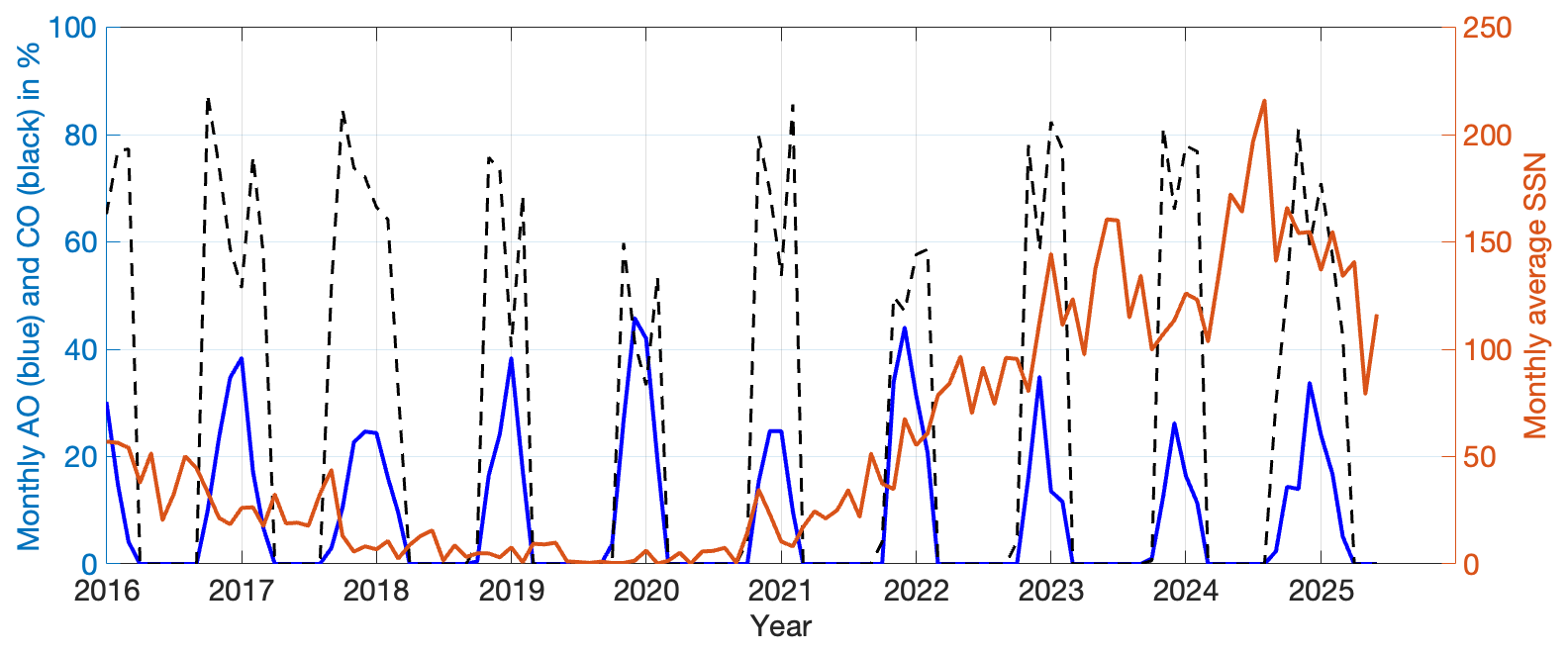
Figure 10 Monthly AO (blue) and CO (dark dash) together with the monthly average sunspot number (SSN, in red) for the entire dataset from early 2016 to early 2025.

To illustrate the lack of obvious solar activity effect on the Svalbard auroral occurrence, Fig. 10 shows the monthly AO (blue) and CO (dark dash) variability for our entire dataset. As a comparison, we have plotted the monthly averaged total sunspot number (SSN) in red (Clette and Lefèvre, 2015). Summer months do not have AO or CO occurrence values in our dataset, while SSN is continuous. Compared to the slow SSN variation, the monthly AO values do not have a similar trend. The high AO values rather correspond to low monthly CO values without an obvious modulation from the solar cycle phases. The years of 2019 and 2022 have AO values peaking at about 40 %, while SSN is well under 20 for 2019, and moderately high but less than 100 for the winter months of 2022. In 2021, AO is lower than in 2019, although SSN has started to increase. A more detailed regression analysis may reveal some solar cycle dependence of the auroral occurrence, but that will require a much longer time series of image data than what we currently have analysed. This examination is therefore left for the future.

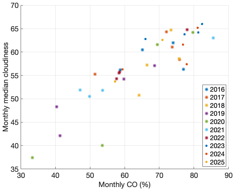
Figure 11 Comparison between monthly CO values and monthly cloud sensor measurements. Different years can be distinguished by colours and markers as shown by the legend.

To provide a comparison between our CO results and an independent estimate of cloudiness, we include measurements from a co-located cloud sensor (Aruliah and McWhirter, 2025). The two instruments have been operating in the same time frame. The cloud sensor measurements include the sky and sensor temperatures, and their difference is called clarity. While low clarity values are indicative for cloudy conditions, the high clarity values are a signature of clear skies. The clarity values have been shown to reliably describe the total cloudiness when a location-specific threshold is applied (Marocco, 2024). To compare with the monthly CO, we calculated monthly median values of 100-clarity without any threshold values, which we call “cloudiness”. This value then gives a positive correlation with CO, as shown in Fig. 11, with the correlation coefficient of 0.86. It is worth noting, however, that the cloudiness value of e.g. 60 is not the same as 60 % CO, because the two measures are inherently different. The values for different years are differentiated by the colours and the markers seen in the legend to illustrate how the scatter is distributed across the data. Taken into account that the two datasets are generated in very different ways, their agreement at a monthly level suggests that the classification recognises the cloudiness well. The scatter is likely to arise from the low values of total cloudiness (less than $\mathrm{4}/\mathrm{8}$) and the cloudiness with identifiable aurora, which are not accounted for in CO.

5 Discussion

5.1 Auroral classifier – remarks and future work

We carried out our experiments using supervised learning where the classifier's performance depends greatly on the quality of the training data. Finding representative images for each category was a major effort, during which we had to adjust our approach several times and consequently perform several rounds of manual labelling. We consider the accuracy of image classification with KHOnet2026 sufficient for long-term auroral studies, and for providing a cleaner dataset for more detailed auroral investigations. A visual inspection of the classification results for one day (Fig. 4) suggests that we could also use the classification results to study auroral activity at individual image level, perhaps with some additional post-processing of time series. One very important aspect of our training set is that the ground truth images will allow easy comparison between different classification methods in future. These images also provide a good starting point for further development of the pruning or analysis methods.

In general, one should have an equal number of samples from each class for the training of a classifier. We had clearly fewer images in the ClearNoAurora class of our training set than in the other classes for the simple reason that in most of our clear sky conditions there is some aurora visible somewhere in the all-sky field-of-view. For auroral studies, the central field-of-view is often considered the region of interest as the effective spatial resolution at auroral heights is highest in the centre of the image. Thus, we chose to mask the lower elevations in this study, as shown in Fig. 1. Ignoring lower elevations in our training set images improved the balance of image numbers per class, but did not fully even it out. We therefore carried out a quick experiment where the number of images from other classes was reduced to the level of samples in the ClearNoArurora class. As a result, the classification accuracy become worse. Rather than continuing with manual labelling efforts, we think the next logical step would be to employ self-supervised learning, or perhaps, semi-supervised learning to significantly increase the number of the labelled images.

One particularly confusing condition for the ClearNoAurora class is the phenomenon called Red Sky Enigma (Lloyd et al., 2005), where the sunlight reaches Svalbard through a double reflection on the polar stratospheric clouds during the polar night. It causes the background sky to turn red, which may easily be confused with auroral red emission or light polluted orange clouds. There are images of these conditions in the training set, but the number of them is limited, because the phenomenon does not take place every winter and not for many days at a time. The combinations of the red sky with cloud cover, twilight and aurora are therefore not well-taught to the classifier.

Other confusing sky conditions are when the images contain just too much or just too little clouds or barely detectable aurora. This “gray zone” was intentionally left out of the training data, which means that the number of these images will largely determine our classification error. During the dawn and dusk the background sky can be so bright that it is not possible to tell, even by a trained human expert, if the sky is clear or cloudy. These images end up in the same “gray zone” category (the Unclear class) by a human expert but will be assigned to one of the other classes by a CNN classifier. If the classifier judges these low-contrast conditions as cloudy more often than not, this could lead to a bias towards cloudiness in our dataset. This was tested by excluding the twilight conditions (the Sun above −12° below the horizon) and the moon above the horizon with illumination larger than 50 % from our dataset. As a result, CO and clear skies were reduced by 7 % and 3 %, respectively, while AO was increased by 6 %–7 %. However, the diurnal behaviour of AO, CO and clear skies (seen in Fig. 6) still persists. The drawback of this test is that the total number of images decreased by nearly 50 %. Because the reduced dataset shows the same diurnal evolution, we have included the twilight and moon up conditions in our analysis, but added the solar elevation angle, the moon elevation angle and illumination in the published classification data files to facilitate the data reduction that best fits the purpose of any future study.

In addition to cloudiness, real image data also contain technical problems, such as fog or snow on the dome, people or artificial lights in the images, which have all been excluded from the training of the classifier but have been assigned to one of the classes in the analysis of the entire dataset. However, as the high classification accuracy suggests, these type of confusing conditions do not represent a large amount of data.

No matter how carefully the ground truth has been constructed, there will always be biases. McKay and Kvammen (2020) provide a thorough discussion on the challenges of constructing a non-biased training set. In our study, perhaps the largest bias comes from the fact that all manual labelling was performed by only one of the authors. Albeit this process extended over many years and several iterations aided by pre-labelled images, our ground truth is still just one expert's subjective view on the classes and class boundaries.

Combining the machine learning with pixel-based intensity approach (Yamauchi and Brändström, 2023) to detect the local auroral brightenings in the pruned dataset could be a possible approach for future studies. From the methodology point of view, there are also other alternative classifier types, which may further improve the results. In particular, recent research has introduced Vision Transformers (ViT, Jamil et al., 2023) that would be worth testing on auroral image classification.

Comparing our methodology with earlier studies in auroral image classification, our approach is similar to the works by e.g. Kvammen et al. (2020) and Nanjo et al. (2022). The main difference is that we prefer to leave the analysis of image content to a separate follow-up step. Our choice is based on the fact that we cannot reliably describe the auroral shapes except in broad terms, and one auroral image often includes several types of aurora (arcs, patchy, diffuse, unidentified shapes etc.). In our opinion, the different auroral classes should be learned from the data in a way that avoids human bias as much as possible in handling these uncertainties. Our experiments with unsupervised learning (Partamies et al., 2024) and the successful use of self-supervised learning by Johnson et al. (2024) are encouraging steps to this direction. Another difference between our approach and that of Kvammen et al. (2020) and Nanjo et al. (2022) is that we allow the Moon and twilight in all our classes. This keeps the classes very broad and serves as an initial data pruning method, from which the results can be repurposed for studies with many different criteria. Finally, our manual labelling has been performed in an iterative way, rather than in one go, which has allowed us to follow the evolution of the classification process and discuss its challenges, letting the procedure, purpose and implementation mature over time.

5.2 Statistical occurrence rates of clouds and aurora

The cloudiness level is very high in our dataset, even though images in the CloudyAurora class are not included in CO. Fortunately, the least cloudy months and hours in the dataset were during the darkest hours and therefore well captured. The high level of cloudiness and its small diurnal variability in Svalbard was already discussed by Partamies et al. (2001). Their data only covered two winter seasons (1996–1997 and 1997–1998) with more images from the MLT morning than evening hours. In our statistics, it is particularly the months of January through to March when the morning MLT hours have been more often clear than the evening hours. A longer-term analysis of total cloudiness over Svalbard by Bednorz et al. (2016) also concluded on high values (around 60 %) and little variability, which is in agreement with our results. They further showed an increasing trend in the winter season cloudiness in the time frame of 1981–2010. Our dataset is too short for a long-term trend analysis but it can provide more robust nighttime cloudiness information in the future. To get an independent estimate of the cloudiness in the time frame of our dataset, we used data from a co-located cloud sensor as a validation for our classification results. The two datasets are in a very good agreement suggesting that our classification does a good job in detecting cloudy skies.

On average, the auroral occurrence is about 25 % of all imaging time, while clear skies without aurora is seen about 10 % of the imaging time. This suggests that auroral observations are mostly limited by cloudiness. In the long-term perspective, Svalbard AO does not correlate with the solar activity, but rather shows a nearly constant percentage throughout the solar cycle. A similar conclusion was presented by Pulkkinen et al. (2011) in their study of electrojet and visually determined auroral activity during the solar cycle 23. According to the previous studies (Nevanlinna and Pulkkinen, 2001; Partamies et al., 2014), a solar cycle variation appears in the evolution of auroral structures and their absolute intensities, which are driven by enhanced solar wind and geomagnetic activity. The lowest annual AO (16 %) in our dataset was observed during the year 2023, not because of the low solar activity but because of exceptionally cloudy winter months (78 %). The highest AO of 33 % was observed during year 2019, which was a year of low solar activity, but a year with an exceptionally low cloudiness (54 %).

AO correlation with magnetic activity at auroral oval latitudes in Tromsø, Northern Norway, was documented by Nanjo et al. (2022). Their analysis covered the years of 2011–2020, which is partially the same data range as ours (2016–2025). They found a peak AO year to be 2015 in the declining phase of the solar cycle, and their monthly AO maxima to took place in the autumn and spring towards the equinoxes. In contrast, the highest Svalbard AO values are seen around the winter solstice, while equinox times are contaminated by daylight and already outside the core imaging season in Svalbard. The AO percentages reported by Nanjo et al. (2022) are higher than ours by more than 20 %. This is due to the different normalisation, which in their case excludes the cloudy conditions, while we use the number of all images per bin. Our choice of normalisation allows us to compare AO and CO to each other, as well as compare our results to the earlier visual inspection studies by Nevanlinna and Pulkkinen (1998, 2001).

Svalbard AO most frequently maximises in the pre-noon and early evening MLT hours, while the post-noon and midnight show the lowest probability. This distribution remained the same throughout the inspected years. While there may be modulation of the diurnal distribution of AO by the level of magnetic activity related to the expanding and contracting auroral oval, a detailed examination of that effect is left for future studies.

Overall, having an automatic image classification method in operational use allows us to revisit this long-term overview of AO and CO on regular basis. It facilitates the use of more efficient data searching routines and much more efficient further analysis of the images containing aurora. As Svalbard is also a home for frequent measurement campaigns (with sounding rockets and European Incoherent Scatter (EISCAT) radar experiments), statistical results will provide a helpful background for planning optical measurements with least probable cloud contamination.

6 Conclusions

We report on the first operational auroral image classification routine, KHOnet2016, for pruning full-colour data into the classes of Aurora, NoAurora and Clouds without excluding or separating twilight and moonlit conditions, and with the inclusion of both nightside and dayside aurora. To the best of our knowledge, only two other classification methods have so far been employed in operational use (Nanjo et al., 2022; Yamauchi and Brändström, 2023), both with different purposes and approaches. Unlike earlier studies, we analyse the cloud occurrence as well as the auroral occurrence. The Svalbard image dataset also carries a special feature of including images of the dayside aurora during the polar night, when optical observations can be made 24/7. The inclusion of daytime aurora poses an additional classification challenge by expanding the range of possible sky conditions. Nonetheless, KHOnet2026 reaches an average accuracy of about 95 % for all classes.

Our 10-year-long dataset shows auroral occurrence (AO) about one fourth of the time and cloudiness nearly $\mathrm{2}/\mathrm{3}$ of the time, while clear skies without aurora only occur about 10 % of the time. Monthly averaged AO does not correlate with the solar activity at these high latitudes, but is rather modulated by the cloudiness. As a major part of our sky conditions were cloudy, we sanity checked our cloudiness with a co-located cloud sensor data and found them in a very good agreement with a correlation coefficient of 0.86. Our results suggest that the clearest skies, and therefore most aurora, can be seen in January. The least favourable aurora month is November. This type of information can be used in planning for future measurement campaigns. More importantly, an automatic classification of all past auroral image data (8 million images in this study) will allow further analysis of aurora types in a much more efficient way, and will help the analysis of data from any instrument hosted at KHO.

Appendix A: Additional examples of ground truth

Figures A1–A4 display additional ground truth images of each class.

Figure A1 Ground truth images of ClearAurora.

Figure A2 Ground truth images of ClearNoAurora.

Figure A3 Ground truth images of CloudyAurora.

Figure A4 Ground truth images of CloudyNoAurora.