Globally- and hemispherically-integrated Joule heating rates during the 17 March 2015 geomagnetic storm, according to physics-based and empirical models

Joule heating is a primary energy dissipation mechanism of the solar wind in the Earth's upper atmosphere. However there are large discrepancies in the computation of Joule heating between models. In this study, we perform a comparison of the Joule heating rates between two of the most commonly used physics-based Global Circulation Models (GCM) of the Earth's upper atmosphere: the Global Ionosphere/Thermosphere Model (GITM) and the Thermosphere-Ionosphere-Electrodynamics General Circulation Model (TIE-GCM). Both GCMs are externally driven by models that provide the specification of high-latitude electric fields as well as auroral precipitation. In this study, each model is driven by two different specifications of high-latitude electric fields, namely the Weimer 2005 and the Assimilative Mapping of Ionospheric Electrodynamics (AMIE) models. Several empirical formulations are also commonly used to estimate Joule heating rates as a function of various indices of solar and geomagnetic activity; a further comparison is performed between these empirical formulations and the GCMs. We find that the empirical formulations generally give lower estimates of Joule heating rates compared to both GCMs, GITM and TIE-GCM. We also find that TIE-GCM provides lower estimates of the heating rates compared to GITM when the Weimer 2005 model is used as driver, whereas TIE-GCM and GITM give rather similar estimates when the AMIE model is used, with TIE-GCM occasionally giving higher estimates. Estimates of Joule heating rates separately for the two hemispheres indicate that higher Joule heating rates are observed in the Southern Hemisphere when the Weimer model is used, both in GITM and TIE-GCM. However, when the AMIE method is used, higher Joule heating rates are calculated for the Northern Hemisphere. The comparisons between the two Global Circulation models and the empirical models are discussed.

1 Introduction

During geomagnetic storms, Joule heating is known to be the dominant solar wind energy dissipation mechanism. Joule heating maximizes in the lower thermosphere-ionosphere (LTI) region, within the 100–200 km altitude range, where current density and conductivity (Pedersen and Hall) maximize (Huang et al., 2012; Baloukidis et al., 2023). The quantification of Joule heating is a subject of intense research, as it is critical in determining the structure and evolution of the Lower Thermosphere-Ionosphere, and is responsible for a number of effects of societal importance, such as for determining atmospheric drag and predicting the resulting deorbiting times of satellites and space debris within this region (Palmroth et al., 2021; Sarris et al., 2023a). For example, the loss of 40 Space-X's Starlink satellites in February 2022 is thought to have been caused by an underestimate of the enhancement of thermospheric neutral density that resulted from enhanced Joule heating during a moderate geomagnetic storm (Dang et al., 2022; Zhang et al., 2022b; Hapgood et al., 2022). It is for this reason that quantifying the heating rates is critical in order to accurately determine satellite drag and orbital lifetime estimations.

Whereas the physics of the collisional processes leading to Joule heating is well understood and is captured in Global Circulation Models (GCMs) of the ionosphere-thermosphere (IT) system, the quantification of Joule heating is still largely unknown, and large discrepancies appear between different models and estimation methodologies (Palmroth et al., 2005; Rodger et al., 2001). This is in part because the exact quantification of Joule heating requires the simultaneous and co-located measurement of all relevant parameters that are involved in the calculations of conductivity, electrical currents and fields, and in part because an unknown amount of Joule heating is related to small-scale or sub-grid variability that can not be captured by current models. Also contributing to the above uncertainty, the lower thermosphere-ionosphere (LTI) region, where Joule heating maximizes, is the least sampled of all atmospheric regions (see, e.g. Sarris et al., 2023a, and references therein): the altitude range from ∼100–200 km is too high for balloon experiments and too low for Low-Earth Orbit (LEO) satellites, due to the large air drag. Thus, the majority of available measurements for this region comes from ground based observatories, such as Incoherent Scatter Radars, and very few in-situ space missions, such as the Atmosphere Explorers of the early 1980s. Measurements from the above are used in formulating empirical models of the upper atmosphere, such as the International Reference Ionosphere (IRI) (Bilitza, 2018), NRLMSISE-00 (Picone et al., 2002) and the Horizontal Wind Model (HWM) (Drob et al., 2008). Furthermore, physics-based global circulation Models (GCM), such as the Global Ionosphere/Thermosphere Model (GITM) (Ridley et al., 2006) or the National Center for Atmospheric Research (NCAR) Thermosphere-Ionosphere-Electrodynamics General Circulation Model (TIE-GCM) (Qian et al., 2014) simulate the energetics, dynamics and chemistry of this region. However, there are great discrepancies in describing the basic state of the LTI between empirical models and physics-based models, such as neutral temperature and density, which is largely due to the uncertainty in estimating the amount of Joule heating in the LTI.

Among physics-based models, GITM and TIE-GCM are widely used by the upper atmosphere scientific community. Both are 3D gridded numerical models that are used to simulate the state of the thermosphere and ionosphere in response to external driving by solar wind conditions. GITM and TIE-GCM are both based on a set of equations that describe the physical processes that occur within the thermosphere and ionosphere, such as radiation, convection, and dynamical forcing. From the outputs of these models, which include all essential variables or geophysical observables of the thermosphere and ionosphere, Joule heating can be directly computed at each model grid point.

Together with the above physics-based models, a number of empirical formulations have been derived as proxies of Joule heating, driven by solar and geomagnetic conditions. For example, Joule heating has been found to be closely related to the AE and AL indices (see, e.g. Perreault and Akasofu, 1978; Akasofu, 1981; Baumjohann and Kamide, 1984; Ahn et al., 1983, 1989; Richmond et al., 1990; Cooper et al., 1995; Lu et al., 1995, 1998). Seasonal and hemispherical differences have been examined as well to establish a more accurate relation between Joule heating and the geomagnetic indices (Nisbet, 1982; Lu et al., 1998). Further to the above, Chun et al. (1999) estimated Joule heating with a quadratic fit to the Polar Cap (PC) index, whereas Knipp et al. (2005) expanded on the work of Chun et al. (1999) by proposing a formula that is based on both the PC and the Disturbance Storm Time (Dst) indices; and Weimer (2005) calculated Joule heating empirically, based on a model of Poynting flux that is derived using measurements of the Dynamics Explorer 2 satellite. It is noted that most of the above empirical formulations do not take into account the effects of neutral winds, which are known to impact Joule heating significantly (see, e.g. Lu et al., 1995; Emery et al., 1999).

Empirical models are often designed to describe large-scale climatology and can thus underestimate the real-time magnetospheric energy input. Such differences between empirical models and observations have been discussed extensively in the literature (see, e.g. Cosgrove and Codrescu, 2009; Cosgrove et al., 2011). Various data assimilation methods have been developed which can be used to mitigate the discrepancy, e.g. the standard AMIE procedure (Richmond and Kamide, 1988) and methods like SECS (Amm, 1997), Local Divergence-Free Fitting (LDFF) of SuperDARN observations (Bristow et al., 2016) and Lattice Kriging (Wu and Lu, 2022). Data assimilation methods are used to replace the empirical high-latitude drivers in GCMs, resulting in higher levels of variability, and enhanced Joule heating. These usually show a better agreement with observations. Some examples of data-driven modeling include the studies by Lu et al. (2020), who performed extensive comparisons between simulation results from TIE-GCM using AMIE as a driver, and Lu et al. (2023), who also used TIE-GCM using the Lattice Kriging method to derive their high-latitude auroral and convection patterns.

In the following, Joule heating estimates are calculated and presented based on simulation results of the solar storm of 17 March 2015, the largest geomagnetic storm of solar cycle 24, which is also known as St. Patrick's Day 2015 storm. As part of this study, globally integrated Joule heating rates are calculated in both GITM and TIE-GCM, and are compared against estimates obtained from various empirical formulations. GITM and TIE-GCM simulations are performed using both the Weimer 2005 empirical high-latitude electric field model (Weimer, 2005) and the AMIE data assimilation method (Richmond and Kamide, 1988) as drivers. It is noted that the integration of other available electric field data assimilation models such as those listed above (i.e. the models by Richmond and Kamide, 1988; Amm, 1997; Bristow et al., 2016, and Wu and Lu, 2022) with TIE-GCM and GITM was not available to the authors at the time of this study, and is not considered herein. The integration of the above data assimilation methods as drivers of commonly used GCMs is a topic of future research. Joule heating estimates are presented as time series over the course of St. Patrick's Day 2015 storm. Together with the time series of the evolution of Joule heating during the storm, the cumulative globally integrated Joule heating is compared as calculated by each model. Furthermore, hemispherically-integrated Joule heating rate estimates are compared between GITM and TIE-GCM.

This paper is organized as follows: Sect. 2 presents details of the GITM and TIE-GCM, including their external drivers, and describes the derivation of Joule heating in both models. Section 3 presents the results of the implementation of the simulations for St. Patrick's Day 2015 storm as well as the resulting Joule heating as obtained from various empirical formulations. Section 4 discusses the results, highlighting potential causes of the observed discrepancies. Finally, Sect. 5 summarizes the conclusions of this work.

2 General Circulation Models

2.1 The Global Ionosphere-Thermosphere Model (GITM)

GITM is a non-hydrostatic global circulation model that has been developed in order to simulate the energy balance, chemistry, and dynamics of the Earth's ionosphere and thermosphere (Ridley et al., 2006; Vichare et al., 2012; Deng et al., 2019). It has also been used to simulate planetary upper atmospheres (Bougher et al., 2015). GITM simulates the state of the mutually coupled ionosphere and thermosphere at altitudes from 100 to ∼600 km. It solves the coupled continuity, momentum and energy equations of neutrals and ions. The continuity, momentum, and energy equations in GITM have realistic source terms. Furthermore, GITM solves for the horizontal advection for both ions and neutrals using a 2nd order Rusanov solver that makes no smoothing approximations near the poles. The complete vertical momentum equation is solved using the AUSM solver (see, e.g. Ullrich et al., 2010), with each species having individual vertical momentum equations and velocities with diffusive coupling terms that limit the inter-species flows in the lower regions of the model where the eddy diffusion is large. The vertical grid spacing is typically around 0.3 times the scale height of the dayside low latitude thermosphere and is set at the start of the simulation. The low latitude dynamo is described by Vichare et al. (2012). The chemistry is solved for implicitly, allowing for rapid variations in the individual species densities. The electron and ion temperatures are solved for using semi-implicit schemes, as described by Zhu and Ridley (2016), allowing for non-steady-state evolution of both. Each neutral species has a distinct vertical velocity, with a frictional term linking the velocities. Ion species in GITM include: O⁺(⁴S), O⁺(²D), O⁺(²P), ${\mathrm{O}}_{\mathrm{2}}^{+}$, N⁺, ${\mathrm{N}}_{\mathrm{2}}^{+}$, and NO⁺ whereas neutral species include: O, O₂, N(²D), N(²P), N(⁴S), N₂, and NO. A key advantage of GITM is that it is capable of employing a versatile, non-uniform grid, with variable resolution in both altitude and latitude, as opposed to a pressure grid that is commonly used in other thermosphere codes. The vertical grid spacing is less than 3 km in the lower thermosphere, at altitudes from 100 to ∼250 km, whereas it is over 10 km in the upper thermosphere, at altitudes from ∼250 to 600 km. The ion momentum equation is solved with the assumption of a stable state, while accounting for the pressure, gravity, neutral breezes, and external electric fields. Several high-latitude ionospheric electrodynamic models have been used as external drivers of GITM; these include, among others, the Assimilative Mapping of Ionosphepric Electrodynamics (AMIE) approach (Richmond and Kamide, 1988), the Weimer model (Weimer, 2005), and the Ridley et al. electrodynamic potential pattern (Ridley et al., 2000). GITM model runs are initiated in a number of different ways, such as (1) utilizing an ideal environment in which the user inputs the density and temperature at the base of the atmosphere; (2) using MSIS (Picone et al., 2002) and International Reference Ionosphere (IRI) (Bilitza, 2018); and (3) starting from a prior run. In the present study, the second of the above initialization approaches is followed.

Using the geophysical parameters that are produced as outputs of GITM, Joule heating can then be estimated. These estimations require in addition the computation of electrical current, J, and Pedersen conductivity, σ_P. The equations that are used in the estimations of the above heating rates are presented in Sect. 2.3; their derivations are further elaborated in Sarris et al. (2023b).

2.2 The Thermosphere, Ionosphere, and Electricity General Circulation Model (TIE-GCM)

The NCAR Thermosphere, Ionosphere, and Electricity General Circulation Model (TIE-GCM) is a first-principles, three-dimensional, nonlinear description of the linked thermosphere and ionosphere system with a self-consistent solution of the middle and low-latitude dynamo field (see, e.g. Qian et al., 2014). The three-dimensional momentum, energy and continuity equations for neutral and ion species are solved at each time-step using a semi-implicit, fourth-order, centered finite difference method on each pressure surface in a staggered vertical grid. The main assumptions used in TIE-GCM calculations include steady-state for the ion and electron energy equations, hydrostatic assumption and constant gravity. A streamlined formulation is used for eddy diffusion. Photoelectron heating is calculated using an empirical model that simplifies the complex process of photoelectron production and energy deposition in the ionosphere. Simple empirical specifications define the upper boundary requirements for electron heat and flux transfer. Furthermore, TIE-GCM also solves for the vertical momentum equation. Ion species in TIE-GCM include: O⁺, ${\mathrm{O}}_{\mathrm{2}}^{+}$, ${\mathrm{N}}_{\mathrm{2}}^{+}$, NO⁺, and N⁺ whereas neutral species include: O, O₂, N₂, NO, N(⁴S), N(²D). In TIE-GCM, CO₂ is assumed to be in diffusive equilibrium, although it is not explicitly solved. Similarly to GITM, Joule heating is subsequently estimated based on the geophysical parameters that are provided as outputs of TIE-GCM. The equations that are used in the estimations of the above heating rates are further discussed in Sect. 2.3.

2.3 Derivation of Joule heating rate in TIE-GCM and GITM

In this section the methodology for calculating the Joule heating rates in GITM and TIE-GCM is presented, which is slightly different between the two GCMs: Whereas GITM obtains Joule heating by computing the complete neutral-ion collisional heating rate, as described in Killeen et al. (1984) and Zhu and Ridley (2016), Joule heating in TIE-GCM is obtained via the calculation of the Pedersen conductivity and the electric field in the reference frame of the neutral wind, following the approach by Lu et al. (1995). In the following, the equivalence of the formulas used to calculate Joule heating in the two models is derived, highlighting the assumptions used in each methodology. The derivation is initiated by applying the Poynting theorem to the high-latitude ionosphere:

$$\begin{array}{}\text{(1)}& {\displaystyle }{\displaystyle \frac{\partial W}{\partial t}}+\mathrm{\nabla }\cdot \mathit{S}+\mathit{J}\cdot \mathit{E}=\mathrm{0}\end{array}$$

where W is the electromagnetic energy density, S is the Poynting vector, J is the electric current and E is the electric field. Neglecting the electromagnetic energy density rate of change by assuming a quasi-steady state (Lu et al., 1995), Eq. (1) becomes:

$$\begin{array}{}\text{(2)}& {\displaystyle }{\displaystyle }\mathrm{\nabla }\cdot \mathit{S}+\mathit{J}\cdot \mathit{E}=\mathrm{0}\end{array}$$

The J⋅E term is the energy dissipated/generated as denoted by Lu et al. (1995). It is understood that the assumption of quasi-steady state does not necessarily fit with a storm-time event, although this is a common assumption that is followed in TIE-GCM simulations (see, e.g. Lu et al., 1995; Qian et al., 2014; Richmond and Maute, 2014). The effects and implications of this assumption need to be investigated, but such investigation is beyond the scope of this study. By accounting that the component of the electric field parallel to the ambient magnetic field is much smaller than the perpendicular component ($\mathit{E}\approx {\mathit{E}}_{⟂}$), the J⋅E becomes ${\mathit{J}}_{⟂}\cdot {\mathit{E}}_{⟂}$.

Ionospheric Joule heating is calculated in the reference frame of the neutral constituents. Thus, by assuming that the neutrals move with a velocity u_n, the electric field in the reference frame of the neutrals is expressed as:

$$\begin{array}{}\text{(3)}& {\displaystyle }{\displaystyle }{\mathit{E}}_{⟂}^{*}={\mathit{E}}_{⟂}+{\mathit{u}}_{\mathrm{n}}\times \mathit{B}\end{array}$$

Thus,

$$\begin{array}{}\text{(4)}& {\displaystyle }{\displaystyle }{\mathit{E}}_{⟂}={\mathit{E}}_{⟂}^{*}-{\mathit{u}}_{\mathrm{n}}\times \mathit{B}\end{array}$$

By using Eq. (4), the electromagnetic energy exchange rate becomes:

$$\begin{array}{}\text{(5)}& {\displaystyle }{\displaystyle }{\mathit{J}}_{⟂}\cdot {\mathit{E}}_{⟂}={\mathit{J}}_{⟂}\cdot {\mathit{E}}_{⟂}^{*}-{\mathit{J}}_{⟂}\cdot ({\mathit{u}}_{\mathrm{n}}\times \mathit{B})\end{array}$$

where the term ${\mathit{J}}_{⟂}\cdot {\mathit{E}}_{⟂}^{*}$ is the Joule heating rate and the term ${\mathit{J}}_{⟂}\cdot ({\mathit{u}}_{\mathrm{n}}\times \mathit{B})$ is the mechanical energy transfer to the neutrals (Lu et al., 1995). Thus, the Joule heating rate can be expressed as:

$$\begin{array}{}\text{(6)}& {\displaystyle }{\displaystyle }{q}_{\text{JH}}={\mathit{J}}_{⟂}\cdot {\mathit{E}}_{⟂}^{*}\end{array}$$

Regarding the electrical current term, applying Ohm's law to the ionospheric plasma leads to:

$$\begin{array}{}\text{(7)}& {\displaystyle }{\displaystyle }{\mathit{J}}_{⟂}={\mathit{J}}_{\mathrm{P}}+{\mathit{J}}_{\mathrm{H}}={\mathit{\sigma }}_{\mathrm{P}}{\mathit{E}}_{⟂}^{*}-{\mathit{\sigma }}_{\mathrm{H}}({\mathit{E}}_{⟂}^{*}\times \widehat{\mathit{b}})\end{array}$$

where J_P is the Pedersen current, J_H is the Hall current, $\widehat{\mathit{b}}$ is the unit vector along the ambient magnetic field, and σ_P and σ_H are the Pedersen and Hall conductivities respectively. The Hall current is non-dissipative, and the power transfer is achieved by the Pedersen current; thus, Eq. (5) becomes:

$$\begin{array}{}\text{(8)}& {\displaystyle }{\displaystyle }{q}_{\text{JH}}={\mathit{J}}_{\mathrm{P}}\cdot {\mathit{E}}_{⟂}^{*}=\left({\mathit{\sigma }}_{\mathrm{P}}{\mathit{E}}_{⟂}^{*}\right)\cdot {\mathit{E}}_{⟂}^{*}={\mathit{\sigma }}_{\mathrm{P}}|{\mathit{E}}_{⟂}+{\mathit{u}}_{\mathrm{n}}\times \mathit{B}{|}^{\mathrm{2}}\end{array}$$

Equation (8) is the expression used internally by TIE-GCM for the calculation of Joule heating in the model.

As discussed above, GITM follows a different approach in calculating Joule heating, by calculating the complete neutral-ion collisional heating rate, given as in Killeen et al. (1984) and Zhu and Ridley (2016):

$$\begin{array}{ll}{\displaystyle }& {\displaystyle }{q}_{\text{JH}}=\sum _n{n}_{\mathrm{n}}{m}_{\mathrm{n}}\\ \text{(9)}& {\displaystyle }& {\displaystyle }\times \sum _i{\displaystyle \frac{{\mathit{\nu }}_{\mathrm{ni}}}{m_{\mathrm{i}}+m_{\mathrm{n}}}}\left[\mathrm{3}{k}_{\mathrm{B}}(T_{\mathrm{i}}-T_{\mathrm{n}})+m_{\mathrm{i}}({\mathit{u}}_{\mathrm{n}}-{\mathit{v}}_{\mathrm{i}}{)}^{\mathrm{2}}\right]\end{array}$$

where n_n is the neutral number density, m_n is the neutral mass, m_i is the ion mass, ν_ni is the neutral-ion collision frequency, k_B is the Boltzmann constant, T_i and T_n are the ion and neutral temperatures respectively and v_i is the ion velocity.

Subsequently, the equivalence of Eqs. (8) and (9) with respect to the calculation of Joule heating rates in the ionosphere needs to be shown. By assuming that the ion temperature is in steady state and that the ions are coupled to both the neutrals and electrons, the ion energy equation is derived as:

$$\begin{array}{ll}{\displaystyle }& {\displaystyle }\mathrm{3}{k}_{\mathrm{B}}{N}_{\mathrm{e}}{\displaystyle \frac{m_{\mathrm{i}}}{m_{\mathrm{i}}+m_{\mathrm{n}}}}{\mathit{\nu }}_{\mathrm{in}}(T_{\mathrm{i}}-T_{\mathrm{n}})=N_{\mathrm{e}}{\mathit{\nu }}_{\mathrm{in}}{\displaystyle \frac{m_{\mathrm{i}}{m}_{\mathrm{n}}}{m_{\mathrm{i}}+m_{\mathrm{n}}}}({\mathit{u}}_{\mathrm{n}}-{\mathit{v}}_{\mathrm{i}}{)}^{\mathrm{2}}\\ {\displaystyle }& {\displaystyle }+\mathrm{3}{k}_{\mathrm{B}}{N}_{\mathrm{e}}{\displaystyle \frac{m_{\mathrm{i}}}{m_{\mathrm{i}}+m_{\mathrm{e}}}}{\mathit{\nu }}_{\mathrm{ie}}(T_{\mathrm{e}}-T_{\mathrm{i}})\\ \text{(10)}& {\displaystyle }& {\displaystyle }+N_{\mathrm{e}}{\mathit{\nu }}_{\mathrm{ie}}{\displaystyle \frac{m_{\mathrm{i}}{m}_{\mathrm{e}}}{m_{\mathrm{i}}+m_{\mathrm{e}}}}({\mathit{u}}_{\mathrm{e}}-{\mathit{v}}_{\mathrm{i}}{)}^{\mathrm{2}}\end{array}$$

Considering m_e≪m_i, thus $m_{\mathrm{i}}/(m_{\mathrm{i}}+m_{\mathrm{e}})\approx \mathrm{1}$ and after some manipulations, Eq. (10) becomes:

$$\begin{array}{ll}{\displaystyle }& {\displaystyle }\mathrm{3}{k}_{\mathrm{B}}{\displaystyle \frac{m_{\mathrm{i}}}{m_{\mathrm{i}}+m_{\mathrm{n}}}}(T_{\mathrm{i}}-T_{\mathrm{n}})={\displaystyle \frac{m_{\mathrm{i}}{m}_{\mathrm{n}}}{m_{\mathrm{i}}+m_{\mathrm{n}}}}({\mathit{u}}_{\mathrm{n}}-{\mathit{v}}_{\mathrm{i}}{)}^{\mathrm{2}}\\ \text{(11)}& {\displaystyle }& {\displaystyle }+\mathrm{3}{k}_{\mathrm{B}}{\displaystyle \frac{{\mathit{\nu }}_{\mathrm{ie}}}{{\mathit{\nu }}_{\mathrm{in}}}}(T_{\mathrm{e}}-T_{\mathrm{i}})+{\displaystyle \frac{{\mathit{\nu }}_{\mathrm{ie}}}{{\mathit{\nu }}_{\mathrm{in}}}}{m}_{\mathrm{e}}({\mathit{u}}_{\mathrm{e}}-{\mathit{v}}_{\mathrm{i}}{)}^{\mathrm{2}}\end{array}$$

Collisions between electrons and ions become important (compared to ion-neutral collisions) only in the upper ionosphere, where, however, ions and electrons have almost similar velocities perpendicular to the ambient magnetic field (E×B drift), thus ${\mathit{v}}_{i⟂}-{\mathit{v}}_{e⟂}\approx \mathrm{0}$. Furthermore, in general, at high latitudes, ν_ie≪ν_in, and thus Eq. (11) becomes:

$$\begin{array}{}\text{(12)}& {\displaystyle }{\displaystyle }\mathrm{3}{k}_{\mathrm{B}}(T_{\mathrm{i}}-T_{\mathrm{n}})\approx m_{\mathrm{n}}({\mathit{u}}_{\mathrm{n}}-{\mathit{v}}_{\mathrm{i}}{)}^{\mathrm{2}}\end{array}$$

By substituting Eq. (12) into Eq. (9) we get:

$$\begin{array}{ll}{\displaystyle }& {\displaystyle }{q}_{\text{JH}}=\sum _n{n}_{\mathrm{n}}{m}_{\mathrm{n}}\\ \text{(13)}& {\displaystyle }& {\displaystyle }\times \sum _i{\displaystyle \frac{{\mathit{\nu }}_{\mathrm{ni}}}{m_{\mathrm{i}}+m_{\mathrm{n}}}}\left[m_{\mathrm{n}}({\mathit{u}}_{\mathrm{n}}-{\mathit{v}}_{\mathrm{i}}{)}^{\mathrm{2}}+m_{\mathrm{i}}({\mathit{u}}_{\mathrm{n}}-{\mathit{v}}_{\mathrm{i}}{)}^{\mathrm{2}}\right]\end{array}$$

Finally, using the relation between ion-neutral and neutral-ion collision frequencies:

$$\begin{array}{}\text{(14)}& {\displaystyle }{\displaystyle }{n}_{\mathrm{n}}{m}_{\mathrm{n}}{\mathit{\nu }}_{\mathrm{ni}}=n_{\mathrm{i}}{m}_{\mathrm{i}}{\mathit{\nu }}_{\mathrm{in}}\end{array}$$

Equation (13) becomes:

$$\begin{array}{}\text{(15)}& {\displaystyle }{\displaystyle }{q}_{\text{JH}}=\sum _i{n}_{\mathrm{i}}{m}_{\mathrm{i}}\sum _n{\mathit{\nu }}_{\mathrm{in}}({\mathit{u}}_{\mathrm{n}}-{\mathit{v}}_{\mathrm{i}}{)}^{\mathrm{2}}\end{array}$$

which is the ion-neutral frictional heating rate. The equivalence between the ion-neutral frictional heating rate and the Joule heating rate has been proven in Strangeway (2012), and thus the equivalence of the Joule heating calculation between GITM and TIE-GCM is derived.

The Pedersen conductivity that is needed for the calculation of Joule heating in Eq. (8) is calculated as:

$$\begin{array}{ll}{\displaystyle }{\mathit{\sigma }}_{\mathrm{P}}={\displaystyle \frac{q_{\mathrm{e}}}{B}}[& {\displaystyle }{N}_{{\mathrm{O}}^{+}}{\displaystyle \frac{r_{{\mathrm{O}}^{+}}}{\mathrm{1}+r_{{\mathrm{O}}^{+}}^{\mathrm{2}}}}+N_{{\mathrm{O}}_{\mathrm{2}}^{+}}{\displaystyle \frac{r_{{\mathrm{O}}_{\mathrm{2}}^{+}}}{\mathrm{1}+r_{{\mathrm{O}}_{\mathrm{2}}^{+}}^{\mathrm{2}}}}\\ \text{(16)}& {\displaystyle }& {\displaystyle }+N_{{\mathrm{NO}}^{+}}{\displaystyle \frac{r_{{\mathrm{NO}}^{+}}}{\mathrm{1}+r_{{\mathrm{NO}}^{+}}^{\mathrm{2}}}}+N_{\mathrm{e}}{\displaystyle \frac{r_{\mathrm{e}}}{\mathrm{1}+r_{\mathrm{e}}^{\mathrm{2}}}}]\end{array}$$

where $r_{{\mathrm{O}}^{+}}$, $r_{{\mathrm{O}}_{\mathrm{2}}^{+}}$, $r_{{\mathrm{NO}}^{+}}$, and r_e are the collision to gyrofrequency ratios (i.e. ${\mathit{\nu }}_{\mathrm{i}\left(\mathrm{e}\right)\mathrm{n}}/{\mathrm{\Omega }}_{\mathrm{i}\left(\mathrm{e}\right)}$) of O⁺, ${\mathrm{O}}_{\mathrm{2}}^{+}$, NO⁺, and e respectively, which are calculated as described in Tables 4.4 and 4.5 of Schunk and Nagy (2009), and $N_{{\mathrm{O}}^{+}}$, $N_{{\mathrm{O}}_{\mathrm{2}}^{+}}$, $N_{{\mathrm{NO}}^{+}}$, and N_e are the number densities of species in m⁻³. Collision frequencies of the aforementioned species are calculated for collisions with neutral species of O, O₂, and N₂.

In order to calculate the global heating rates over the same altitude range in the two GCMs, the outputs of each of the two GCMs are integrated in altitude from 100 to 600 km, and across all geographic latitudes and longitudes. Such altitude-integrated Joule heating rates have also been calculated in a number of prior studies, such as by Lu et al. (1995), Thayer (1998); Weimer (2005), and Deng et al. (2009). In this study, height integration is performed based on a trapezoidal integration scheme, according to:

$$\begin{array}{}\text{(17)}& {\displaystyle }{\displaystyle }\underset{a}{\overset{b}{\int }}f\left(z\right)\mathrm{d}z=\sum _{k=\mathrm{1}}^N{\displaystyle \frac{f\left(z_{k-\mathrm{1}}\right)+f\left(z_k\right)}{\mathrm{2}}}\mathrm{\Delta }z\end{array}$$

where f denotes the altitude-resolved quantity that is integrated, z is the altitude, are the a and b are the upper and lower limits of integration respectively and k denotes the provided discrete altitude levels.

Further details on the calculations and the corresponding techniques presented herein can be found in, e.g. Sarris et al. (2020, 2023b) and references therein. The above calculations were performed using the integration module of the open-source code DaedalusMASE (Sarris et al., 2023b), which has been translated to C++ from the original code that was written in python so as to be more efficient in terms of execution time.

3 Simulations

3.1 St. Patrick's Day storm

GITM and TIE-GCM runs, as well as calculations based on empirical formulations, were performed for St. Patrick's Day storm of March 2015, which is the first and also the largest geomagnetic storm of solar cycle 24. Various aspects of this storm have been described in numerous studies, including, for example, the work of Kanekal et al. (2016) and Hudson et al. (2017) who studied the prompt injection and acceleration of energetic electrons, Jaynes et al. (2018) and Ozeke et al. (2019) who investigated the fast radial diffusion driven by ULF waves, Lyons et al. (2016), Marsal et al. (2017), and Prikryl et al. (2016) who studied ionospheric disturbances induced by energy inputs into the high-latitude regions, Wei et al. (2019), Zhang et al. (2017), and Yue et al. (2016) who studied sub-auroral processes related to magnetosphere-ionosphere coupling, Dmitriev et al. (2017) and Zakharenkova et al. (2016) who studied changes in global neutral wind driven by high-latitude energy and momentum inputs, and Zhang et al. (2022a) who focused on the generation and propagation of the induced electric field that was responsible for the prompt acceleration of energetic electrons during this storm. In this study, we estimate the total Joule heating dissipation during this event, and we investigate discrepancies between GITM and TIE-GCM when driven with different electric field specifications and auroral precipitation models; we also compare these results against various commonly used empirical models.

An overview of St. Patrick's Day storm of March 2015 is presented in the top panels of Fig. 1. The storm was caused by a coronal mass ejection that arrived at Earth on 17 March at ∼04:45 UT, whereas the main phase of the storm began at ∼06:00 UT, indicated by the first vertical dashed line marked as A, when the Dst index started to gradually decrease (Fig. 1a) and the B_z component of the interplanetary magnetic field (IMF) turned southward for the first time during this event (Fig. 1b). Between ∼06:00 and ∼12:20 UT, indicated by the second vertical dashed line marked as B, the IMF B_z alternated between northward and southward, whereas after ∼12:20 UT it turned southward and remained that way until the next day. The Dst index continued to decrease, reaching its minimum of −223 nT on 17 March at ∼23:20 UT. This was followed by a long recovery phase. The planetary Kp index, also shown in Fig. 1a, reached its maximum value of 7+ to 8− from ∼12:00 to 24:00 UT.

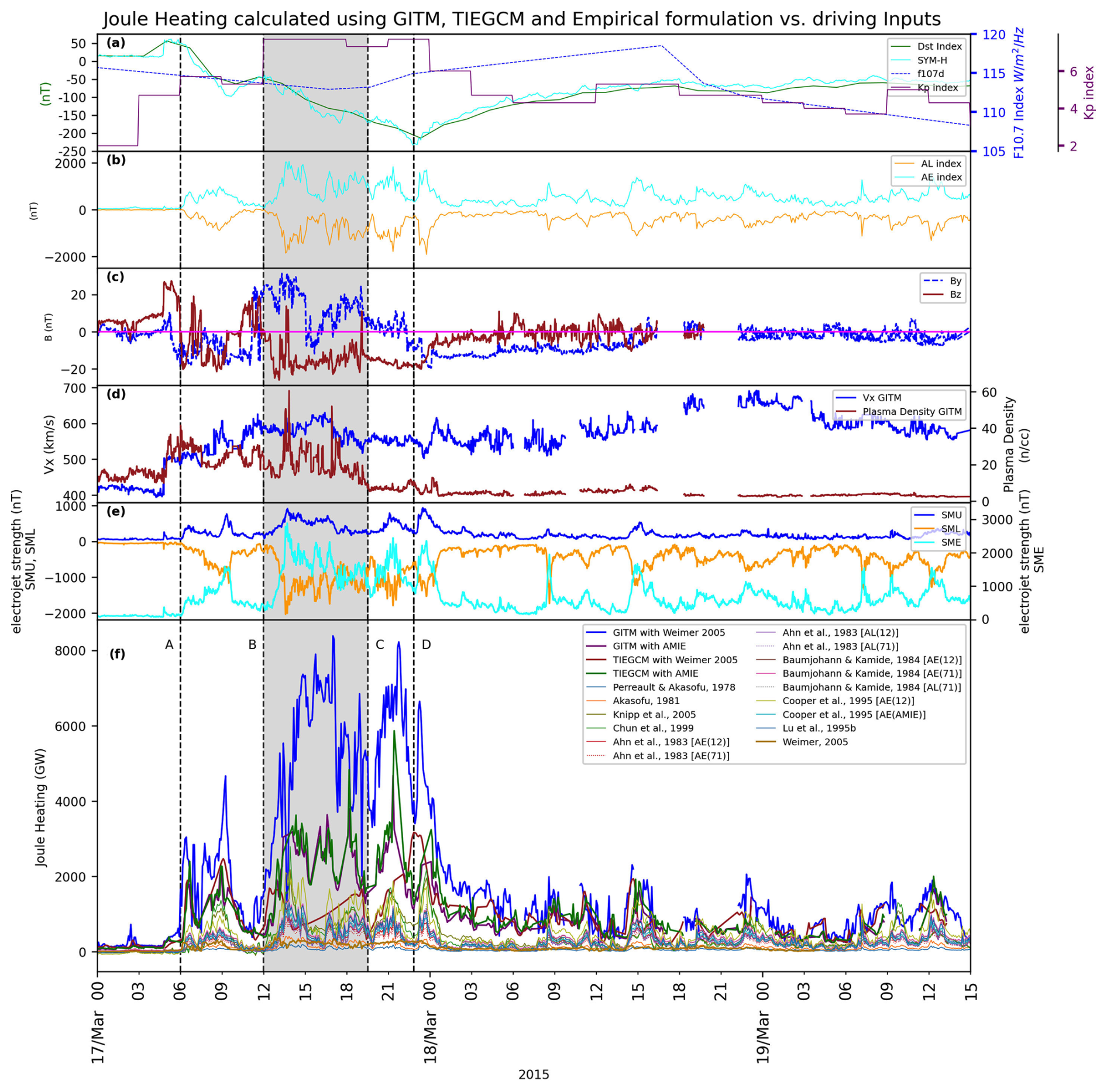
Figure 1 Joule Heating in combination with Geophysical Indices and used quantities. (a) Dst (green), SYM-H (cyan), F10.7 (dashed blue) and Kp (purple) space indices. (b) AL (orange) and AE (cyan). (c) B_y (dashed blue) and B_z (brown) IMF components. (d) V_x (blue) and Plasma Density (brown). (e) SME (cyan), SMU (blue) and SML (orange). (f) Joule Heating from various GCMs and Emprical models as marked. The vertical dashed lines (A, B, C, D) mark specific time steps, as follows: line A marks the first southward turning of B_z; the period between lines B and C mark a period with maximum discrepancies between TIE-GCM_Weimer and GITM_Weimer; and line D marks the time of minimum Dst and SYM-H indices.

3.2 Model Drivers and Inputs

As described above, GITM and TIE-GCM are externally driven by the specification of electric fields and auroral precipitation. In this study the following four different runs are performed and inter-compared:

1. GITM with the Weimer electric field model and the Feature Tracking of Aurora (FTA) Wu et al. (2021) empirical model, hereafter referred to as GITM_Weimer

2. TIE-GCM with the Weimer electric field model and the Emery et al. (2012) empirical auroral model, hereafter referred to as TIE-GCM_Weimer

3. GITM with the AMIE data assimilation model for both the electric fields and auroral inputs, hereafter referred to as GITM_AMIE

4. TIE-GCM with the AMIE data assimilation model for both the electric fields and auroral inputs, hereafter referred to as TIE-GCM_AMIE

Runs 1 and 2 utilize the same electric field specification based on the Weimer model, albeit employing different auroral models. It is noted that these configurations represent the default (and thus more commonly used) setups for the two models, and hence identifying differences in the estimates of Joule heating during active times is of importance. In further detail, with respect to Run 1, GITM uses a two-step process to model auroral inputs: in a first step, the empirical model of Wu et al. (2021) is used to specify the auroral oval latitude, local time maps of the average energy and energy flux; subsequently, taking the average energy, energy flux and mass density of the thermosphere, the ionization rate is calculated as a height profile throughout the thermosphere/ionosphere using the approach described in Sharber et al. (1996). Runs 3 and 4 utilize identical high-latitude drivers, both for the electric field specification and auroral input, and can thus be directly inter-compared. In terms of their initialization, GITM was run for a duration of 24 h prior to the onset of the solar storm. This period allowed for the stabilization of the model in terms of density, wind, and temperature outputs. TIE-GCM was initiated with a history file dated 15 March 2015, marking the start of this simulation.

It is noted in particular that the Weimer 2005 model is the default electric field specification for both GCMs and relies on certain Interplanetary Magnetic Field (IMF) parameters as input, including plasma density, solar wind velocity V_x (in the Sun-Earth direction), and the perpendicular orientation of the solar wind magnetic field B_y and B_z. The AMIE procedure is a data assimilation method which provides maps of high-latitude electric fields, currents, and the associated magnetic variations based on collections of localized observational data. In addition to IMF parameters, both GITM and TIE-GCM use as input the daily F10.7 index, an 81 d average of F10.7 and the 3 hourly Kp index. It is noted that TIE-GCM uses the above inputs with a 15 min resolution, but calls the IMF data every 1 min, whereas GITM uses all the above inputs with a 1 min resolution. Moreover, GITM requires as input the maximum eastward auroral electrojet strength (SMU), the maximum westward auroral electrojet strength (SML) and the difference between the two (SME). SMU, SML, and SME are referred to as SuperMAG indices and are analogous to AU, AL, and AE; they have been introduced as high spatial resolution alternatives to AU, AL, and AE (Gjerloev, 2012; Bergin et al., 2020) and are used herein to drive FTA model.

Panels (a) through (e) of Fig. 1 present the aggregated driving inputs of GITM and TIE-GCM, as described above, as well as the indices used as inputs for the empirical parameterizations of Joule heating, as follows: Panel (a) presents the Dst index (green color), the SYM-H index (dark-cyan color), the 3 hourly Kp index (purple) and the daily F10.7 index (blue dashed line). Panel (b) shows the AL index (orange) and the AE index (cyan). Panel (c) shows the IMF components, B_y (blue) and B_z (brown), in Geocentric Solar Magnetospheric (GSM) coordinates, for the duration of St. Patrick's Day storm; the vertical line marked as A indicates the first southward turning of B_z, indicating the start of the main phase of the storm, while vertical line B in the same figure indicates the start of a prolonged period when B_z remains southward; this is further discussed below. Panel (d) presents the solar wind velocity V_x along the Sun-Earth line (blue solid line) and the plasma density, in units of cm⁻³ (brown solid line). Panel (e) presents the maximum eastward auroral electrojet strength (blue solid line), the maximum westward auroral electrojet strength (blue dashed line) and the difference between the two (brown solid line), which are used in driving the GITM model in addition to the inputs shown in panels (a), (d), and (e).

3.3 Empirical Formulations

Further to the calculation of Joule heating rates in GITM and TIE-GCM, ionospheric dissipation through Joule heating is commonly approximated via empirical formulations that use geomagnetic indices as input. Several studies have derived empirical relationships for the quantification of hemispheric and global Joule heating that are using the AE or AL indices as inputs; these include the studies by Perreault and Akasofu (1978), Akasofu (1981), Ahn et al. (1983), Baumjohann and Kamide (1984), Cooper et al. (1995), Lu et al. (1995). Later on, Chun et al. (1999) estimated Joule heating with a quadratic fit to the Polar Cap (PC) index. Expanding upon the work of Chun et al. (1999), Knipp et al. (2005) proposed an empirical formula based on the PC and the Disturbance Storm Time (Dst) indices. Moreover, Weimer (2005) proposed another method to estimate Joule heating; it is noted that in the study of Weimer (2005) Joule heating and Poynting flux are used interchangeably. A summary of the above studies and the corresponding relationships as well as constraints in terms of season or hemisphere where these are applicable are presented in Table 1.

Perreault and Akasofu (1978)Akasofu (1981)Ahn et al. (1983)Ahn et al. (1983)Ahn et al. (1983)Ahn et al. (1983)Baumjohann and Kamide (1984)Baumjohann and Kamide (1984)Baumjohann and Kamide (1984)Cooper et al. (1995)Cooper et al. (1995)Lu et al. (1995)Chun et al. (1999)Knipp et al. (2005)Weimer (2005)

Table 1 Empirical Formulas for Joule Heating Estimations.

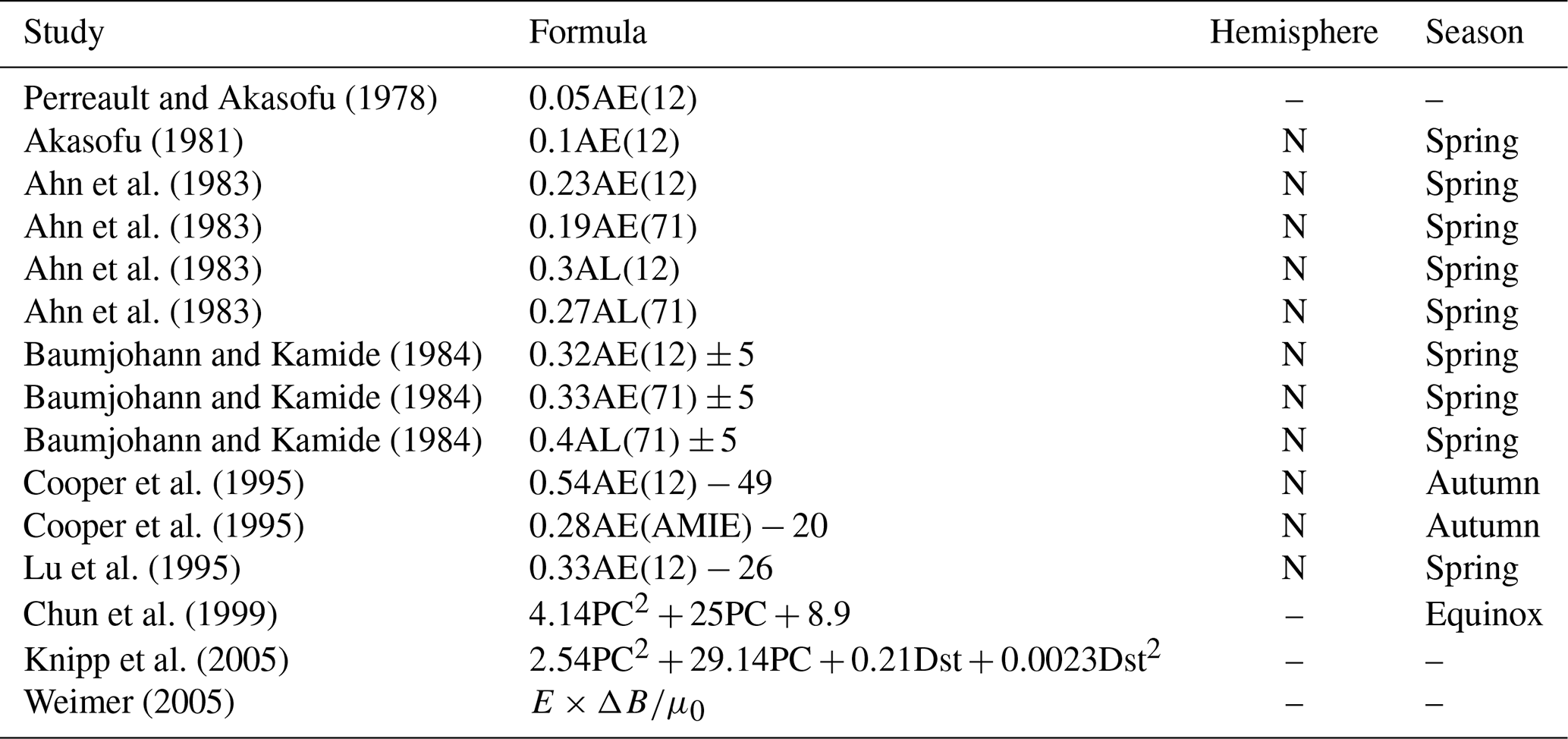
* The numbers in parentheses indicate the number of magnetic stations used in the study.

The AE and AL indices were used in the first twelve empirical formulations of Table 1 with a 1 min resolution, and were obtained from the World Data Center (WDC) for Geomagnetism, Kyoto, Japan. The Polar Cap index, also used with a 1 min resolution, consists of the Polar Cap North (PCN) index and the Polar Cap South (PCS) index. PCN index is taken from the National Space Institute, Technical University of Denmark (DTU, Denmark) and PCS index from the Arctic and Antarctic Research Institute (AARI, Russian Federation). The Dst index was obtained with a 1 h resolution from WDC, Kyoto, Japan. In order to calculate Joule heating according to Knipp et al. (2005) with a 1 min resolution, we replaced the 1 h Dst index with the SYM-H index at 1 min resolution from WDC, Kyoto, Japan; as discussed in Wanliss and Showalter (2006), the Dst and SYM-H indices are considered equivalent but with different time resolutions. A comparison between the two indices is presented in Fig. 1a. The datasets used in this study are readily available at Pirnaris et al. (2024).

3.4 Model Runs

In terms of resolution of the two GCMs, the TIE-GCM run was performed with a spatial resolution of 2.5° in latitude and longitude, 4 grid points per scale height and a time step of 30 s. The GITM run was performed with a resolution of 2° in latitude and 4° in longitude. The altitude resolution of GITM is 3 grid points per scale height and the temporal resolution is 10 s. The resulting output datasets were then converted to a common format for further processing. The datasets and the code are available through Pirnaris et al. (2024). Models Runs were performed on a CPU-based machine with 64GB RAM and an Intel(R) Core(TM) i9-9900K CPU @ 3.60 GHz.

In Fig. 1f the globally-integrated Joule heating rates are presented as calculated using the four GCM runs and the empirical models, as follows: The Joule heating rates as calculated according to the (i) GITM_Weimer, (ii) GITM_AMIE, (iii) TIE-GCM_Weimer, and (iv) TIE-GCM_AMIE runs are marked, respectively, with (i) a thicker dark blue line; (ii) a thicker dark purple line; (iii) a thicker brown line; and (iv) a thicker green line; and Joule heating rates as estimated according to the various empirical formulations of Table 1 are plotted with thinner lines, as marked in the inset of the figure, in chronological order. It is noted that several of the empirical formulations listed in this table give hemispheric estimates of Joule heating. In order to compare against the results presented in Fig. 1, these were multiplied by a factor of 2 to obtain approximations of the global values of Joule heating.

In order to investigate the inter-hemispheric asymmetries of Joule heating, in Fig. 2 the integrated Joule heating is plotted separately over the Northern and Southern Hemispheres, in panels (a) and (b), respectively. The ratio between Joule heating in the Northern Hemisphere over Joule heating in the Southern Hemisphere $(\text{NH}/\text{SH})$ is plotted separately for each of the four GCM runs as follows: in panel (c), $\text{NH}/\text{SH}$ is plotted with solid lines for GITM_Weimer (blue) and TIE-GCM_Weimer (brown); and in panel (d), $\text{NH}/\text{SH}$ is plotted with dashed lines for GITM_AMIE (blue) and TIE-GCM_AMIE (brown).

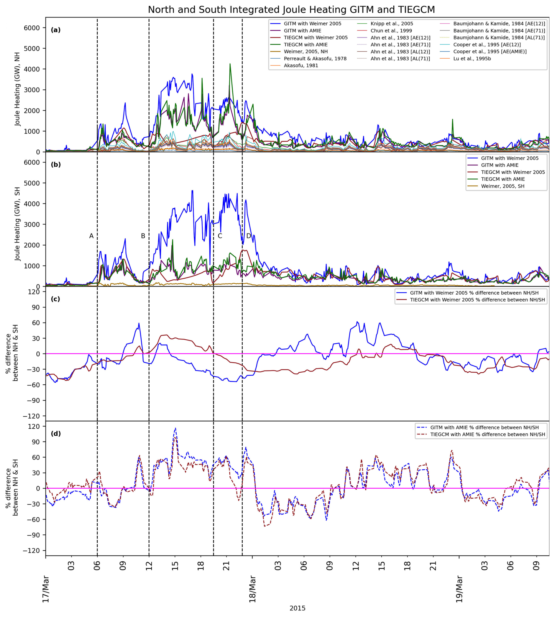
Figure 2 Time-series of the hemisphericaly-integrated Joule Heating in (a) the Northern Hemisphere (NH) and (b) the Southern Hemisphere (SH). (c) Percentage difference between NH & SH of GITM_Weimer (blue solid line) and TIE-GCM_Weimer (brown solid line), and (d) percentage difference between NH & SH of GITM_AMIE (blue dashed line) and TIE-GCM_AMIE (brown dashed line).

In order to cross-compare the total amount of Joule heating that is deposited onto each thermospheric hemisphere during St. Patrick's Day storm 2015 as estimated by the two GCMs and the various empirical models, in Fig. 3 the cumulative, time-integrated Joule heating is plotted as a function of time. The corresponding models are color-coded and are listed in the right-hand side of the figure in order of descending Joule heating. The estimated cumulative Joule heating in the northern (southern) hemisphere are plotted in GITM and TIE-GCM with thicker solid (dashed) lines. The thinner lines indicate Joule heating estimates over the Northern Hemisphere according to the empirical models of Table 1, as marked in the figure's inset. In the cases that empirical estimates are based on indices obtained from 12 ground stations, the results are plotted with a thin solid line, whereas estimates that are based on 71 stations are plotted with a thin dotted line.

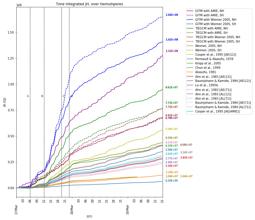
Figure 3 Time-integrated (cumulative) global Joule heating according to GITM and TIE-GCM driven by the Weimer and AMIE high latitude electric field specifications and various empirical models, as marked, listed from highest to lowest Joule heating values.

In Fig. 4 three snapshots of the height-integrated Joule heating are shown as polar plots over the Northern Hemisphere, based on GITM_Weimer (panel a) and TIE-GCM_Weimer (panel b) simulations. Three characteristic times during St. Patrick's Day storm on 17 March 2015 are plotted: 06:20 UT (left-hand side panels), marked as line A in Figs. 1–3, corresponding to the beginning of the storm; 14:10 UT (middle panels), corresponding to the time of maximum percentage difference in Joule heating between GITM_Weimer and TIE-GCM_Weimer (not marked with a line in the above figures); and 22:50 UT (right-hand side panels), marked as line D in the above figures, which corresponds to the peak of the storm, as indicated by the minimum in Dst. In Fig. 4c and d, the height-integrated Joule heating is plotted for the same time-steps as those presented in panels (a) and (b), but based on GITM_AMIE (panel c) and TIE-GCM_AMIE (panel d). The comparisons between Fig. 4a and b at the top and panels (c) and (d) show that, apart for the large differences in the amplitudes of Joule heating between GITM and TIE-GCM, the distribution of Joule heating in longitude and latitude shows notable similarities, except for the middle plots of (a) and (b), which represent calculation using the Weimer model, with slight variations in the localization and extent of the spatial structures where Joule heating appears.

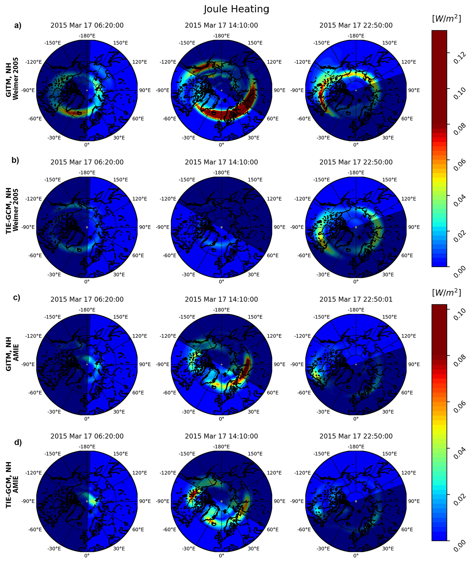
Figure 4 Height-integrated Joule Heating as calculated over the Northern Hemisphere for three different snapshots during St. Patrick's Day event, as marked. (a) GITM_Weimer, (b) TIE-GCM_Weimer, (c) GITM_AMIE, (d) TIE-GCM_AMIE.

4 Discussion

Based on the simulation results shown in Figs. 1 and 2, a significant disagreement is observed in the values of the globally-integrated Joule heating rates as obtained through TIE-GCM and GITM during the storm main phase, and in particular between 17 March, 06:00 UT, which marks the first southward turning of B_z and is noted with line A in the above figures, and 17 March, 22:50 UT, which is the time of minimum Dst, and is marked with line D. This disagreement is noted both in terms of amplitude as well as in terms of the overall shape and evolution of Joule heating, and is more prominent when the Weimer 2005 model is used for the specification of the high-latitude electric field model. A better agreement between the two GCMs is found when the AMIE model is used, even though at times there are significant differences, such as around 17 March, 22:00 UT. As detailed in Sect. 2.3, the two GCMs use similar formulations for the calculation of Joule heating; also the electric field and the particle precipitation models are the same. Thus, a possible reason for these differences is related to the different spatial resolutions that are employed in the two models. Another possible reason is the different way that the two models treat vertical momentum and eddy diffusion: As discussed in Sect. 2.1, in GITM the complete vertical momentum equation is solved (see, e.g. Ullrich et al., 2010), which could lead to significant differences, in particular in the lower regions of the model, where also the eddy diffusion is expected to be larger. A more detailed parametric study could shed more light onto the causes of these discrepancies. A general order-of-magnitude agreement is observed in the first part of the storm, from 17 March, 00:00–12:00 UT, as well as after the time of minimum Dst and in the recovery phase of the storm.

Further to the models that have been used in this study, Suji and Prince (2018) used the OpenGGCM (Raeder et al., 2001) to calculate the global ionospheric Joule heating during St. Patrick's Day 2015 geomagnetic storm. The values of global Joule heating rates that are presented in Fig. 7 of Raeder et al. (2001) are considerably higher than the values reported herein. Such disagreements in the comparisons of simulated Joule heating have been discussed extensively by, e.g. Cosgrove and Codrescu (2009), who investigated the underestimation of Joule heating caused by high-latitude electric field variability in electric field models and addressed the notion of “electric field variability” as a potential source of this underestimation. Similarly, Lu et al. (2023) used TIE-GCM driven with AMIE to gain insights into the 2015 St. Patrick's Day storm's impact on the ionosphere-thermosphere (IT) system by utilizing observations of high-latitude forcings, specifically aurora and electric fields, along with the TIE-GCM. Verkhoglyadova et al. (2017), utilized GITM along with empirical models and proxies derived from in situ measurements to estimate the energy distribution within the IT system during the solar storms events of 16–19 March of 2013 and 2015, while Zhu and Ridley (2016), calculated Joule heating rates through GITM simulations and revealed that the globally averaged thermospheric temperature (T_n) was underestimated under quiet geomagnetic conditions.

It is noted that the comparative analyses presented above in Figs. 1–4, and also the analyses in the works by, e.g. Suji and Prince (2018), Raeder et al. (2001), Lu et al. (2023), Verkhoglyadova et al. (2017), Zhu and Ridley (2016) and other similar studies can not, on their own, bring closure as to which model provides the most accurate estimates of storm-time Joule heating. Instead, the analyses herein can provide the range of variability of Joule heating according to the different models and drivers, from which the uncertainty in estimating and predicting the state of the LTI can be approximated. Furthermore, the large discrepancies that are demonstrated by these model runs indicate that the exact quantification of Joule heating is a critically missing parameter in the LTI energetics. This is due to the lack of direct, comprehensive measurements in this region of the Earth geospace environment, as the altitude range where Joule heating maximizes is too high to be sampled with probes on aerial vehicles and balloons and too low for typical spacecraft, making direct measurements therein challenging (see, e.g. Sarris, 2019; Palmroth et al., 2021). Thus, the results of this study reinforce the current motion in the scientific community that efforts must be taken to close this gap, by dedicated missions that can provide all missing parameters required to estimate Joule heating, as outlined in Eqs. (6), (8), and (15). Such mission concepts have been proposed and are being actively investigated (see, e.g. Sarris et al., 2020; Pfaff et al., 2022; ESA/NASA-ENLoTIS-Report, 2024).

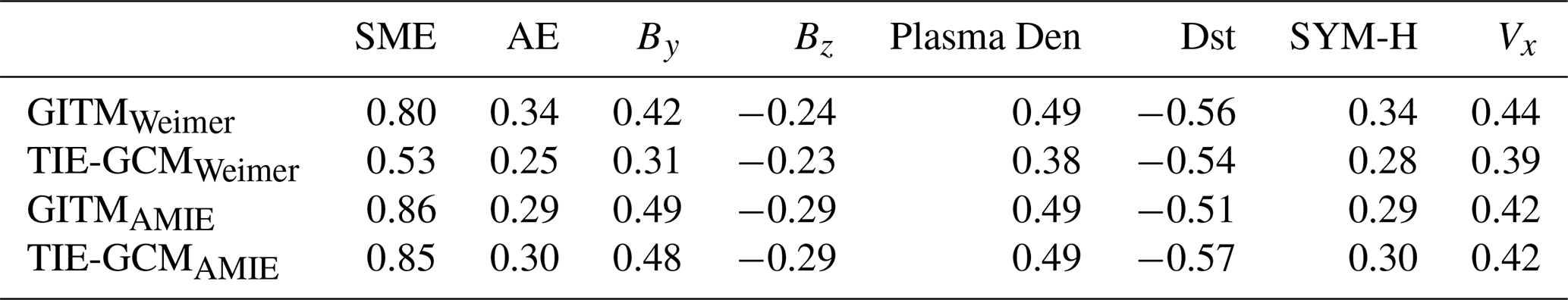
In order to identify the key driving parameters for the discrepancies in Joule heating between the different model runs, a Spearman's Rank Correlation analysis (Spearman, 1904) has been performed between the four Joule heating rate time series and each of the input parameter time series that are shown in panels (a) through (e) of Fig. 1. The results are shown comprehensively in Table 2. Through this correlation analysis, it is found that Joule heating is strongly related to the SME electrojet strength in both the GITM_AMIE, TIE-GCM_AMIE, and GITM_Weimer, with correlation coefficients of 0.86, 0.85, and 0.80 respectively; in TIE-GCM_Weimer, this correlation drops to 0.53. The correlation coefficients of the four runs with B_y are similar, but slightly smaller in TIE-GCM_Weimer, whereas the correlation coefficients of the four runs with B_z are similar but negative, indicating anti-correlations, with, again, a smaller correlation (in absolute value) in TIE-GCM_Weimer. The anti-correlation between Joule heating and B_z is attributed to the enhanced Joule heating during southward turnings of the IMF; the dependence of Joule heating on B_z has been examined in more detail in various studies, such as, e.g. by McHarg et al. (2005). The correlation with solar wind plasma density is lower for TIE-GCM_Weimer and similar between the other three runs. The correlation with the absolute value of Dst is similar among all four model runs, and is the second most significant correlation, after SME. Finally, the correlation with SYM-H is similar for all four model runs, and is comparable to the correlation with AE and B_z.

Table 2 Correlation coefficients between the GITM_Weimer, TIE-GCM_Weimer, GITM_AMIE and TIE-GCM_AMIE runs and their main input parameters.

In Figs. 1 and 2 a notable difference can be seen in Joule heating when it is calculated in TIE-GCM_Weimer compared to GITM_Weimer. This is particularly evident in the period from ∼12:00UT to ∼19:30UT on 17 March 2015, which is shown in the gray-shaded region that is bounded by lines B and C. During this time, it can be seen that GITM_Weimer is well correlated with the SME electrojet strength, with an increase and subsequent decrease in SME being accompanied by a corresponding increase followed by a gradual decrease in Joule heating, whereas, in contrast, Joule heating in TIE-GCM_Weimer shows an initial drop followed by a gradual increase. This increase appears to be correlated with the prolonged southward turning of IMF B_z during this time, which does not appear to affect in the same way the calculations of Joule heating in GITM_Weimer. Furthermore, Joule heating as computed by GITM_Weimer exhibits a higher magnitude compared to the results from TIE-GCM_Weimer, as well as the results from GITM_AMIE and TIE-GCM_AMIE. This is attributed to the differences in the auroral precipitation model that is used for the two runs that utilize the Weimer 2005 model as input, GITM_Weimer and TIE-GCM_Weimer, as is also indicated by the differences in the HP power presented in Fig. 1f. As discussed above, the GITM_Weimer run uses the FTA model Wu et al. (2021), while TIE-GCM_Weimer run uses the analytical auroral model of Roble and Ridley (1987) and Emery et al. (2012). On the other hand, GITM_AMIE and TIE-GCM_AMIE use the same auroral precipitation model, described in Richmond and Kamide (1988), and show better agreement in terms of shape and magnitude, as shown in Fig. 1f, especially between lines B and C. These results highlight the significance of particle precipitation in the overall electrodynamic coupling within the LTI (e.g. Palmroth et al., 2021), since precipitation leads to increased ionospheric conductivity (Aksnes et al., 2004), which is an essential contributor to Joule heating. A further parametric study based on model runs under different parameterizations of particle precipitation would enable a thorough evaluation on the inter-relationship between particle precipitation, conductivity and Joule heating, and a quantitative assessment of the extent to which the differences in the model run results are indeed correlated to differences in particle precipitation and conductivity. It is also noted that in the TIE-GCM_Weimer run a much lower variability is observed in Joule heating compared to the other three runs, which have a larger peak-to-peak fluctuation in the amplitudes of Joule heating. It is speculated that this is due to the lower level of correlation between the TIE-GCM_Weimer and the SME index, compared to the other three runs, as discussed above and as shown in Table 2. Finally, it is noted that all empirical formulations tend to underestimate the overall Joule heating when compared to all four GCM runs, as shown in Fig. 1f. A possible reason is that empirical models in general rely on historical data and statistical models that may not adequately capture the complex, non-linear dynamics and feedbacks that drive extreme events, such as solar storms. GCMs on the other hand, while still having limitations, attempt to simulate these complex processes, potentially offering a more realistic representation of extreme events.

Comparing the time series of the hemispherically-integrated Joule heating from the two GCMs with the corresponding values from the empirical models, as is plotted in Fig. 2a, it can be seen that there is a closer agreement between the empirical models and TIE-GCM_Weimer rather than with GITM_Weimer. Furthermore, comparing the percentage differences between the hemispherically-integrated Joule heating in the northern and Southern Hemispheres as calculated with GITM_Weimer and TIE-GCM_Weimer, which are plotted in Fig. 2c, it can be seen that the two model runs show significantly different inter-hemispheric asymmetries, especially during times of enhanced Joule heating, between lines B and D. During this time, GITM_Weimer calculations show higher Joule heating in the Southern Hemisphere by up to ∼55 %, while TIE-GCM_Weimer shows initially higher Joule heating in the Northern Hemisphere by up to ∼35 % and subsequently higher Joule heating in the Southern Hemisphere by up to ∼40 %, with a time-lag of approximately 5 h. The percentage differences between the hemispherically-integrated Joule heating from GITM_AMIE and TIE-GCM_AMIE are presented in Fig. 2d and show almost the same inter-hemispheric asymmetry during the simulation period. Both GITM_AMIE and TIE-GCM_AMIE show higher Joule heating in the Northern Hemisphere by up to ∼116 % and ∼100 % respectively during the storm main phase, while during the recovery face of the storm Joule heating deposition in the Southern Hemisphere becomes higher by up to ∼60 % for the GITM_AMIE and up to ∼74 % for the TIE-GCM_AMIE.

By comparing the time-integrated (cumulative) hemispherically-integrated Joule heating, as shown in Fig. 3, it can be seen that, whereas higher Joule heating is observed in the Southern Hemisphere (SH; dashed lines) than the Northern Hemisphere (NH; solid lines) for the GITM_Weimer (blue) and TIE-GCM_Weimer (brown) simulations, the opposite is observed in the case of GITM_AMIE (purple) and TIE-GCM_AMIE (green), with the Northern Hemisphere receiving larger amounts of heating over the course of the storm.

Such asymmetries in the hemispherically-integrated Joule heating have been identified by several studies, and have been associated with the Earth's asymmetric magnetic field configuration: as discussed in, e.g. Laundal et al. (2017) and references therein, the dipole tilt and eccentricity shift in the Earth's magnetic field leads to a displacement between the geographic and geomagnetic poles, which is larger in the Southern Hemisphere, and to a difference in the magnetic field strength between north-south conjugated latitudes. Hong et al. (2021) used GITM to study the impacts of different causes on the inter-hemispheric asymmetry of the ionosphere-thermosphere system, including inter-hemispheric differences associated with the solar irradiance, the geomagnetic field, and the magnetospheric forcing under moderate geomagnetic conditions. Hong et al. (2021) derived an index of inter-hemispheric asymmetry for Joule heating, which, for solar equinox conditions, was found to be as large as ∼43 % due to the asymmetric geomagnetic field, ∼28 % due to asymmetric particle precipitation and ∼35 % due to asymmetric ion convection pattern. Pakhotin et al. (2021), using Swarm satellite observations, demonstrated that the Northern Hemisphere generally receives a higher electromagnetic energy input across all seasons. This preference has also been observed using DMSP satellites (Knipp et al., 2021). Cosgrove et al. (2022) also investigated the appearance of such asymmetries, and revealed a considerable asymmetry in the hemispherically integrated Poynting flux between the Northern Hemisphere (NH), which generally showed higher flux, and the Southern Hemisphere (SH). More recently, Smith et al. (2023), also investigated inter-hemispheric asymmetries, looking into the role of solar wind driving conditions and the accuracy of Joule heating estimates using GITM (Weimer and AMIE) runs during the 2013 St. Patrick's Day geomagnetic storm (note the different year compared to the 2015 St. Patrick's Day geomagnetic storm that was simulated herein). They showed that AMIE driven simulations lead to stronger inter-hemispheric asymmetries in Joule heating compared to Weimer 2005 driven runs, and found higher Joule heating deposition in the Southern Hemisphere for the first phase of the 2013 St. Patrick's Day geomagnetic storm for both Weimer and AMIE simulation, which reversed in later phases of that storm.

The results presented herein indicate that the appearance of inter-hemispheric asymmetries are largely dependent on the external drivers that are used (primarily the electric field and auroral precipitation specifications). The results show that both the GITM_AMIE and TIE-GCM_AMIE runs have almost the same inter-hemispheric asymmetry and Joule heating magnitude, as observed in Fig. 2d, denoting that the implementation of the two GCMs delivers almost the same results under the same driving conditions (electric field and auroral precipitation). This is not confirmed in the case of the GITM_WEIMER and TIE-GCM_WEIMER runs in their default configuration, as observed in Fig. 2c, where the Joule heating deposition is largely variable, as discussed above. Taking into account that both of these runs use the Weimer 2005 model as a high latitude electric field driver, these results show that Joule heating is highly dependent on the auroral precipitation model.

It is noted that, as discussed above, both GITM and TIE-GCM use the International Geomagnetic Reference Field (IGRF) magnetic field model, and hence the asymmetries in the magnetic field are the same; thus the differences in the observed behavior are more likely attributed to the asymmetric particle precipitation and the asymmetric ion convection pattern. However the exact causes of the different behavior of TIE-GCM and GITM when run using different external drivers with respect to the inter-hemispheric differences is a subject that requires further research through parametric studies.

5 Summary and conclusions

Based on GITM and TIE-GCM driven by the Weimer 2005 and AMIE models, as well as on various empirical formulations, globally- and hemispherically-integrated Joule heating rates were calculated during St. Patrick's Day storm of 2015. It is found that Joule heating rate estimates in the global circulation models, GITM and TIE-GCM, for all external drivers, are generally higher in magnitude than any of the empirical models. Comparing GITM_AMIE and TIE-GCM_AMIE, it is found that they are in better agreement compared to GITM_Weimer and TIE-GCM_Weimer in terms of amplitudes, peak-to-peak variability and inter-hemispheric asymmetry. In comparing the latter two models, it is found that Joule heating derived using TIE-GCM_Weimer has lower amplitudes and also a lower peak-to-peak variability than GITM_Weimer. Significant variations that are observed are most likely attributed to the different precipitation models that are employed. This comparison is essential, as it reflects the default parameterizations of the two GCMs. On the other hand, Joule heating results derived using TIE-GCM and GITM driven with AMIE data can be directly compared. Through a correlation analysis, and also by comparing the heating rates for a period of clear anti-correlation in the heating rate trend between the two models, it is found that both the TIE-GCM_AMIE and GITM_AMIE runs are strongly driven by the SME index; this is not the case for the two Weimer runs, where GITM_Weimer is strongly driven by the SME index, which is not present in TIE-GCM_Weimer. It is also found that Joule heating in TIE-GCM_Weimer is affected by the southward turnings of B_z to a larger extent than GITM_Weimer. Joule heating calculated by the two GCMs using AMIE inputs shows similar values and peak-to-peak variability, compared to Joule heating derived using GCMs Weimer runs.

By integrating the Joule heating estimates separately in each hemisphere, it is found that GITM_Weimer shows a larger degree of asymmetry during the main phase of the storm than TIE-GCM_Weimer. Furthermore, by integrating Joule heating in time it is found that the cumulative Joule heating input to the thermosphere is larger as calculated in GITM_Weimer in the SH and NH, followed by the various GCM runs, and then by the various empirical models. A factor of 2 difference is observed between the largest and smallest cumulative Joule heating when comparing different GCM runs, whereas a factor of 25 is observed between the largest and smallest cumulative Joule heating, when all models (GCMs and empirical) are inter-compared. The localization (latitudinal and longitudinal distribution) of Joule heating in the two models exhibits slight variations, as depicted in characteristic time steps, as presented in Fig. 4.

In conclusion, as also demonstrated by the discrepancies in the above cross-comparisons between physics-based and empirical models, Joule heating remains to this date a quantity with many discrepancies in its estimation, showing large gaps in its understanding and parameterization. At the same time, it is a quantity of great significance in LTI processes, as it determines to a great extent the overall energy budget, in particular during active solar and geomagnetic conditions. Thus, characterizing its magnitude, time evolution and variability within the latitude and altitude region where it maximizes and accurately parameterizing Joule heating by solar and geomagnetic conditions are critical missing pieces in accurately understanding and modeling LTI processes. This demonstrates the currently limited knowledge about Joule heating and emphasizes the need for comprehensive measurements, such as outlined in Sarris et al. (2023a), to accurately quantify Joule heating.