Modeling magnetopause location for 4D drift-resolved radiation belt codes: Salammbô model implementation

We present a new semi-analytical magnetopause location model specifically designed for 4D drift-resolved radiation belt modeling codes. We specifically designed this magnetopause location model for the 4D version of Salammbô, but it can be adaptable to similar codes. The model combines parameterization by the Kp index with a representation of the magnetopause in L^∗ geomagnetic coordinates and magnetic local time (MLT). It is based on a 20-year dataset relying on computed magnetopause stand-off distances using a solar wind database and a relevant magnetopause model, then converted into L^∗ geomagnetic coordinates for all dayside MLT. Through the statistical analysis of this dataset, the model was formulated and validated against a magnetopause crossing catalog. Its performance was benchmarked against the magnetopause location model previously developed for the 3D version of the Salammbô code. The results demonstrate an improvement in predicting the magnetopause position in L^∗ across dayside MLT sectors, with enhanced accuracy in the dawn sector. These results highlight the model's ability to model the magnetopause location in L^∗ across dayside MLT sectors. This advancement may be specifically useful for simulating magnetopause shadowing in ring current and radiation belt modeling codes.

1 Introduction

The magnetopause, the outer boundary of Earth's magnetosphere, represents the interface between the magnetospheric magnetic field and the hot tenuous plasma of the solar wind. First theorized by Chapman and Ferraro (1933), this boundary delimits a protective cavity around Earth. It shields various internal structures, such as the Van Allen radiation belts, from the solar wind. These belts are composed of charged particles confined by Earth's magnetic field. They are highly dynamic structures, responding strongly to enhanced geomagnetic activity. The magnetopause, as the boundary of the magnetosphere, plays a critical role in influencing the behavior of the radiation belts. Accurate characterization of the magnetopause is essential for understanding and modeling this dynamic.

Modeling of Earth's radiation belts has largely been based on physical codes (Beutier and Boscher, 1995; Bourdarie et al., 1996; Glauert et al., 2014b; Reeves et al., 2008; Subbotin and Shprits, 2009). Among them, ONERA's Salammbô code is a well-established physical code with versions for both electrons and protons (Beutier and Boscher, 1995; Bourdarie et al., 1996). However, challenges remain, particularly for accurately modeling particle loss processes through wave–particle interactions and dropouts. This paper specifically examines how magnetopause modeling may be implemented to help reproduce the rapid and intense particle losses best during specific dropouts, namely the magnetopause shadowing effect, which impacts a broad energy range of protons and electrons across various drift shells.

A characterization of dropouts was first conducted by Bailey (1968), who described it as an increased electron precipitation on the dayside during a geomagnetic storm. Although the process is not fully understood, the literature agrees on dropouts being related to two major mechanisms. The first involves particle precipitation into the atmosphere due to wave–particle interactions, through either chorus waves (Morley et al., 2010) or EMIC waves (Xiang et al., 2017). The second mechanism is the magnetopause shadowing effect. This process happens when the magnetopause moves inward due to compression during geomagnetic storms. At the same time, magnetospheric ultra-low-frequency (ULF) waves cause outward radial diffusion, pushing particles away from Earth toward the dayside magnetosphere (Degeling et al., 2013).

Several models have been developed for analytically modeling the location of the magnetopause (Fairfield, 1971; Formisano et al., 1979; Holzer and Slavin, 1978; Petrinec and Russell, 1991; Petrinec and Russell, 1996; Roelof and Sibeck, 1993; Shue et al., 1997, 1998; Sibeck et al., 1991). The majority of these models use an elliptical or parabolic function to represent the magnetopause. The magnetopause model by Shue et al. (1997, 1998), referred to in the following as the Shue model, is widely adopted for its accuracy (Shue et al., 2000) and ease of implementation. It is an analytical model that is built on a database of more than 500 magnetopause crossings observed by the ISEE 1 and 2 (Durney and Ogilvie, 1979), AMPTE/IRM (Bryant et al., 1985), and IMP 8 satellite missions. This model has also been used as a foundation for further improved models. Notably, Lin et al. (2010) developed an extended version of the Shue model that incorporates an asymmetric high-latitude magnetopause. It was also used to study the impact of magnetopause shadowing on electron radiation belt dynamics. Matsumura et al. (2011) investigated the correlation between magnetopause shadowing and outer electron radiation belt losses during geomagnetic storms using this model. The observed strong correlation proved that magnetopause shadowing is crucial for modeling the dynamics of radiation belts. Consequently, several magnetopause shadowing models have been developed for radiation belt modeling codes (Glauert et al., 2014a; Herrera et al., 2016; Wang et al., 2020). These are detailed in the next section.

The particles in the radiation belts are confined by Earth's magnetic field that shapes their behavior. To accurately represent the motion of charged and trapped particles around Earth, all existing codes rely on geomagnetic coordinates rather than geographic coordinates. One of the key geomagnetic coordinates is L^∗, also referred to as the Roederer parameter (Roederer, 1967; Roederer and Zhang, 2014). The accurate modeling of the magnetopause shadowing phenomenon for radiation belt modeling codes relies on the magnetopause location given in the relevant adiabatic coordinates system. Herrera et al. (2016) characterized the magnetopause shadowing effect during geomagnetic storms for the Salammbô code as a function of Kp and expressed in terms of L^∗. However, this research focused exclusively on the drift-averaged version of the Salammbô code (also called Salammbô 3D) (Beutier and Boscher, 1995; Varotsou et al., 2005; Bourdarie and Maget, 2012; Dahmen et al., 2024). Yet, Salammbô exists in a drift-resolved version called Salammbô 4D (Bourdarie et al., 1996). The latter considers the magnetic local time (MLT) dimension in order to model the transport of low-energy electrons induced by magnetospheric convective electric fields. Integrating the physical processes represented in Salammbô 3D into the 4D code (including the addition of an MLT dependency) is a complex task. This challenge becomes even more pronounced when addressing the magnetopause shadowing effect, which requires precise knowledge of the magnetopause location. In this study, we propose a simplified magnetopause location model designed to describe the magnetopause position in terms of MLT and L^∗ for 4D radiation belt modeling codes. This model is detailed in Sect. 2. Then we propose a validation of the new magnetopause location model against magnetopause crossing data in Sect. 3, and we summarize our study in Sect. 4.

2 Methodology and model development: from long-term sampled dataset construction to performance assessment

2.1 Theoretical framework of the study

Modeling Earth's radiation belt relies on the resolution of the Fokker–Planck diffusion equation (Schulz and Lanzerotti, 1974). All physical radiation belt modeling code solves this equation using adiabatic invariants such as the L^∗ parameter, which simplifies the equation. Regardless of the level of refinement (1D, 2D, 3D, or 4D), the definition of the magnetopause in L^∗ is essential for radiation belt modeling applications. However, higher levels of refinement lead to increased computational costs.

The Salammbô code addresses this by using an L^∗ grid with different grid sizes to balance accuracy and computational cost. The full L^∗ grid consists of 133 points ranging from 1 to 8, while the smaller grid contains one-fourth of the points. In Salammbô 4D, which includes a supplementary coordinate, MLT, the reduced grid is the preferred option to ensure efficiency. Figure 1 illustrates the spacing between two consecutive grid points (ΔL^∗) as a function of L^∗ for both the full L^∗ grid (blue) and the reduced grid (red). The choice of grid affects the accuracy of the model, with ΔL^∗ variations reflecting the intrinsic uncertainties of grid refinement in Salammbô codes. Consequently, when incorporating a magnetopause model into the Salammbô framework, it is essential that the magnetopause location model does not introduce uncertainties exceeding those inherent to the code.

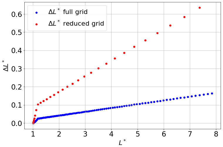
Figure 1 Spacing between two consecutive grid points (ΔL^∗) for the full L^∗ grid (blue) and the reduced L^∗ grid resolution (red) as a function of L^∗.

Expressing the magnetopause location with the geomagnetic parameters L^∗ and MLT is crucial to ensure its adaption to radiation belt modeling codes, and several examples in the literature align with this approach. For example, Glauert et al. (2014a) incorporated the Shue magnetopause model, which provides the magnetopause distance in R_E, into the BAS code (Glauert et al., 2014b) to compute the last closed drift shell, $L_{\mathrm{LCDS}}^{\ast }$, in L^∗. Similarly, the VERB 3D code (Subbotin and Shprits, 2009) also incorporates an $L_{\mathrm{LCDS}}^{\ast }$ calculation to consider the magnetopause shadowing effect in the modeling (Wang et al., 2020). Xiang et al. (2017) and Olifer et al. (2018) demonstrated that using an $L_{\mathrm{LCDS}}^{\ast }$ calculation was more effective in capturing the magnetopause shadowing phenomena than using the distance given in R_E provided by the Shue model. Complementary to these approaches, Herrera et al. (2016) proposed a quantitative estimation of the magnetopause location in L^∗ for the Salammbô 3D code. Their method computes the magnetopause stand-off distance in Earth radii (R_e) using a magnetopause model, from which the corresponding L^∗ value of the magnetopause ($L_{\mathrm{mp}}^{\ast }$) is derived.

In 4D radiation belt modeling, the approach is more complex. The drift motion of particles is no longer integrated out, the modeled energy range extends to lower limits, and a transport term is added to the Fokker–Planck equation. Incorporating particle transport into radiation belt modeling means that the magnetic field is not the sole driver of particle dynamics. The magnetospheric electric fields also play a significant role in influencing particle behavior, as they can modify the particle drift shells significantly. Therefore, directly applying the 3D model of Herrera et al. (2016) to the Salammbô 4D code is not a reasonable strategy. Indeed, a magnetopause location model that integrates both L^∗ and MLT is needed, ensuring its compatibility with 4D radiation belt simulations, while ensuring fast computation and accuracy.

Defining the magnetopause location in terms of MLT and L^∗ presents inherent challenges. In fact, one L^∗ value describes an entire particle magnetic drift shell, making it an integrated parameter over all MLT values. In 4D radiation belt modeling, low-energy particles orbit Earth over relatively long time periods compared to the inward movement of the magnetopause during periods of high geomagnetic activity (Olifer et al., 2018). Therefore, the evolution of these particles' dynamics must account for MLT, and their behavior will be influenced by the magnetospheric electric fields. As the magnetopause moves inward and intersects a drift shell, the fate of trapped particles depends on their location relative to the magnetopause boundary. Particles situated along the portion of the drift shell outside the magnetopause are lost from the system, while those on the inside remain trapped within the radiation belts. However, these particles no longer have a well-defined magnetic drift shell. Instead, their motion is likely to approximate a “virtual drift shell”, guided by the combined influence of Earth's magnetic field and the magnetospheric electric fields (Burger et al., 1985; Stern, 1977).

2.2 Constructing the long-term sampled dataset: from Earth radii to L^∗

The Shue model is axisymmetric around the Sun–Earth line and provides the stand-off distance of the magnetopause in R_E for each MLT value. It is driven by the z component of the magnetic field (B_z) and the solar wind dynamic pressure (D_p), providing a link between the magnetopause location and the upstream conditions in the solar wind (Shue et al., 1998). To express the magnetopause location in terms of L^∗ and MLT, the stand-off distance must be transformed into an $L_{\mathrm{mp}}^{\ast }$. This transformation requires the use of a realistic magnetic field model. Many modern magnetic field models include a magnetopause boundary based on the Shue model (Tsyganenko 2002a, b; Tsyganenko and Sitnov, 2007). In contrast, the Tsyganenko (1989a, b, c) magnetic field model (referred to as T89C) is driven only by the Kp index. While it differs from the other models by not having a built-in magnetopause boundary, its sole dependence on Kp provides an adequate compromise between accuracy and the fast computation of L^∗ values, when compared to more sophisticated ones. Besides, its accuracy has been proven compared to in situ measurements, even during disturbed time and large L^∗ values (Loridan et al., 2019).

The conversion from stand-off distances to $L_{\mathrm{mp}}^{\ast }$ comes anyway with a significant computational cost. The direct calculation of these distances within a radiation belt modeling code would considerably increase the computational time, making it impractical. To address this, we developed a long-term dataset of $L_{\mathrm{mp}}^{\ast }$ values based on the Shue magnetopause model, covering a 20-year period. This dataset allows us to then quantify relationships between L^∗, MLT, and dynamic parameters, reducing the need for in-code calculations.

The dataset construction process is summarized in Fig. 2. It begins with the OMNI database (https://omniweb.gsfc.nasa.gov/, last access: 25 June 2025) (represented in green), which provides measurements of solar wind dynamic pressure (D_p) and interplanetary magnetic field (B_z) values from 2000 to 2020. These values are then used to compute stand-off distances for each hourly MLT bin using the Shue model (depicted in yellow). The conversion of the stand-off distances into $L_{\mathrm{mp}}^{\ast }$ is achieved using the Kp index and the IRBEM library (O'Brien and Bourdarie, 2012) within the Python package SpacePy (Morley et al., 2022). The conversion from R_E to $L_{\mathrm{mp}}^{\ast }$ is performed for each hourly resolved epoch at the magnetic equator. The resulting dataset (shown in blue) contains the corresponding values of Kp, D_p, B_z, and $L_{\mathrm{mp}}^{\ast }$ at every dayside MLT (06:00 to 18:00 MLT).

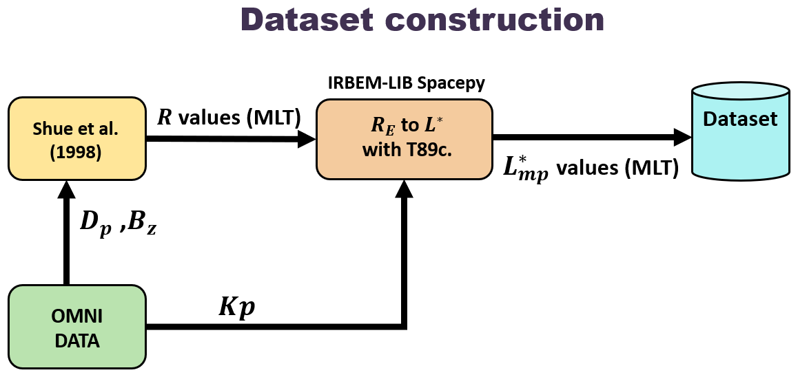
Figure 2 Diagram describing the long-term dataset construction process, using the OMNI data (green) to compute the magnetopause stand-off distance (yellow) and the R_E-to-L^∗ transformation (orange) to build the constructed long-term dataset (blue).

2.3 A semi-analytical magnetopause location model for 4D radiation belt modeling

Building a simple magnetopause model presents significant challenges, as an initial correlation analysis found no clear correlation between D_p, B_z, and Kp. While other studies suggest that Kp is related to D_p and a modified B_z (Andonov et al., 2004), this adds complexity to the model development. Solar wind parameters have only been consistently available since 1995; the Kp index, available since 1932, provides a reliable and long-baseline measure. Since it is the primary driver of both the T89C magnetic field model and the Salammbô code, using Kp for our magnetopause model is advantageous, making it easier to integrate than solar wind parameters.

We conducted a statistical analysis on the computed 20-year dataset to investigate its dependency on the Kp index. The dataset was therefore binned over four Kp ranges (0–2, 2–4, 4–6, 6–9). Figure 3 illustrates the distribution of time-averaged $L_{\mathrm{mp}}^{\ast }$ values across these Kp ranges for MLT sectors between 06:00 and 18:00. For each Kp range, the curves exhibit symmetry of around 12:00 MLT. Additionally, the curves show consistent trends across the different Kp ranges, suggesting that a symmetrical model driven by a single point on the curve, specifically the value at 12:00 MLT, can be extracted from the dataset. The values at other MLT bins can then be described as a multiplicative factor of the value at 12:00 MLT. Furthermore, the Kp range primarily influences the shift of $L_{\mathrm{mp}}^{\ast }$ at each MLT bin, with no significant effect on the overall shape of the curves. Figure 3 also presents the number of valid points used in the averaging for each MLT sector within each Kp range. These numbers vary, as non-valid points can emerge from gaps in the OMNI database or from unsuccessful calculations of the L^∗ parameter when the T89C models open field lines on the given drift shell. Consequently, the MLT sector with the highest number of valid points is 12:00 MLT, with the number of calculable points decreasing as we move further away from this sector.

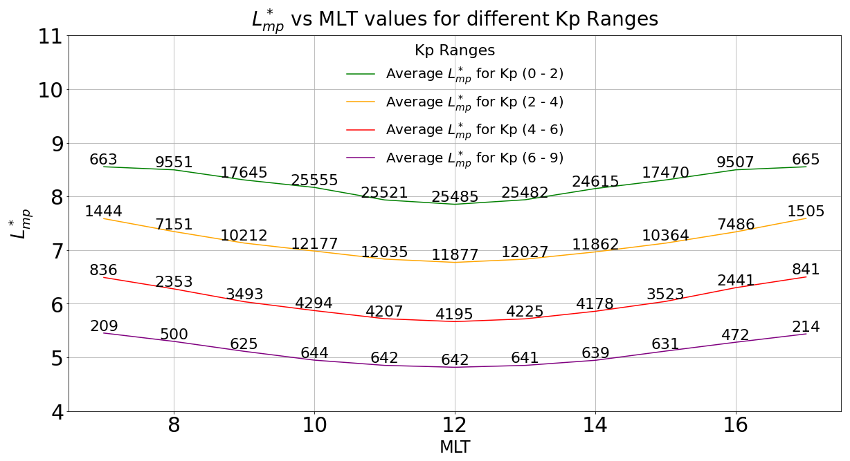
Figure 3 Plot of the global distribution of the dataset, with the curves representing the mean $L_{\mathrm{mp}}^{\ast }$ values, sorted per Kp ranges as a function of the MLT values and the associated number of valid points at each MLT bin.

The magnetopause is considered to be closest at 12:00 MLT, as in the Shue model. To ensure consistency, we filtered out values where the calculated magnetopause is computed as minimal outside of 12:00 MLT. These values arise when inconsistencies occur between the geographical position given by the Shue model and the numerical magnetic field mapping in the T89C model. These cases never exceed a few percent of the value at 12:00 MLT.

The first MLT bin that shows a mean $L_{\mathrm{mp}}^{\ast }$ value is 10:00 MLT, noticeably higher than at 12:00 MLT, with a difference of up to 2 %. We limited the statistical analysis to the data available at 10:00 MLT, ensuring that the dataset predominantly includes magnetopause locations covering MLT values between 10:00 and 14:00. Without this limitation, the varying amount of data per MLT would have introduced bias. For example, the high concentration of values at 12:00 MLT, where most calculable drift shells are located, could distort the results for other MLT bins, resulting in a model that performs well at 12:00 MLT but is less accurate at other MLT bins. Although this approach reduces the size of our dataset, it enhances the significance of the analyzed data. As previously established, the $L_{\mathrm{mp}}^{\ast }$ value at 12:00 MLT serves as a driver for the magnetopause location model. The constructed dataset was thus normalized using this value. Consequently, the updated dataset now consists of the value of $L_{\mathrm{mp}}^{\ast }$ at all dayside MLT bins, normalized by $L_{\mathrm{mp}}^{\ast }$ at 12:00 MLT, for epochs where a valid point exists at 10:00 MLT.

Figure 4 depicts the mean normalized $L_{\mathrm{mp}}^{\ast }$ (denoted ${\stackrel{\mathrm{‾}}{L^{\ast }}}_{\mathrm{mp}}$) and percentile distributions for each Kp range as a function of MLT. The plot depicts in gray the MLT regions below 10:00 MLT, where variations driven by the Kp index are significant. The distribution is flat at around 12:00 MLT, with at most a deviation of under 2 % at 11:00 MLT (and 13:00 MLT) for all Kp values, and the ${\stackrel{\mathrm{‾}}{L^{\ast }}}_{\mathrm{mp}}$ values at 11:00 and 13:00 MLT have a maximum of around 1 %. This can be interpreted as the magnetopause aligning with a specific drift shell in MLT sectors close to noon. Consequently, our model considers this assumption so that for MLT (11:00, 13:00),

$$\begin{array}{}\text{(1)}& L_{\mathrm{mp}}^{\ast }=L_{\mathrm{mp}}^{\ast }\left(\mathrm{MLT}=\text{12:00}\right).\end{array}$$

Additionally, the percentiles show that the Kp index has a significant impact on MLT bins below 10:00 MLT, with the ${\stackrel{\mathrm{‾}}{L^{\ast }}}_{\mathrm{mp}}$ equal to 4 % for Kp between 0 and 2 and the associated percentile reaching up to 5 %. This observation suggests that the Kp index affects the shape of the magnetopause and has the greatest influence on MLT values furthest from 12:00 MLT. Furthermore, variations in ${\stackrel{\mathrm{‾}}{L^{\ast }}}_{\mathrm{mp}}$ at 10:00 MLT are consistent with the Kp dependence of the magnetopause location.

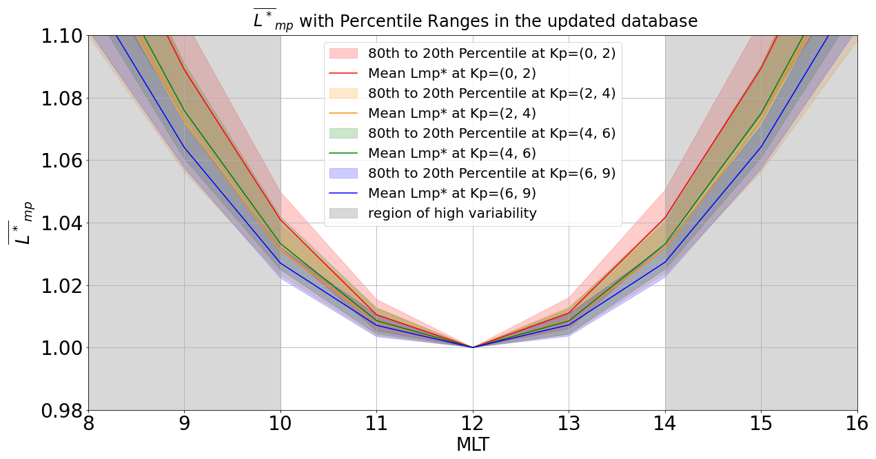
Figure 4 ${\stackrel{\mathrm{‾}}{L^{\ast }}}_{\mathrm{mp}}$ values calculated per Kp range and their corresponding 80th to 20th percentiles, as a function of MLT, with the gray area being the MLT bins of high variability.

In order to quantify the influence of the Kp index on the ${\stackrel{\mathrm{‾}}{L^{\ast }}}_{\mathrm{mp}}$ at MLT values between 10:00 and 14:00 MLT, we analyzed the evolution of ${\stackrel{\mathrm{‾}}{L^{\ast }}}_{\mathrm{mp}}$ within these MLT bins as a function of Kp, as shown in Fig. 5. On the one hand, ${\stackrel{\mathrm{‾}}{L^{\ast }}}_{\mathrm{mp}}$ at 11:00 MLT exhibits a constant evolution as a function of Kp and can thus be considered Kp-independent. On the other hand, the evolution of the ${\stackrel{\mathrm{‾}}{L^{\ast }}}_{\mathrm{mp}}$ at 10:00 MLT as a function of Kp can be fitted. The curve shows a “bump” at Kp of around 5, which has been tracked to be a numerical artifact in the $L_{\mathrm{mp}}^{\ast }$ calculation. This artifact arises from the use of the T89C model, which introduces a Kp class at 5−, 5, and 5+, as compared to the first model version (Tsyganenko, 1989a). At these radial distances and MLT bin, inconsistencies arise with other classes of Kp, as shown in Fig. 6. Consequently, the points at these Kp values have not been considered when building the regression line (Fig. 5). Doing this, the evolution of ${\stackrel{\mathrm{‾}}{L^{\ast }}}_{\mathrm{mp}}$ at 10:00 MLT is well represented at the first order by the simple linear regression in Fig. 5. The impact of the artifact on the regression has been evaluated, and it was found to have no significant effect on the regression line. This conclusion is supported by the minimal differences observed between the two regression lines, shown in red and orange in Fig. 5. This outcome is reasonable, given the consistent behavior of the curve at other Kp values. This regression analysis covers Kp values from 0 to 8, excluding Kp 9 due to the insufficient number of data points available for that range. Nevertheless, the model is extrapolated to Kp 9, ensuring the model's definition across all Kp values.

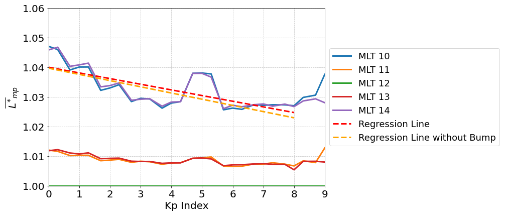
Figure 5 Evolution of ${\stackrel{\mathrm{‾}}{L^{\ast }}}_{\mathrm{mp}}$, sorted by MLT values and plotted as a function of the Kp index. The linear regression lines are shown for the dataset, both with and without the bump included.

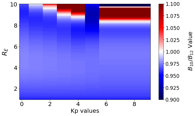
Figure 6 Cartography of the T89C magnetic field model. The y axis represents the radial distances and the x axis represents the Kp index values. The color bar shows the ratio of the value of B at 10:00 MLT to the value of B at 12:00 MLT.

The function of ${\stackrel{\mathrm{‾}}{L^{\ast }}}_{\mathrm{mp}}$ at 10:00 MLT is given by Eq. (2), and its link to the $L_{\mathrm{mp}}^{\ast }$ value is given by Eq. (3).

$$\begin{array}{}\text{(2)}& {\displaystyle }{\stackrel{\mathrm{‾}}{L^{\ast }}}_{\mathrm{mp}}\left(\mathrm{MLT}=\text{10:00}\right)=-\mathrm{0.00188}\times Kp+\mathrm{1.0378}\text{(3)}& {\displaystyle }\begin{array}{rl}{L}_{\mathrm{mp}}^{\ast }\left(\mathrm{MLT}=\text{10:00}\right)& ={\stackrel{\mathrm{‾}}{L^{\ast }}}_{\mathrm{mp}}\left(\mathrm{MLT}=\text{10:00}\right)\\ & \times L_{\mathrm{mp}}^{\ast }\left(\mathrm{MLT}=\text{12:00}\right)\end{array}\end{array}$$

Equations (2) and (3) provide the value of $L_{\mathrm{mp}}^{\ast }$ at 10:00 MLT based on the Kp index. To extend the model to MLT bins below 10:00 MLT, we define an affine function linking the value of the $L_{\mathrm{mp}}^{\ast }$ at 10:00 MLT to $L_{\mathrm{mp}}^{\ast }$ at 11:00 MLT. This function is then extrapolated to other MLT bins, establishing the MLT dependence of the model as follows:

$$\begin{array}{}\text{(4)}& L_{\mathrm{mp}}^{\ast }\left(\mathrm{MLT}\right)=\left(m\cdot \mathrm{MLT}+b\right)\cdot L_{\mathrm{mp}}^{\ast }\left(\mathrm{MLT}=\text{12:00}\right),\end{array}$$

with

$$\begin{array}{}\text{(5)}& {\displaystyle }m=\mathrm{1}-{\stackrel{\mathrm{‾}}{L^{\ast }}}_{\mathrm{mp}}\left(\mathrm{MLT}=\text{10:00}\right)\text{(6)}& {\displaystyle }b=\mathrm{1}-m\cdot \mathrm{11}.\end{array}$$

Figure 7 summarizes the model construction. The model is based on the $L_{\mathrm{mp}}^{\ast }$ value at 12:00 MLT (in green). The flat distribution described by Eq. (1) (in yellow) extends the model to 11:00 and 13:00 MLT. The Kp law, which defines the model's $L_{\mathrm{mp}}^{\ast }$ value at 10:00 MLT (in red), is specified by Eqs. (2) and (3). The affine function (in blue), defining the $L_{\mathrm{mp}}^{\ast }$ value across MLT bins ranging from 06:00 to 10:00, is given by Eqs. (4) to (6). As a result, $L_{\mathrm{mp}}^{\ast }$ at all dayside MLT bins can be expressed as a function of $L_{\mathrm{mp}}^{\ast }$ at 12:00 MLT and the Kp value, as illustrated by Fig. 6.

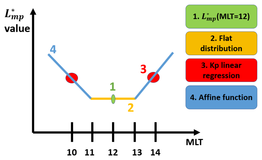
Figure 7 Diagram describing the model construction process, with the $L_{\mathrm{mp}}^{\ast }$ value at 12:00 MLT (green) propagated to 11:00 and 13:00 MLT (yellow), the Kp linear regression giving the $L_{\mathrm{mp}}^{\ast }$ value at 10:00 and 14:00 MLT (red), and the affine function extending the model to other MLT bins (blue).

2.4 Assessing model performance

To assess the performance of our model, we compared its accuracy to the approach outlined in Herrera et al. (2016). This approach is referred to here as the “3D model”. By contrast, the “4D model” explicitly accounts for our new MLT-dependent magnetopause location model. The accuracy of our model was evaluated by comparing its $L_{\mathrm{mp}}^{\ast }$ calculations at each dayside MLT sector to the values in the 20-year dataset on which it is based. The performance was quantified using the root mean square error (RMSE), which provides an interpretable measure of the average deviation between the model's predictions and the dataset values.

Figure 8 presents the RMSE distribution of the 4D model and the 3D model for 06:00 to 18:00 MLT. The RMSE value of the 4D model, between 10:00 and 14:00 MLT, remains at around 0.1, reaching a minimum of zero at 12:00 MLT. This result aligns with the plateau of the $L_{\mathrm{mp}}^{\ast }$ value around 12:00 MLT incorporated into the model's design. Beyond the 10:00–14:00 MLT range, the RMSE increases, reflecting the influence of the linear regression and affine function applied to the MLT bins below 10:00 MLT.

Furthermore, at L^∗ shells, primarily influenced by magnetopause shadowing (L^∗ between 6 and 8), the ΔL^∗ ranges from 0.5 to 0.63 (Fig. 1). In Fig. 8, when the RMSE value is below 0.5, the error remains below the maximal intrinsic uncertainty of the Salammbô L^∗ grid. Therefore, such errors do not significantly impact the modeling. For the 4D model, the RMSE stays under 0.5 for MLT values between 8 and 16 h, demonstrating good accuracy. In comparison, the 3D model maintains an RMSE of below 0.5 only for MLT bins between 10:00 and 14:00, thus inducing complementary uncertainties.

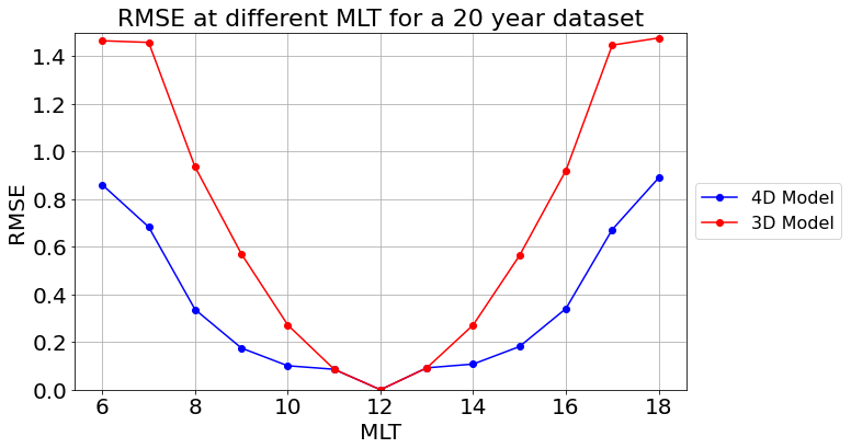
Figure 8 Comparison of the RMSE of the new magnetopause location model (called the 4D model, in blue) and the RMSE of the $L_{\mathrm{mp}}^{\ast }$ value at 12:00 MLT, propagated at every MLT (called the 3D model, in red) as a function of MLT.

Moreover, the RMSE values of the 3D model increase as the MLT moves away from 12:00 MLT, indicating that its fixed $L_{\mathrm{mp}}^{\ast }$ value at 12:00 MLT does not generalize well across other MLT bins. In contrast, the 4D model provides a more accurate representation of the dataset across all MLT bins and geomagnetic activity levels. This improvement stems from its direct dependency on the MLT and Kp index and indirect dependence on solar wind parameters through $L_{\mathrm{mp}}^{\ast }$ at 12:00 MLT.

2.5 Qualitative evaluation of the model of the 2015 St. Patrick's Day storm case study

We then compare our semi-analytical model with the long-term dataset using the March 2015 St. Patrick's Day storm (Baker et al., 2016; Goldstein et al., 2017; Li et al., 2016) as a case study. This analysis seeks to provide a qualitative assessment of the model's behavior during a geomagnetic storm.

The results of the comparison between the model estimations and the effective values are presented in Fig. 9. We provide plots of $L_{\mathrm{mp}}^{\ast }$ for 13:00 MLT (panel a) and 15:00 MLT (panel b) as a function of time. In these plots, the blue dots represent our dataset, while the new model is depicted by the dotted orange line, and the 3D model is displayed as the solid green line. The plot in panel (a), at 13:00 MLT, confirms the flat distribution of $L_{\mathrm{mp}}^{\ast }$ values between 11:00 and 13:00 MLT in the model's construction. Panel (b) demonstrates the 3D model's difficulty to reproduce the dataset values at 15:00 MLT.

While the 4D model generally performs well, there is a slight loss of accuracy in reproducing higher L^∗ values on 15 March 2015 at 10:00  and on 16 March 2015 at 22:00 . During these times, the difference between the data and the model is shown to be less than 0.25. The difference between the dataset's $L_{\mathrm{mp}}^{\ast }$ value, calculated using D_p and B_z, and the model's $L_{\mathrm{mp}}^{\ast }$, based on the Kp law, can be attributed to fluctuations during periods of low geomagnetic activity. During these times, the values of D_p, B_z, and Kp can vary significantly. This variability makes it challenging to accurately model the magnetopause using only the Kp parameter. At L^∗ values ranging from 7 to 8, Fig. 1 demonstrates that differences below 0.5 are not detected by the Salammbô 4D code. Consequently, these minor inaccuracies do not impact the overall modeling results.

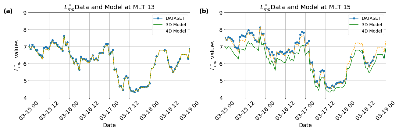
Figure 9 Comparison of the modeled $L_{\mathrm{mp}}^{\ast }$ values of the new magnetopause location model (the dotted orange line), the modeled $L_{\mathrm{mp}}^{\ast }$ value at 12:00 MLT (the solid green line), and the $L_{\mathrm{mp}}^{\ast }$ value of the dataset used to create the model at 13:00 MLT (a) and 15:00 MLT (b) during the March 2015 St. Patrick's Day storm.

The new model demonstrates strong performance during the peak of geomagnetic storms, when the magnetopause is closest to Earth. This is a critical condition for accurate radiation belt modeling. A notable advantage of this semi-analytical model is its ability to reliably generate $L_{\mathrm{mp}}^{\ast }$ values even in data-scarce environments. For example, during the data gap on 18 March 2015, between 12:00  and 24:00 , the model produced values consistent with neighboring observations. This highlights its capability to provide coherent and reliable estimates in the absence of direct measurements.

3 Model evaluation against magnetopause crossing data

The Shue model was originally developed using a magnetopause crossing database compiled up to 1998. Since then, several missions have been launched, providing additional magnetopause crossing data. These recent satellite crossings may be used to validate the new magnetopause model. For this purpose, we choose the catalog of magnetopause crossings of Michotte de Welle et al. (2022) and Nguyen et al. (2022). This catalog uses satellite magnetopause crossings from the Double Star, MMS, Cluster, and ARTHEMIS (THEMIS B and C) missions. The catalog provides extensive MLT coverage, including the dayside, dawn, and dusk sides (as well as high latitudes with Cluster). For each spacecraft, the available data include epochs and the GSM coordinates position of the spacecraft, the ion bulk velocity components (V_x, V_y, V_z), the magnetic fields and its components (B_x, B_y, B_z), the ion density (N_p), and the temperature (T).

To enable a comparison between the new L^∗ model and the magnetopause crossing catalog, adjustments were made. As the magnetopause position model is equatorial, crossings were filtered out to include only those occurring at |Z|≤ 1 in GSM coordinates, focusing on the magnetic equatorial plane. Additionally, the satellite's crossing locations were transformed into L^∗ values, aligning them with the format used in our model for direct comparison.

Figure 10 displays the scatter plot of crossing locations, with the color of the points reflecting the percentage of difference between $L_{\mathrm{mp}}^{\ast }$ values derived from the catalog and those predicted by the 3D model (panel a) and the 4D model (panel b). Panel (a) highlights that the differences between the 3D model and satellite crossings are smaller by up to 15 % at around 12:00 MLT compared to other MLT bins, as expected. This observation supports the accuracy of the magnetopause location model proposed by Herrera et al. (2016) for 12:00 MLT. Panel (b) demonstrates that the 4D model achieves better accuracy across all other MLT bins compared to the 3D model, validating the improvement introduced by the MLT and Kp dependencies in our model.

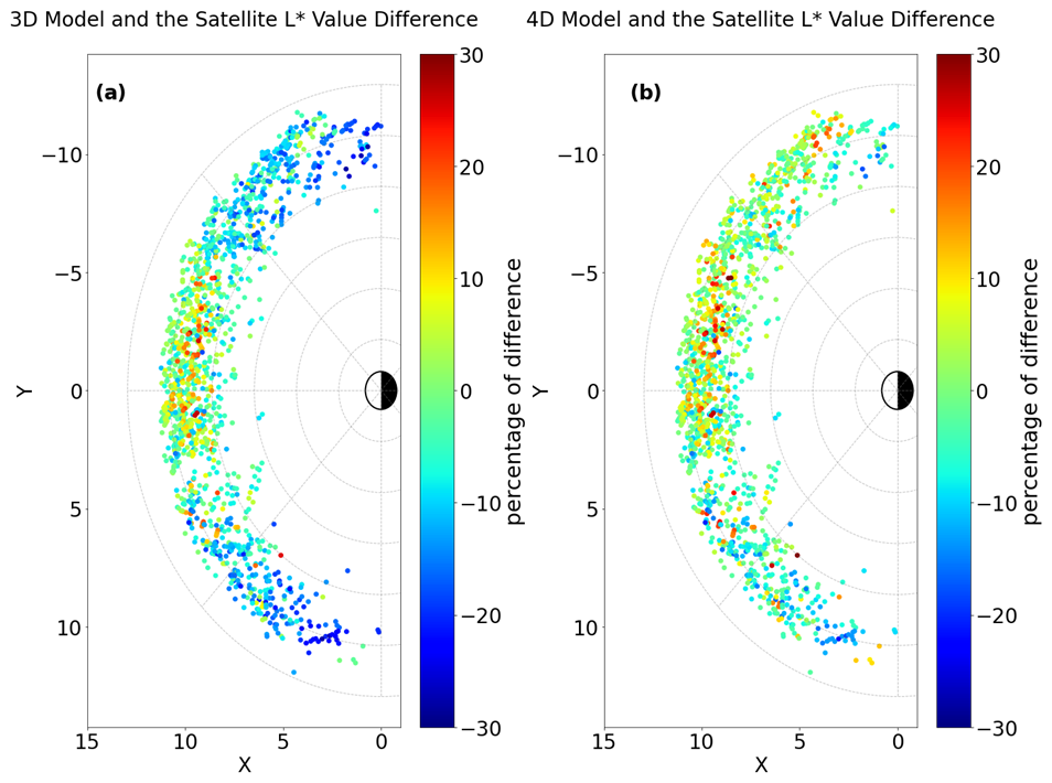
Figure 10 Side-by-side comparison of the relative differences between the satellite's $L_{\mathrm{mp}}^{\ast }$ value and the $L_{\mathrm{mp}}^{\ast }$ value from the 3D model (a) and the relative differences between the satellite's $L_{\mathrm{mp}}^{\ast }$ value and the $L_{\mathrm{mp}}^{\ast }$ value from the 4D model (b). The grid represents dayside MLT bins, with the y=0 axis aligned along the Sun–Earth line. The color of each scatter point corresponds to the percentage of difference between the modeled $L_{\mathrm{mp}}^{\ast }$ value and the satellite crossing $L_{\mathrm{mp}}^{\ast }$ value, as indicated by the color bar.

To evaluate the performance of the 4D model compared to the 3D model, we employed RMSE as the evaluation metric. Figure 11 shows a bar plot comparing the RMSE values between the magnetopause crossing catalog and the two models. The 4D model (in red) exhibits a consistently lower RMSE than the 3D model (in blue) across all MLT values except for 10:00 MLT. At 10:00 MLT, the modeling of $L_{\mathrm{mp}}^{\ast }$ relies on a Kp-dependent linear regression and on an affine function extending the model at other MLT bins. Notably, it demonstrates a lower RMSE in the dawn sector, aligning with the improved accuracy in this region as also suggested by Fig. 10. Overall, the 4D model's lower RMSE indicates superior performance in accurately describing the MLT-dependent variation of the magnetopause location. The absence of an RMSE value at 18:00 MLT is explained by the low number of points used for its calculations in this sector.

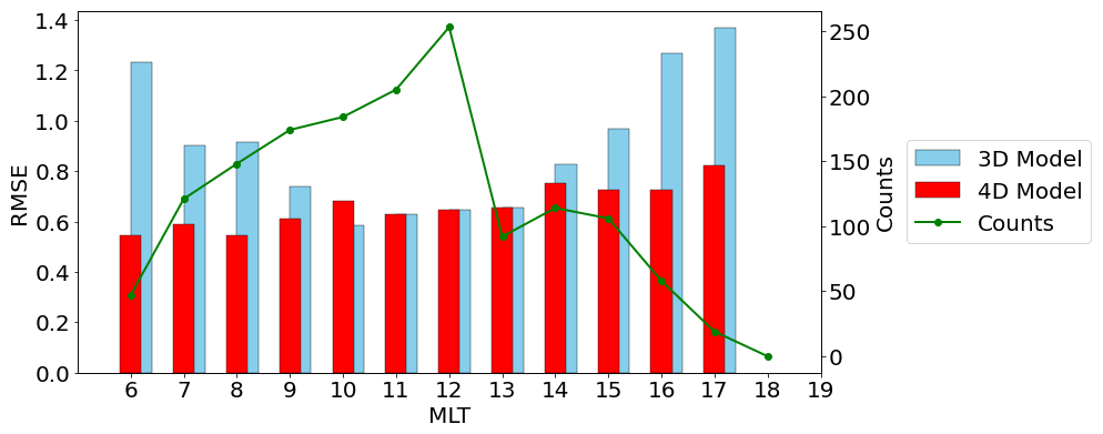
Figure 11 Comparison of the RMSE values (left y axis) for the new 4D model (red) and the 3D model (blue) as a function of MLT, along with the number of points used to calculate the RMSE (right y axis).

The symmetrical nature of the Shue magnetopause model, used as the reference for constructing the dataset, resulted in a symmetrical 4D magnetopause location model. Figure 11 demonstrates that the model has a better accuracy on the dawn sector than in the dusk sector. The dawn–dusk asymmetry of the magnetopause during disturbed times, documented by Dmitriev et al. (2004), suggests that the reliance on a symmetric reference model may have introduced inherent limitations.

Validating the 4D model against the recent magnetopause crossing catalog relies on the assumption that the Shue model remains accurate for all conditions. At 12:00 MLT, this validation indirectly evaluates the Shue model itself. Specifically, a comparison between the predicted distances from the Shue model (converted in L^∗) and recent satellite crossings (also in L^∗), resulted in an RMSE value of 0.65, indicating the existence of inherent uncertainties in the Shue model. Staples et al. (2020) investigated the Shue model's accuracy using satellite data and found it to be reasonably reliable during periods of low geomagnetic activity. However, its reliability decreased under disturbed conditions, with an error margin of ± 1 R_E. While their study focused on distances in R_E, it supports the utility of the Shue model but also highlights potential uncertainties arising from its limitations. These limitations should be considered when interpreting the 4D model's performance, ensuring that any residual discrepancies are understood in the context of the underlying assumptions rather than as flaws in the 4D model itself.

The validation confirms that our new magnetopause location model provides an accurate representation of the magnetopause L^∗ location. Since this model serves as a boundary for the L^∗ parameter in the Salammbô code, its influence is most pronounced on the outermost L^∗ shells of the Salammbô grid. At high L^∗ values, Fig. 1 shows that the L^∗ grid has low refinement, with a spacing of 0.63 between $L^{\ast }=\mathrm{8}$ and $L^{\ast }=\mathrm{7.3}$. The 4D model's RMSE values, ranging from 0.54 at 06:00 MLT to 0.82 at 17:00 MLT, generally fall within this grid spacing. Therefore, the model's error is unlikely to significantly affect the radiation belt modeling in the Salammbô code. Even when the RMSE slightly exceeds 0.63, the resulting impact would be minimal, leading to a shift of at most one grid cell in a Salammbô simulation scheme.

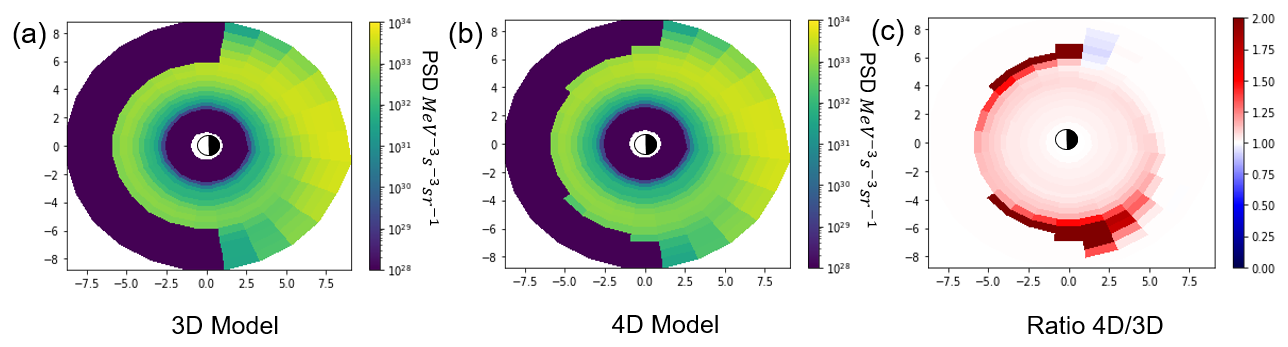
Figure 12 Comparison between the phase space density of a Salammbô simulation at μ=5 MeV G⁻¹ during the geomagnetic storm of March 2015 with the 3D magnetopause model (a), the 4D magnetopause mode (b), and the ratio of the two (c).

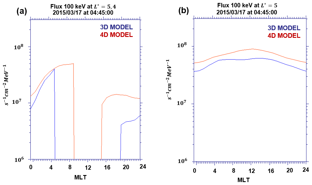
Figure 13 Comparison of FEDO fluxes at the magnetic equator for 100 keV electrons as a function of MLT at a fixed time step during the March 2015 geomagnetic storm, simulated using the Salammbô model. The fluxes are shown for the 3D magnetopause location model (blue) and the new 4D magnetopause location model (red). Panel (a) shows the fluxes at $L^{\ast }=\mathrm{5.4}$ and panel (b) at $L^{\ast }=\mathrm{5}$.

4 Impact of the new magnetopause model in the Salammbô 4D code: the St. Patrick's Day storm in March 2015

The Salammbô 4D code is a modified version of the Salammbô code of Bourdarie et al. (1996) that accounts for the dynamics of low-energy electrons. The boundary condition is derived from THEMIS data (Maget et al., 2015) to which a Gaussian distribution as a function of MLT centered around midnight has been added to account for this added dimension. The code considers the same radial diffusion model used in Boscher et al. (2018) and Brunet et al. (2023). The magnetospheric electric field model used to model the convective transport of particles is the UNH-IMEF Matsui et al. (2013) numerical model. Wave–particle interactions are taken into account using estimation pitch angle and energy diffusion coefficients from the WAPI code of Sicard-Piet et al. (2014) using an MLT-dependent classification of VLF waves. Finally, rapid losses from magnetopause shadowing are implemented such that all particles with an L* greater than L^*, defined by the magnetopause location model, are lost.

A comparison between the new and the previous magnetopause models has been made through the simulation of the March 2015 St. Patrick's Day storm. Results, depicted in Fig. 2, showcase the electron phase space density (PSD) on 17 March 2015 (at 04:45) a few times before the storm's peak. Panel (a) depicts the behavior of the 3D model with an MLT-constant L^∗ value for the magnetopause location equal to $L_{\mathrm{mp}}^{\ast }$ at 12:00 MLT. Panel (b) illustrates the behavior of our novel magnetopause model that considers the MLT dependency and allows a more gradual magnetopause shadowing process on the dayside. The ratio between the new model and the previous one can be seen in panel (c), where the PSD ratio, globally higher than 1, indicates that more particles are lost with the 3D model than with the 4D one. Although the magnetopause shadowing is only applied to the dayside, ratios are also different from 1 in the nightside. This is due to the electric fields that induce a convective transport of particles (both in MLT and in L^*). Panel (c) highlights the importance of an MLT-dependent magnetopause model, where particles lost in the 3D model are transported to the nightside in the 4D model due to this convective transport mechanism.

Figure 3 supports this assumption by showing the omni-directional fluxes at the magnetic equator for 100 keV electrons as a function of MLT on 17 March 2015 at 04:45, based on two Salammbô 4D simulations. The first one uses the 3D magnetopause location model (in blue), while the other one considers the 4D magnetopause location model (in red). Panel (a) illustrates the fluxes of electron at $L^{\ast }=\mathrm{5.4}$, where particles get impacted by the magnetopause shadowing, and panel (b) shows the fluxes of electron at $L^{\ast }=\mathrm{5}$ on a closed drift shell. Both panels illustrate that the 3D model has lower fluxes compared to the 4D one. This means that more particles are lost with the 3D model. In contrast, our 4D model preserves these particles, which are transported deeper into the radiation belts. Consequently, we can state that the use of the 3D magnetopause model on a 4D radiation belt code results in the excessive loss of low-energy particles compared to our new magnetopause model that is MLT-dependent.

5 Conclusions

This study presents a novel semi-analytical model expressing magnetopause location as a function of L^∗ and MLT. This model is specifically designed for MLT-dependent convective and diffusive radiation belt modeling codes, which require the magnetopause position expressed in terms of magnetic parameters to account for the magnetopause shadowing effect. Unlike previous models such as those by Shue et al. (1998) and Lin et al. (2010), which define the magnetopause in Earth radii (R_e), our model provides a more suitable representation for the inner magnetosphere by using L^∗ as a key coordinate. Building on Herrera et al.'s (2016) 3D model at 12:00 MLT, our approach extends coverage to other dayside MLT sectors.

Our model is based on a statistical analysis of L^∗ calculations and was validated against a detailed satellite magnetopause crossing catalog. The results demonstrate accuracy in estimating the magnetopause position in L^∗, particularly in the dawn sector, thanks to our model's dependence on MLT and the Kp index. Our approach shows that an appropriate modeling is one that represents the magnetopause as rather blunt on the dayside but with a clear Kp dependence in other MLT sectors.

The integration of our magnetopause location model into the Salammbô 4D radiation belt model will improve its accuracy. This improvement relies on the L^∗ grid resolution being sufficiently refined to capture particle density variations due to magnetopause shadowing, while also minimizing model errors. Validation against a comprehensive magnetopause crossing catalog confirms the model's reliability. Moreover, the model addresses the challenge of a lack of data, providing a continuous estimation of the magnetopause location. This continuity makes it an excellent fit for radiation belt modeling, where gap-free boundary conditions driving input data are essential. The first integration of the new magnetopause model into the Salammbô 4D code highlights its coupling with the physical processes in the radiation belt dynamic modeling, particularly the convective transport of particles driven by magnetospheric electric fields.

This equatorial magnetopause location model is deliberately tailored for incorporation into MLT-dependent radiation belt codes at the magnetic equator, following Herrera et al.'s (2016) justification (Sect. 2). We prioritized in this work L^∗ and MLT dependency to extend Herrera et al.'s (2016) model. We acknowledge that a more advanced, non-equatorial magnetopause location model could be explored in future research.

Future studies should focus on validating the model through statistical comparisons with in situ satellite data and the satellite trajectories mapping in terms of L^∗ and MLT, incorporated into Salammbô simulations. This approach will enhance our understanding of particle loss processes associated with magnetopause shadowing in the radiation belts.