Leaping and vortex motion of the shock aurora toward the late evening sector observed on 26 February 2023

On 26 February 2023, a shock aurora triggered by an interplanetary (IP) shock was observed in northern Scandinavia at 21 MLT (magnetic local time). Previously, ground-based observations of shock auroras have primarily been conducted on the dayside, where IP shocks hit. However, this study successfully observed the shock aurora on the nightside at 21 MLT. This is the first time the morphology of a shock aurora has been observed on the nightside using ground-based cameras. We introduce the observational results by four ground-based cameras and a magnetometer network in the Northern Hemisphere. Previous observations have shown that shock auroras consist of two types of optical signatures, i.e., diffuse and discrete auroras, with a few minutes of separation. In this study, three distinct signatures were observed with a few minutes of lag: (1) a luminosity enhancement of an arc-shaped green aurora, (2) the appearance of red auroras, and (3) leaping of discrete auroras toward the nightside (anti-sunward) with a vortex-like structure. While red emissions have been previously observed in shock auroras, this is the first time undulating and jumping structures have been discovered. Comparison with equivalent currents estimated from the magnetometer network showed that the first luminosity enhancement occurred within 1 min after the onset of the geomagnetic variation induced by the IP shock, the so-called geomagnetic sudden commencement (SC), and the red aurora observed after the formation of upward field-aligned currents over northern Scandinavia. Furthermore, the propagation speed of the aurora in (3) was on the same order as the solar wind speed in interplanetary space, as reported in previous studies. These newly identified morphological features of the shock aurora provide a valuable insight into how current systems associated with SC propagate toward the nightside.

1 Introduction

Solar wind conditions are among the most crucial parameters contributing to the disturbance of the Earth's magnetosphere (Gonzalez et al., 1994). Accompanying explosive releases of plasma from the Sun, e.g., solar flares and/or coronal mass ejections, the compressed solar wind plasma propagates through interplanetary space as shock waves (Sonett et al., 1964). These shock waves, referred to as interplanetary (IP) shock waves, can induce transient temporal variations in the geomagnetic field through rapid increase in the solar wind dynamic pressure when the IP shock impacts the dayside magnetosphere of the Earth (Araki, 1994; Gosling and Pizzo, 1999). This phenomenon is known as the geomagnetic sudden commencement (SC) (van Bemmelan, 1906; Sano and Nagano, 2021).

SC causes a stepwise increase and bipolar spike in the geomagnetic field variations (Matsushita, 1957, 1960; Wilson and Sugiura, 1961; Araki, 1977, 1994; Slinker et al., 1999). The characteristics of these variations depend on latitude and longitude. According to the Araki model (Araki, 1994), the characteristics are first distinguished between at low and high latitudes. At low latitudes, the horizontal (H) component of the magnetic field shows a stepwise enhancement, while at high latitudes, a bipolar spike occurs with a time lag of a few minutes. These disturbances are called disturbance lower (DL) and disturbance polar (DP), respectively. Furthermore, the bipolar spike of DP is temporally divided into two parts, with the preceding pulse defined as the preliminary impulse (PI) and the following one as the main impulse (MI). PI is associated with a pair of field-aligned currents (FACs) flowing into (out of) the afternoon (morning) auroral zone near the polar cap boundary while traveling anti-sunward. PI is replaced a few minutes later by MI, which corresponds to stationary FACs flowing in the opposite direction from PI. On the afternoon side of the auroral zone and the morning side of the polar cap region, PI is a negative impulse, and MI is a positive impulse, but on the morning side of the auroral zone and the afternoon side of the polar cap region, the polarity is reversed. These features can also be reproduced by computer simulations (Fujita et al., 2003a, b).

Both disturbances are ultimately caused by an intensification of the magnetopause current. The information related to DL propagates globally across the geomagnetic field as the compression carrying FACs at the dawn and dusk edges, appearing almost simultaneously (within tens of seconds) at all magnetic local time (MLT) regions (Araki, 1994). This propagation occurs as an Alfvén wave mode that carries FACs along the geomagnetic field, creating dusk-to-dawn and dawn-to-dusk ionospheric electric fields and other related current systems. DP, especially the PI part, also appears nearly simultaneously at all latitudes. This near-instantaneous appearance is due to the related electric field in the ionosphere, which can propagate almost instantaneously as a waveguide mode (Kikuchi, 2014).

The field-aligned currents and Alfvén waves play a role in particle acceleration along geomagnetic field lines. As a result, auroras associated with SC can be observed. An aurora, known as the shock aurora (Zhou et al., 2003), has actually been observed from space (e.g., Craven et al., 1985; Zhou and Tsurutani, 1999) and ground (e.g., Kozlovsky et al., 2005; Zhou et al., 2009; Liu et al., 2011; Zhou et al., 2017). The shock aurora consists of diffuse and discrete auroras, and their correspondence with geomagnetic variations associated with SC has been widely discussed. For example, Motoba et al. (2009) compared the timing of shock auroras observed by the IMAGE satellite and an all-sky camera at the South Pole station with magnetic field measurements and suggested that the appearance of discrete auroras might be related to the upward FACs during the MI phase. Nishimura et al. (2016) used the magnetometer network in the Northern Hemisphere to obtain the spatial distribution of FACs and their temporal development and compared these with images from an all-sky camera (ASC) in Antarctica. They concluded that the afternoon PI and MI likely correspond to diffuse and discrete auroras, respectively. Motoba et al. (2014) examined a shock aurora at 15 MLT and identified three successive transient arcs (at 557.7 nm) shifting equatorward with an abrupt jump during the PI phase and pointed out that the PI-related FACs might contribute to the formation of these arcs.

The geomagnetic variations and their correlation with auroras have been discussed, but since these variations are one of the phenomena caused by IP shocks, other physical processes are also considered (Zhou et al., 2017). For instance, when the solar wind plasma compresses the magnetosphere, the magnetic field strength increases. As a result, the velocity component of particles perpendicular to the magnetic field lines also increases to conserve the first adiabatic invariant, leading to high-temperature anisotropy. With the increase in temperature anisotropy, electromagnetic waves such as whistler-mode chorus waves and electron cyclotron harmonic (ECH) waves grow nonlinearly (Omura et al., 2015; Omura, 2021). These waves interact with particles (Tsurutani et al., 2001), making them visible as diffuse auroras on the ground (Nishimura et al., 2010; Kasahara et al., 2018; Fukizawa et al., 2018; Nishimura et al., 2020). Additionally, the shear structures in the magnetic field and velocity at the magnetopause caused by IP shocks (Phan and Paschmann, 1996) can create potential drops along magnetic field lines (Haerendel, 2007), increasing the kinetic energy of particles and then making them visible as discrete auroras (Zhou et al., 2017).

The spatiotemporal development of the shock aurora has also been investigated from a wider field of view. According to the global imaging from the satellite, electron and proton auroras propagate anti-sunward at about 4–6 and 10 km s⁻¹ on the duskside and dawnside ionosphere, respectively (Zhou and Tsurutani, 1999; Holmes et al., 2014), and the shock aurora can extend to the nightside. By utilizing multiple scanning photometers installed independently, with approximately 1100 km separation in the evening sector and 900 km in the morning sector, Holmes et al. (2014) demonstrated that the anti-sunward propagation speed of the shock aurora is consistent with the result from satellite observations. The derived propagation speed toward the evening sector was constant on a global scale at about 1–1.5 MLT min⁻¹ (approximately 15–20 km s⁻¹), taking 8 min to propagate from dayside to nightside (20–22 MLT). This is roughly consistent with the 6 min delay of the start of the MI signature observed on the nightside from the onset. Despite various observations and simulations being conducted to clarify the mechanism of shock aurora generation, a comprehensive understanding has yet to be achieved.

To understand the generation mechanism of shock auroras and its correspondence with current systems on a finer spatial scale, it is ideal to use optical observations with ground-based cameras in addition to geomagnetic field measurements from magnetometers. The IMAGE network has multiple ground-based magnetometers across northern Europe (Tanskanen, 2009), allowing for the estimation of ionospheric equivalent currents from magnetic field variations. The term equivalent current means that the current reproduces a magnetic disturbance on the ground, corresponding to the measured disturbance, but does not necessarily reflect the actual ionospheric current. Here we apply the spherical elementary current system (SECS) technique (Amm and Viljanen, 1999). SECS is based on the assumption that sheet-like (height-integrated) divergence-free currents flow at a certain altitude in the ionosphere. Assuming that the horizontal, height-integrated conductivities do not contain strong gradients, the SECS corresponds to height integrated Hall currents, and it can be inferred that upward FACs are at locations with a positive curl of the current and downward FACs are at locations with a negative curl. However, this estimation cannot resolve the structure of FACs with higher spatial resolution than the density of the magnetometer array or the distance from the magnetometers to the ionosphere.

The optical observations of auroras with cameras can provide more detailed information about the current system, such as location and structure, than magnetometers because of their high spatial resolutions. As mentioned above, there have been several examples of observing shock auroras on the dayside, but the shape of the shock aurora has never been captured by ground-based cameras on the nightside. Thus, observations by cameras should be conducted on the nightside to understand how the current system develops as it propagates to the nightside or whether the auroral morphology remains the same after long-distance propagation from the dayside to the nightside. However, it is difficult to observe a shock aurora on the nightside because the arrival of IP shock often causes quick development of the substorm aurora on the nightside right after the SC (Yamauchi et al., 2006; Liu et al., 2013). Only photometer observations with a narrow zonal field of view (FoV) and spatially integrated intensity measurements using a hyperspectral camera have been reported for the nightside ground-based optical observation of the shock aurora so far (Holmes et al., 2014; Belakhovsky et al., 2017).

To summarize our current understanding, there are two forms of shock auroras: diffuse and discrete auroras. However, our knowledge of the differences in propagation speed, local development, forms on the dayside and nightside, and their relationship to geomagnetic signatures remains incomplete. With modern high-spatial- and high-temporal-resolution cameras and a dense magnetometer network in the auroral region, we can observe shock auroras in the nightside sector without the contamination of nightside-driven auroras such as substorm-related auroras.

On 26 February 2023, right after the onset of an SC, the color ASC in Kiruna (65° geomagnetic latitude) located at 21 MLT detected the following signatures: (1) intensification of the pre-existing green arc, (2) appearance of a red diffuse aurora, and (3) secondary green discrete arc. Additionally, the development of the fine structures of the secondary arc was further analyzed using high-speed cameras. The shock aurora weakened within 20 min, and this interval was isolated from the subsequent substorm growth phase. The shock aurora appeared above a densely distributed magnetometer network (IMAGE), allowing for the derivation of the relative location of FACs and auroras with good resolution. Here, we report these combined observations of the shock aurora seen 3 h before the magnetic midnight.

2 Instruments

2.1 All-sky cameras (ASCs)

We have analyzed all-sky color images from commercial digital cameras in Kiruna, Sweden (67.83° N, 20.42° E), and Skibotn, Norway (69.35° N, 20.36° E). In Kiruna, a Sony α7S with a Nikkor 8 mm F2.8 lens was installed at the main building of the Swedish Institute of Space Physics (IRF) and aligned with the geomagnetic north. The camera's ISO sensitivity was set at 4000, and the exposure time was 10–13 s. At Skibotn Observatory, a Sony α6400 with a MEIKE MK-6.5 mm F2.0 lens was used. The ISO was set at 8000, and the exposure time was 8 s. Images were taken every 30 s. These images were used to geolocate and identify broader spatiotemporal variations of the shock aurora. We also used all-sky images from the electron-multiplying CCD (EMCCD) ASC in Tjautjas, Sweden (67.31° N, 20.73° E) (Hosokawa et al., 2023). This camera is equipped with the BG3 glass filter (Samara et al., 2012) to visualize nitrogen emissions and cut bright forbidden emissions at 557.7 and 630.0 nm. The temporal resolution of this camera was 0.01 s (100 frames s⁻¹). The locations of Kiruna, Skibotn, and Tjautjas are shown in Fig. 1h.

2.2 Wide-angle camera (WAC)

A Sony α7SIII with an FE 24 mm F1.4 GM lens was installed at an optical dome in IRF. This camera, referred to as the wide-angle camera (WAC), was oriented in the north-northeast direction at a low elevation with a horizontal field of view of ∼ 73°. The actual observation area is marked by a white rectangle in the last panel of Fig. 2. Data are available only after 18:32 UT due to an operational issue. The WAC recorded video at 30 frames per second, offering a high temporal resolution for visualizing auroral movement within 1 min. The WAC has an image size of 1920 × 1080 pixels, an ISO sensitivity of 80 000, and a $\mathrm{1}/\mathrm{30}$ s exposure time. We averaged 15 images (for 0.5 s) to create snapshots to reduce noise, as shown in Fig. 4.

2.3 Magnetometers

For the detailed analysis in the vicinity of the observed aurora, a selection of magnetometers from the IMAGE network was used in the study. We chose stations north and south of the detected auroras. Data from the IMAGE magnetometers have a 10 s resolution. Additionally, at low latitude, an Intermagnet magnetometer at Huancayo, Peru (12.05° S, 75.33° W), was used. For the estimation of the equivalent current, we applied all the available IMAGE magnetometers, including those from the Greenland east coast and the DTU Space-operated west Greenland magnetometer chain. In addition, we used data from the University of Iceland-operated Leirvogur Magnetic Observatory.

3 Observational results

Figure 1a and b show the interplanetary magnetic field (IMF; the total in black and the z component in red) and solar wind dynamic pressure from the Deep Space Climate Observatory (DSCOVR) at the L1 Lagrange point. A stepwise increase in the IMF intensity and dynamic pressure was observed around 18:40 UT. Other solar wind parameters shown in Fig. A1 were also enhanced, which is a common signature of the IP shock. Figure 1c shows the horizontal (H) component of the geomagnetic field recorded by magnetometers located in Sørøya (SOR), Norway (67.8 MLAT, 21.2 MLT); Tromsø (TRO), Norway (67.0 MLAT, 21.0 MLT); Kilpisjärvi (KIL), Finland (66.3 MLAT, 21.1 MLT); Kiruna (KIR), Sweden (65.1 MLAT, 21.0 MLT); and Huancayo (HUA), Peru (−0.6 MLAT, 14.2 MLT). Their locations, except for HUA, are shown in Fig. 1h. HUA is located on the dayside equator at ∼ 14.2 MLT, which is close to the impact local time of 11–14 MLT. The impact region can be estimated from Fig. A2. All the stations exhibited the SC signature starting at around 19:24 UT. Corresponding to the propagation time from the L1 point to the Earth, there is a time difference of approximately 45 min between the shock wave observed by the DSCOVR satellite at the L1 point and the time when SC was observed on the ground.

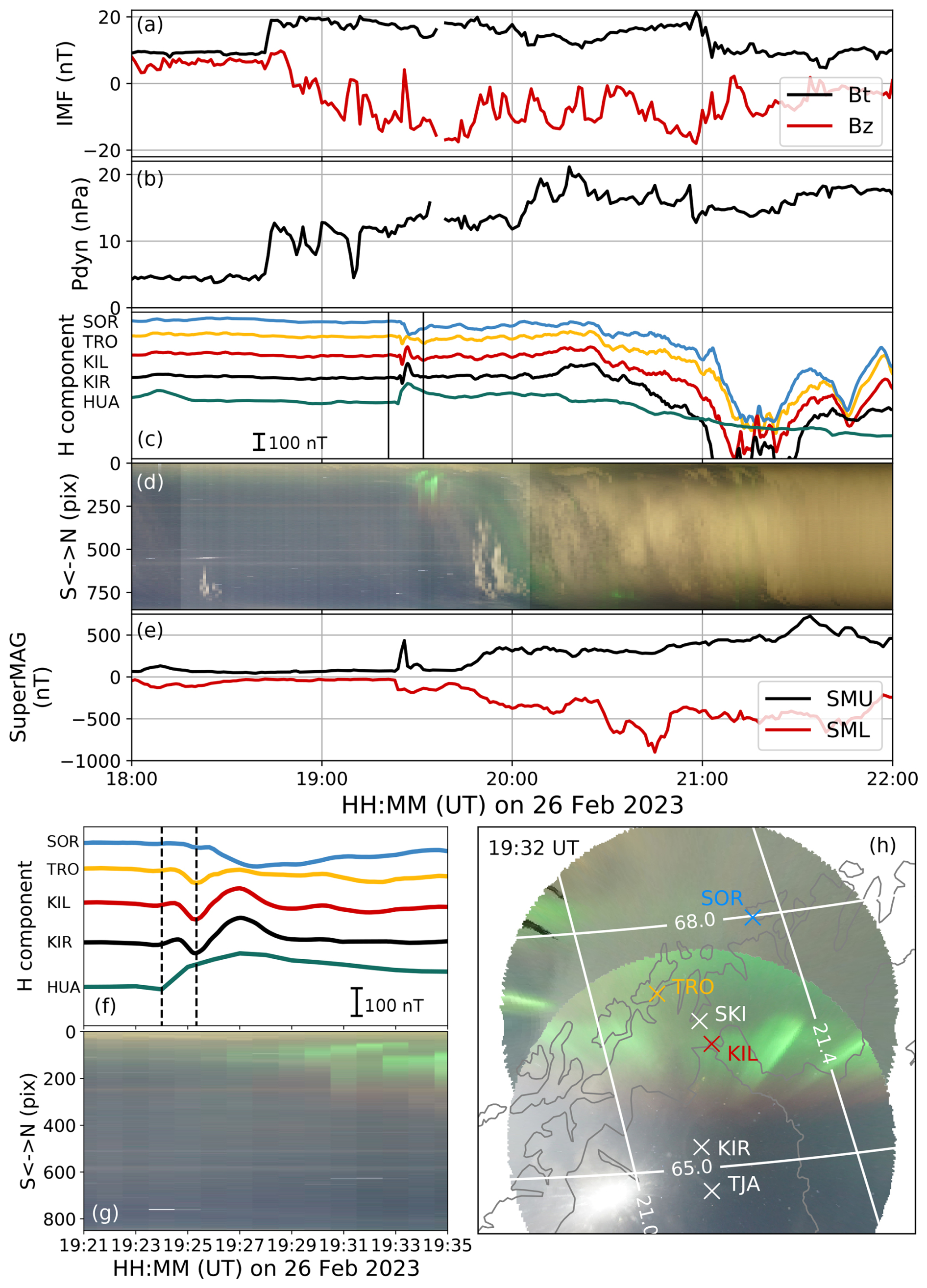
Figure 1 (a–b) The intensity (black) and z component (red) of the interplanetary magnetic field and solar wind dynamic pressure from DSCOVR. (c) Magnetometer data from the stations in the auroral and equatorial regions. A scale of 100 nT is shown in the lower left. (d) North-to-south keogram from the Kiruna ASC. (e) The SuperMAG upper (SMU; in black) and lower (SML; in red) indices. (f–g) Close-up views of panels (c) and (d) from 19:21 to 19:35 UT. Vertical dashed lines indicate the onset of the SC and peak time of the PI. (h) Projection of all-sky images from the Kiruna and Skibotn ASCs. The location of the magnetometers is also shown. The grid lines give the magnetic local time and latitude. There is a time difference of approximately 45 min between the time the shock wave was measured at L1 and the time SC was observed on the ground.

In Fig. 1e, SuperMAG indices (Newell and Gjerloev, 2011; Gjerloev, 2012), upper (SMU) and lower (SML), are plotted. Both SMU and SML values were close to zero before the SC onset. Following the onset, there was a transient increase in SMU and a decrease in SML. All these behaviors indicate that the entire event, from the arrival of IP shock to 20 min after the SC onset, is free from magnetospheric activities initiated in the plasma sheet on the nightside, such as substorms. In the close-up data from 19:21 to 19:35 UT in Fig. 1f, the onset time at ∼ 19:24:00 UT is marked by the left-side dashed line. Similarly, the peak time of the PI at ∼ 19:25:20 UT is also marked by the right-side dashed line. The MI peak was around 19:27:00 UT. From the geomagnetic variations, the ionospheric currents can be estimated, and the gradient in the latitudinal direction suggests that the current intensity became stronger about 3 min after the onset. A detailed estimation of the current system will be introduced later in Fig. 5.

Figure 1d and g show the keogram, the time series of the geomagnetic north–south cross section of the all-sky images from the ASC in Kiruna. Note that the exposure time changed from 10 to 13 s at 19:28 UT. The keograms show that the aurora appeared several minutes after the SC onset and that its intensity gradually increased for the first ∼ 10 min. Then, as indicated by the black arrow, the aurora which appeared initially gradually shifted northward (poleward). In Fig. 1h, all-sky images obtained by the ASCs in Kiruna and Skibotn at 19:32 UT are projected on the map, showing the locations of the magnetometers and cameras. Coordinates with an elevation angle of more than 20° were used for the projection, and the auroral emission layer was assumed to be at 100 km altitude. The projected aurora is found close to the zenith of Kilpisjärvi and Tromsø. In addition, we projected the all-sky image at 250 km altitude, which is available in Fig. A3, to evaluate the altitudinal continuity of the green and red auroras. The location of the red emission at 250 km projection overlaps with the secondary arc projected to 100 km.

Figure 2 shows minute-by-minute all-sky images from 19:23 to 19:34 UT. The upper side of each image is north, and the right side is west and sunward. The solid white line in the first panel indicates the cross-section used to create the keograms shown in Fig. 1. The first all-sky image, taken before the onset of SC, already shows a weak arc-like aurora, circled by the dashed white line in the northeast direction. In this paper, we refer to this aurora as the pre-existing arc. The third all-sky image at 19:25 UT, taken 1 min after the onset, shows that the pre-existing arc had become brighter than before, as indicated by the yellow arrow.

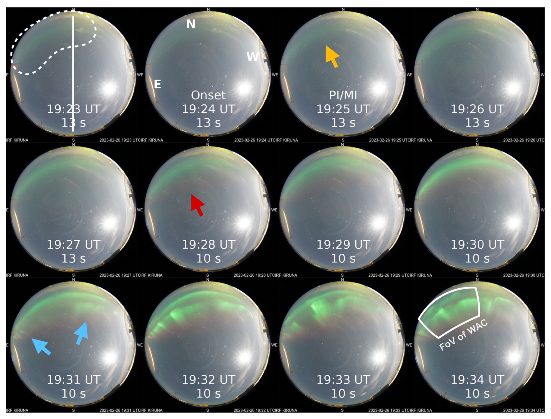
Figure 2 The ASC images from Kiruna during 19:23–19:34 UT on 26 February 2023. The top is the geomagnetic north, and the left is the east. The dashed white region in the first panel shows the pre-existing arc. The appearance of the red aurora and secondary arc is marked by red and blue arrows, respectively. The white rectangle region in the last panel is the FoV of the images shown in Fig. 4.

At 19:31 UT, a discrete green arc with wavy structures was detected southward (equatorward) of the pre-existing arc on both the west (right) and east (left) sides. In this paper, we refer to these arcs as the secondary arc. The secondary arc was brightened at 19:32 UT and subsequently formed a complex structure from west to east. The last four all-sky images (19:31–19:34 UT) show the rapid evolution of the secondary arc and the gradual northward shift in the pre-existing arc.

In addition to these green auroras, a red aurora, as indicated by the red arrow, became visible at 19:28 UT. The red aurora gradually intensified until 19:33 UT and remained in the same location without a distinct structure. In the all-sky images, the red aurora is located southward of both green arcs, but it could also be a high-altitude extension of the secondary arc; i.e., the green and red auroras could be on the same magnetic field lines because the red aurora was projected at the same location of the secondary arcs in Fig. 1h with the assumed emission layer at 250 km.

Due to the 1 min time resolution of the color ASI, it was difficult to examine the propagation of the secondary arc in detail. Thus, we also analyzed a video from the EMCCD ASC in Tjautjas, Sweden (attached as Video S1, Nanjo, 2024a). Snapshots from this video are shown in Fig. 3. Panel (a) was captured at 19:30:00 UT and showed the pre-existing arc outlined by a dotted line near the northern edge of the FoV. Since Tjautjas is located further south than Kiruna, the pre-existing arc appears further north compared to Fig. 2. Then, 1 min later, in panel (b), two spots of the secondary arc began to appear in the northwest, as indicated by the white arrows. These spots propagated eastward, maintaining a spatial gap, as shown in panel (c). Subsequently, in panel (d), another spot indicated by the arrow labeled 3 appeared further east (i.e., ahead in the propagation direction), similarly maintaining a spatial gap from the preceding spots. These observations suggest that the secondary arc propagated from west to east (day to night) in a leapfrog manner. The propagation speed, i.e., averaged leaping speed, in the longitudinal direction, estimated from the video, was about 15–20 km s⁻¹ at the 100 km altitude.

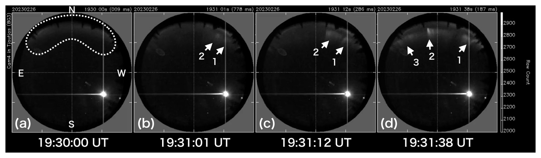
Figure 3 Shock aurora captured by the EMCCD all-sky camera installed in Tjautjas, Sweden. North is to the top, and east is to the left. (a) Pre-existing arc observed at the northern edge of FoV. (b)–(d) Leaping anti-sunward (eastward) propagation of the secondary arc. The bright area in the lower-right corner of FoV is the Moon.

We further examined the fine spatiotemporal evolution of the secondary arc using a 30 Hz video taken by WAC. WAC captured the white rectangle region in the last all-sky image in Fig. 2. Figure 4 shows snapshots from the video. The images obtained from 19:34.12.1 to 19:35:08.1 UT are shown every 8 s. A real-time video of this sequence starting from 19:31:22 UT is provided as Video S2 (Nanjo, 2025b). Note that both the east–west and north–south directions are reversed from the all-sky images in Figs. 2 and 3. The meridian with an azimuth angle of 0° (northward) is shown as a dotted line in panel (a). In each snapshot, two auroral spots in the ASC are visible, with a spatial gap near the center of the image. Both wavy structures gradually folded due to the combination of westward motion on the front side (low-latitude side) and eastward motion on the back side (high-latitude side), as indicated by the white arrows. As this folding developed, these structures consequently formed a vortex shape. Such folding motions are also recognized in the EMCCD ASC mentioned above (Video S1, Nanjo, 2024a) at 19:31:59, 19:33:32, and 19:34:20 UT. These leaping and folding movements of the secondary arc were not detectable with a scanning photometer and are difficult to capture with a camera unless the temporal resolution is less than a few seconds.

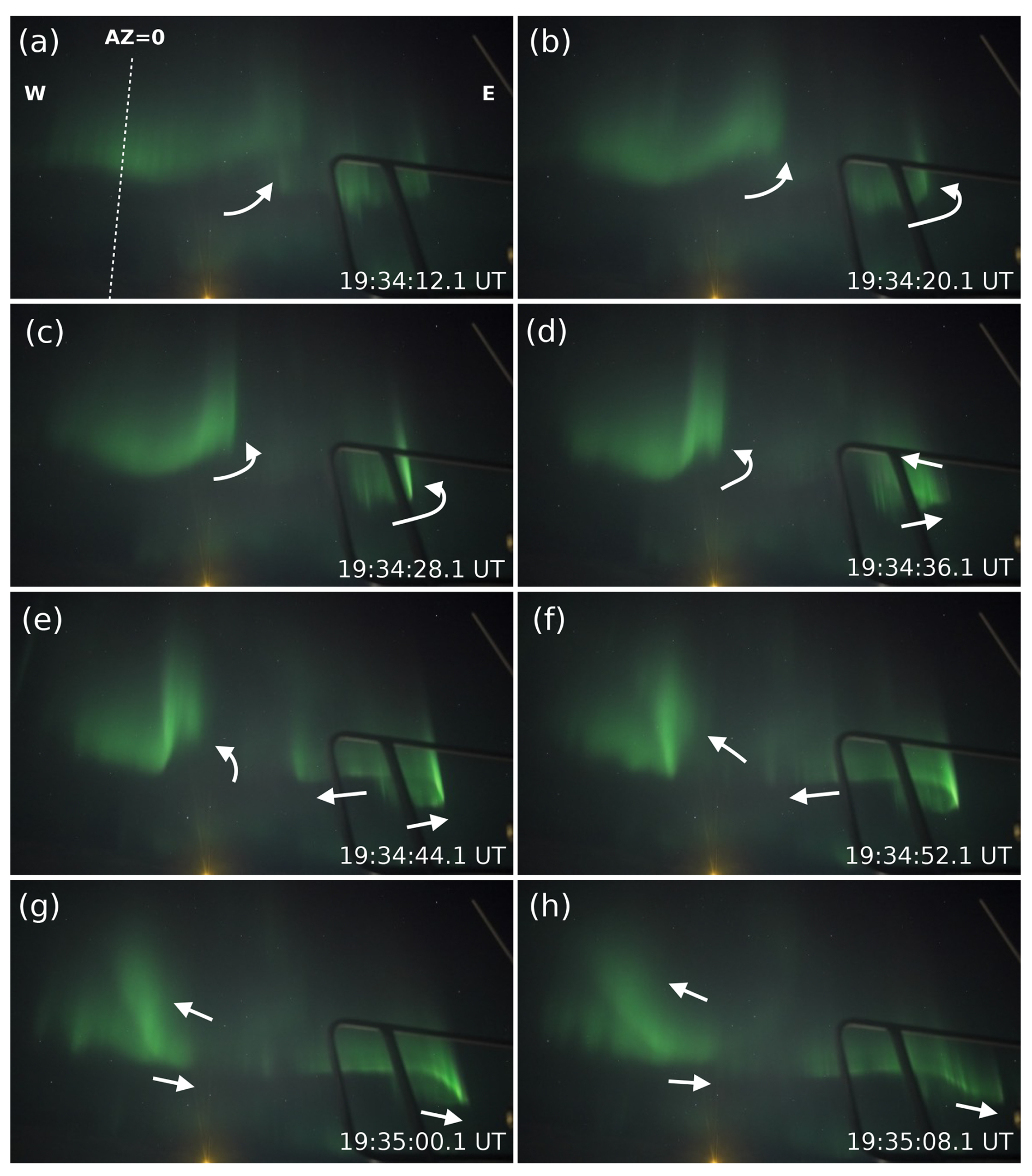
Figure 4 The images captured by WAC from 19:34:12 to 19:35:08 UT. The right side is east (different from the ASC image). The dashed white line in the first panel indicates the meridian, which has an azimuth angle of 0° (toward the geographic north). The white arrows guide the vortex motion.

In the previous paragraphs, we investigate the morphological dynamics of the shock aurora. Here, we derive the ionospheric equivalent currents from magnetometer measurements. Based on data from magnetometers in Greenland and northern Europe and using the spherical elementary current system (SECS) technique (Amm, 1998; Amm and Viljanen, 1999), we created Fig. 5 in the same format as Fig. 4 in Yamauchi et al. (2020). It is important to note that the blue arrows represent measured values, while the red arrows represent interpolated values, which may carry some uncertainty. At the onset shown in panel (a), no significant current flow was observed. However, at 19:26 UT in panel (b), clockwise vortexes corresponding to downward FACs appeared in the latitude range of 70–76°, as indicated by the yellow arrow. Subsequently, from 19:27 UT, a counterclockwise vortex corresponding to upward FACs, indicated by the green arrow, persisted over Scandinavia until 19:31 UT. The intensity of the equivalent currents over Scandinavia was the strongest at 19:27 UT and then showed a decreasing trend.

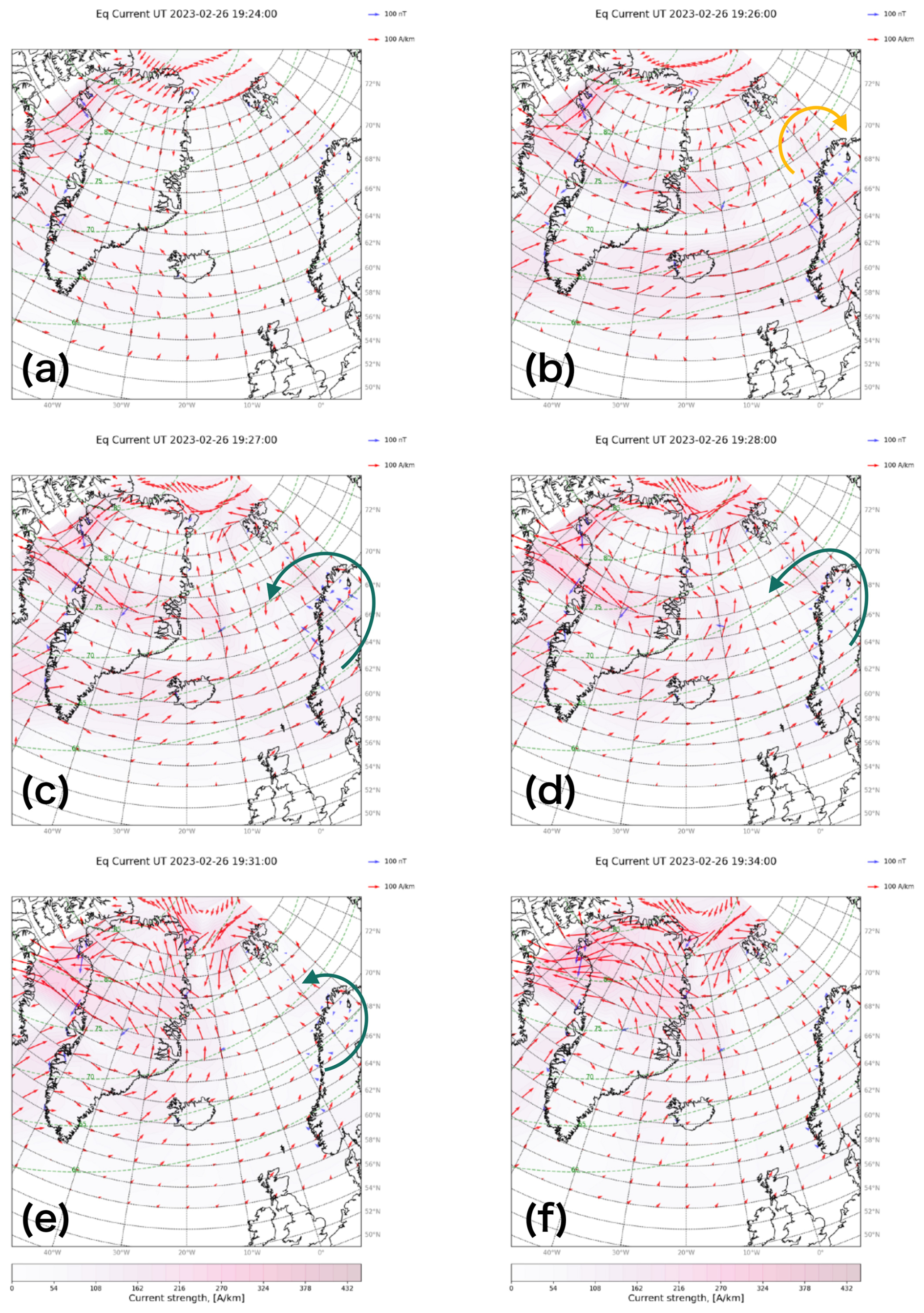
Figure 5 Time variation in the ionospheric equivalent current estimated from magnetometers in Greenland and Scandinavia. No significant current was observed at the onset in panel (a). The clockwise yellow arrow in panel (b) corresponds to downward FAC, and counterclockwise green arrows in panels (c)–(e) correspond to upward FAC. Upward FAC over Scandinavia was weakened from ∼ 19:28 UT.

4 Discussion

A shock aurora was observed by ground-based cameras in the evening sector in response to the SC detected at 19:24 UT during quiet geomagnetic conditions. Their temporal developments are summarized in Fig. 6, which illustrates the locations of the aurora in a polar view.

1. The pre-existing weak arc (green, most likely at 557.7 nm) gradually intensified right after the SC onset and then gradually shifted northward after 19:30 UT.

2. The red aurora (apparently 630.0 nm) without distinct structures gradually appeared widely in the longitudinal direction. This aurora became visible 4 min after the onset, and its location remained stable.

3. The discrete green secondary arc appeared at a few separated spots equatorward of the pre-existing arc at 19:31 UT, i.e., 7 min after the SC onset and 4 min after the peak time of MI. They developed locally to form a spiral-like structure. Subsequently, they were stretched in the east–west direction and connected, as shown in Fig. 6e and f.

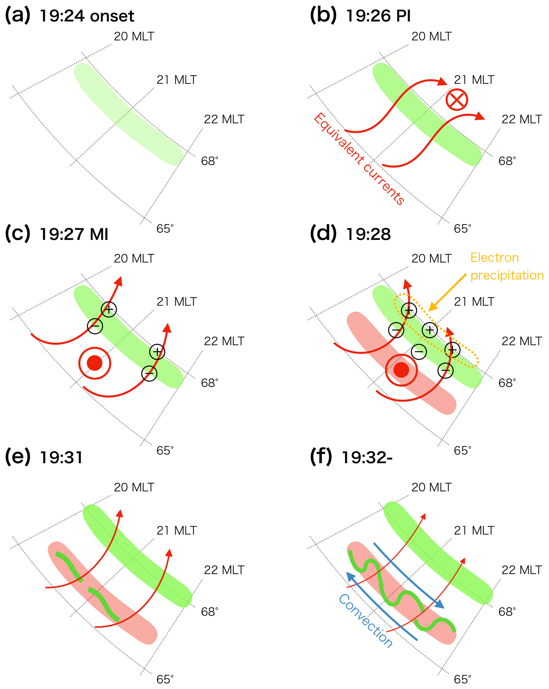
Figure 6 Schematic illustration of the relative locations of the pre-existing arc, red diffuse aurora, and secondary arc. The coordinates of auroras were calculated by assuming the altitudes of green and red emissions were at 100 and 250 km, respectively. The blue arrows indicate the convection directions suggested by the vortex motion of the secondary arc.

There are several unexpected features: (a) three auroral forms appeared instead of the previously reported two forms, PI-related diffuse aurora and MI-related discrete arc; (b) secondary arcs developed as local vortexes at a few spots that leaped eastward (anti-sunward) before forming a connected arc; and (c) the secondary arcs appeared as late as 4 min after the MI peak. This is likely because it was the first time a shock aurora propagating to the nightside was captured using ground-based cameras. Because we did not continuously visualize the aurora from dayside to nightside, it is not necessarily obvious that the observed aurora is a shock aurora. Unfortunately, we currently lack global monitoring of auroras with a sufficient temporal resolution, like the Polar and IMAGE satellites (e.g., Zhou and Tsurutani, 1999; Holmes et al., 2014). However, given that geomagnetic activity and auroral activity were weak before the arrival of this aurora and that the propagation direction was anti-sunward, there is no reason to deny that the observed aurora is the nightside extension of the shock aurora.

The intensity enhancement of the pre-existing arc might be caused by ionospheric currents generated by the SC. According to Fig. 2, the pre-existing arc began to brighten 1 min after the SC onset. This corresponds to the peak of the PI phase, as shown in Fig. 1f. During this time, the equivalent current in Fig. 5b also shows a current system likely induced by the PI phase over Scandinavia. Although the exact mechanism of its emission is unclear, the increased ionospheric current intensity might have caused more precipitation in regions where the aurora was already present and thus conductance was high, resulting in increased brightness. Therefore, the brightening of the observed pre-existing arc may be directly related to the arrival of the SC itself, and it may not be fundamentally important to determine whether this brightening corresponds to the PI or MI phase. According to Figs. 1g and 2, the pre-existing arc shifted northward (poleward) around 19:30 UT. This can possibly be interpreted through latitudinal electric polarization. As shown in Fig. 5, the ionospheric equivalent current over Scandinavia was northward during both the PI and MI phases. This is also represented by the red arrows in Fig. 6. Generally, regions where auroras appear have high conductance. As shown in Fig. 6c, if northward currents cross the pre-existing arc, a spatial gradient in conductance may cause negative charges to accumulate on the lower-latitude (southern) side of the pre-existing arc and positive charges on the higher-latitude (northern) side. To neutralize this asymmetry, electron precipitation may be enhanced in the higher-latitude region of the pre-existing arc, as indicated by the dotted yellow lines in Fig. 6d. Repeating this effect may have caused the pre-existing arc to shift northward. If this is the case, the northward shift may be directly related to the northward current induced by the SC regardless of whether it corresponds to the PI or MI phase.

On the dayside, the first signature of the shock aurora is the diffuse aurora, which appears at lower latitudes compared to the subsequent discrete aurora (Motoba et al., 2009; Liu et al., 2011; Nishimura et al., 2016). However, in this case, the observed pre-existing arc was different from this trend and appeared at higher latitudes compared to the other two signatures. It is also challenging to determine whether the pre-existing arc is a discrete aurora or a diffuse aurora. Diffuse auroras are generated through the interaction between electromagnetic waves and particles in the magnetosphere (Nishimura et al., 2010; Kasahara et al., 2018; Fukizawa et al., 2018; Liu et al., 2023). The 21 MLT region, where this event was observed, is a common area for ECH waves (Ni et al., 2017), which can produce the green line emission (Fukizawa et al., 2020) observed in the pre-existing arc. Nevertheless, due to the lack of available wave measurements, it remains uncertain whether the intensification of the pre-existing arc is due to wave–particle interactions.

The appearance of the red aurora may be attributed to the upward field-aligned currents (FACs) generated in the MI phase. According to Fig. 2, the red aurora began to appear at 19:28 UT. The ionospheric equivalent currents in Fig. 5d indicate a counterclockwise vortex over Scandinavia, suggesting the presence of upward FACs. This may have caused electrons, as carriers of the FACs, to precipitate from the magnetosphere into the ionosphere, producing the red (likely 630 nm) aurora. Therefore, the red aurora may have appeared as a result of the MI current system over Scandinavia. Although the counterclockwise vortex appeared even at 19:27 UT in Fig. 6e, the average lifetime of 630 nm emissions is around 110 s, which might explain this time difference.

The appearance of the secondary arcs may be triggered by the propagation of solar wind plasma across the magnetopause. According to the EMCCD camera data shown in Fig. 3 and the accompanying video, the leaping speed of the secondary arc at an altitude of 100 km was 15–20 km s⁻¹. This corresponds to a longitudinal propagation speed of approximately 1 MLT per minute. Given that the onset region was at 14 MLT, the 7 min delay for the secondary arc to reach Kiruna at 21 MLT is consistent with this speed and aligns with previous observations (Motoba et al., 2009; Holmes et al., 2014; Nishimura et al., 2016). When mapped to the magnetic equatorial plane, this speed translates to several hundred kilometers per second, matching the propagation speed of solar wind plasma.

The currently available dataset does not provide sufficient information to determine the exact process by which the propagation of solar wind plasma triggers the formation of secondary arcs. Proposed mechanisms for the generation of shock auroras include betatron acceleration, magnetic merging, reductions in the mirror ratio, loss cone instability due to adiabatic compression, magnetic shearing, viscous interactions, Alfvén waves, and enhancement of FACs (Zhou and Tsurutani, 1999; Tsurutani et al., 2001; Liou et al., 2002, 2007; Laundal and Østgaard, 2008; Motoba et al., 2009; Zhou et al., 2003, 2009). Combinations of these processes may act together to result in the generation of shock auroras. In our event, as indicated by comparing Figs. 2 and 6, the secondary arcs appeared 4 min after the development of upward FACs during the MI phase. At this time, the intensity of the FACs was decreasing, suggesting that the secondary arcs are not simply brightened by the enhancement of FACs unlike the red aurora. Instead, they likely result from a different mechanism. Given the leaping and vortex motion observed in the secondary arcs, plasma phenomena such as loss cone instability due to adiabatic compression and viscous interactions may play significant roles in their formation.

The optical characteristics of the shock aurora observed in this event, particularly the secondary arcs, still leave some questions unanswered. Given that the propagation speed matched that of solar wind plasma in interplanetary space, it is likely that solar wind plasma played a significant role. Additionally, the pattern of green emissions appearing a few minutes after the red aurora is consistent with observations by Holmes et al. (2014), suggesting that this may be a common feature of shock auroras. As mentioned earlier, the leaping and vortex motion would provide clues about the generation mechanism. However, since this study is based on a single case analysis, it is uncertain whether it represents the average behavior of shock auroras, especially the secondary arcs. Fortunately, modern optical instruments are rapidly improving their sensitivity, and the number of optical stations is increasing. Furthermore, the upcoming SMILE (Solar wind Magnetosphere Ionosphere Link Explorer) mission (Wang et al., 2022), to be launched in 2025, will provide long-term global UV monitoring from almost the same location. Combining its data with improved ground-based optical capabilities will enable systematic studies of shock auroras on the nightside.

5 Conclusions

We observed a shock aurora at 21 MLT using ground-based cameras with color and high spatiotemporal resolution along with ground-based magnetometers. This event exhibited three optical features, unlike the two previously known types of shock auroras. Out of these three auroral forms, the last one (secondary arc) shows an unexpected leaping propagation and folding while remaining fixed in place after leaping. These unexpected features can only be detected with high-time resolution cameras; i.e., scanning photometers cannot reveal them. By combining the estimated ionospheric equivalent currents from the magnetometer network, we discuss the mechanisms behind these emissions. Of the three features, only the red emission might be directly associated with the geomagnetic variations known as PI and MI. This red emission was likely due to upward FACs generated during the MI phase. The initial pre-existing arc was probably influenced more by the arrival of the SC and the resulting northward equivalent currents than by the polarity of geomagnetic changes. The final secondary arcs observed appear to be related not to the current systems induced by the SC but to phenomena resulting from the compression of the magnetosphere by solar wind plasma propagating across the magnetopause.

Appendix A: Supporting figures

A1 Other solar wind parameters

Figure 1 shows the interplanetary magnetic field and solar wind dynamic pressure to indicate the arrival of the interplanetary shock. Additionally, solar wind speed, density, and temperature are included in Fig. A1 below. All parameters increase simultaneously, which can be interpreted as the arrival of the shock wave.

A2 Estimation of the SC onset location

The impact location can be estimated from the global distribution of the geomagnetic disturbance: the DL amplitude (positive step) is maximum near the impact MLT, and the polarity of the DP spike is reversed between the morning side and evening side of the impact MLT (Araki, 1994; Liu et al., 2011). Since the DL amplitude is much larger than the DP amplitude at low latitudes, we can estimate the impact MLT at low latitudes by comparing the amplitude of the H component from magnetometers near the Equator. In Fig. A2, the geomagnetic deviation at HUA, located at ∼ 14 MLT, was outstanding (more than 100 nT) compared to the other Intermagnet low-latitude stations (those showing less than 40 nT). For the DP spike polarity, we have to first consider the difference in the polarity between the auroral/sub-auroral and higher-latitude regions for the same MLT (Araki, 1994; Liu et al., 2011): positive–negative (negative–positive) pair for the morning (afternoon) auroral/sub-auroral latitudes, and this polarity is reversed at the higher-latitude region. To identify the demarcation latitude, we made magnetograms from two stations shown by the solid line (auroral/sub-auroral regions) and the dashed line (higher-latitude region) at 11 and 17 MLT, respectively. With this information, we can estimate the substantial latitudes of both the auroral/sub-auroral DP and higher-latitude DP. The demarcated local time of DP polarity at auroral/sub-auroral latitude is estimated to be between 11 and 13 MLT, i.e., at YKC and FCC, whereas that of the higher latitude is estimated to be between 11 and 15 MLT (no station in between). Altogether, the shock arrival local time is estimated to be 11–14 MLT.

A3 Projection of the all-sky image into an altitude of 250 km

In Fig. 1h, the projection onto the map was made assuming an emission altitude of 100 km in order to understand the location of the green aurora. However, since red auroras occur at higher altitudes than green auroras, the same all-sky image is projected onto an altitude of 250 km in Fig. A3 below. It can be seen that the green auroras in Fig. 1h and the red auroras in Fig. A3 occurred approximately in the same location. From this, we see that the red aurora and the secondary arc are connected in the vertical direction.

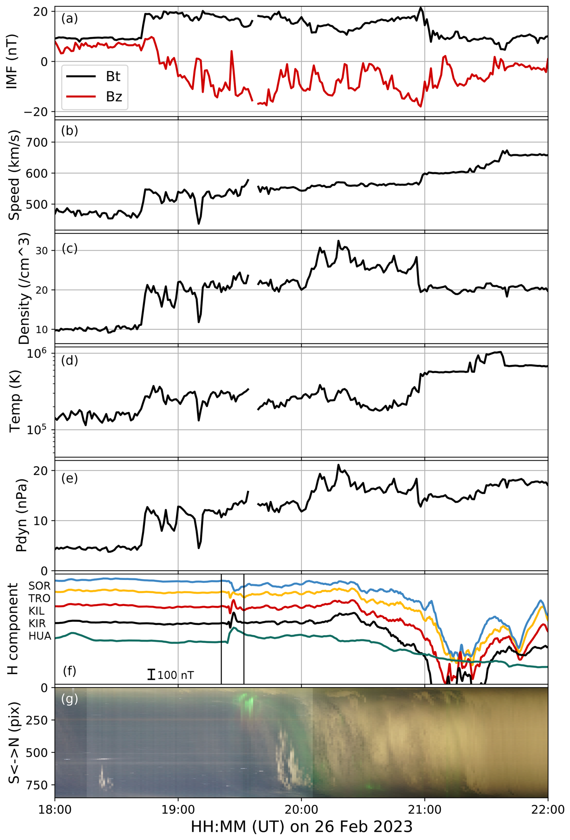
Figure A1 (a–g) The IMF, proton speed, density, temperature, and dynamic pressure from the DSCOVR satellite. The H component of the magnetometers at SOR, TRO, KIL, KIR, and HUA. The north–south keogram from the Kiruna ASC.

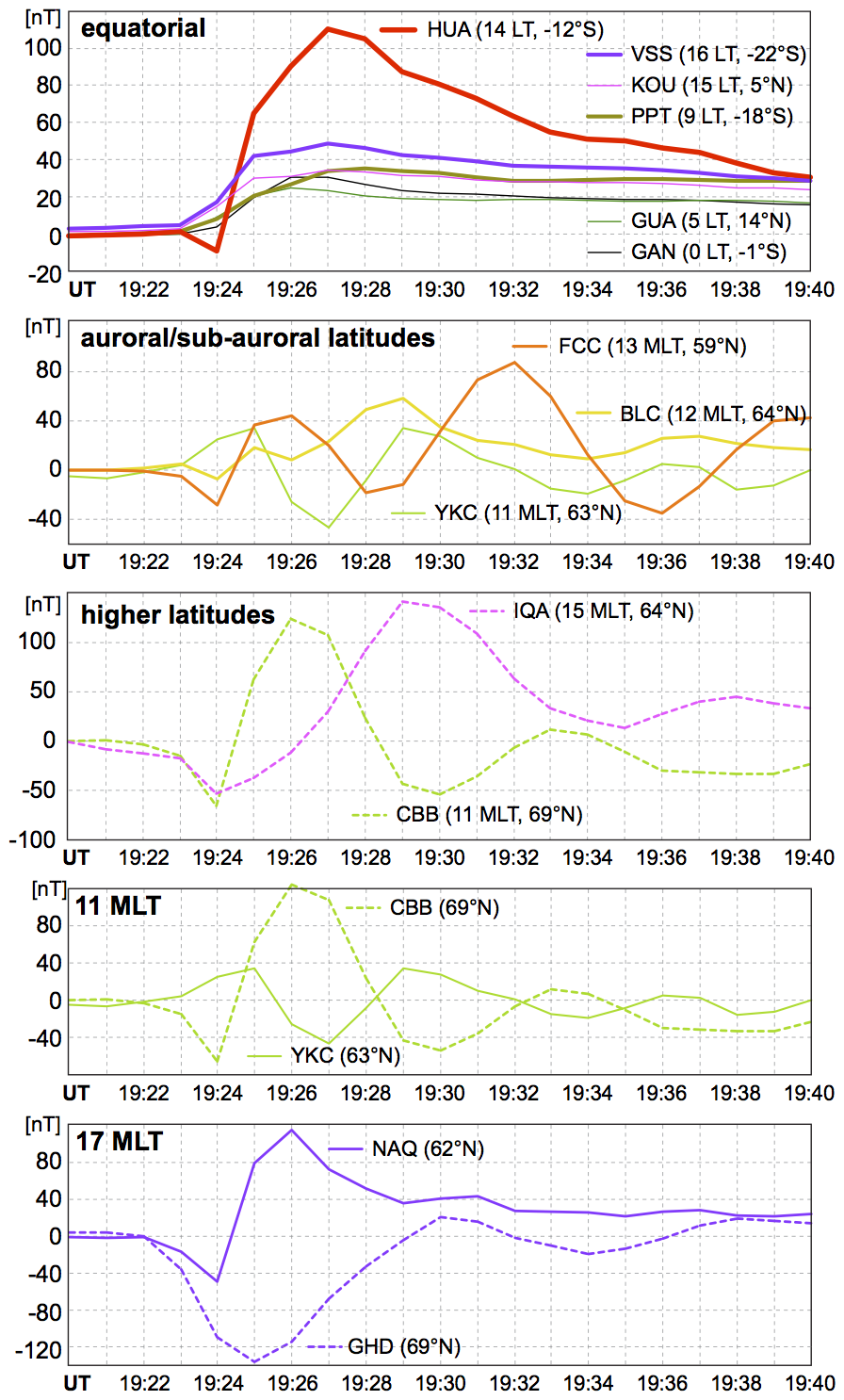
Figure A2 Geomagnetic data for different latitudes in terms of DL and DP signature and for different MLT.

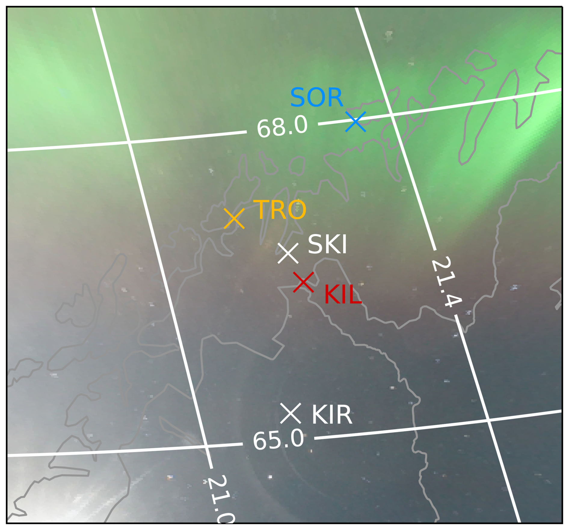
Figure A3 Geographical distribution of the aurora by assuming an emission layer at the 250 km altitude. The red aurora is seen over TRO, SKI, and KIL.