Investigation of the occurrence of significant deviations in the magnetopause location: solar-wind and foreshock effects

Common magnetopause models can predict the location of the magnetopause with respect to upstream conditions from different sets of input parameters, including solar-wind pressure and the interplanetary magnetic field. However, recent studies have shown that some effects of upstream conditions may still be poorly understood since deviations between models and in situ observations beyond the expected scatter due to constant magnetopause motion are quite common. Using data from the three most recent multi-spacecraft missions to near-Earth space (Cluster, THEMIS, and MMS), we investigate the occurrence of these large deviations in observed magnetopause crossings from common empirical models. By comparing the results from different models, we find that the occurrence of these events appears to be model independent, suggesting that some physical processes may be missing from the models. To find these processes, we test whether the deviant magnetopause crossings are statistically associated with foreshocks and/or different solar-wind types and show that, in at least 40 % of cases, the foreshock can be responsible for the large deviations in the magnetopause's location. In the case where the foreshock is unlikely to be responsible, two distinct classes of solar wind are found to occur more frequently in association with the occurrence of magnetopause deviations: the “fast” solar wind and the solar-wind plasma associated with transients such as interplanetary coronal mass ejections. Therefore, the plasma conditions associated with these solar-wind classes could be responsible for the occurrence of deviant magnetopause observations. Our results may help to develop new and more accurate models of the magnetopause, which will be needed, for example, to accurately interpret the results of the upcoming Solar Wind Magnetosphere Ionosphere Link Explorer (SMILE) mission.

1 Introduction

The motion of the magnetopause (MP), the boundary between the Earth's magnetic field and the interplanetary magnetic field (IMF), is driven by pressure variations in the upstream solar wind, changes in the IMF, and flow shear between the magnetospheric and shocked solar-wind plasma (e.g. Sibeck et al., 1991, 2000; Shue et al., 1997; Plaschke et al., 2009a, b; Dušík et al., 2010; Archer et al., 2024a). On the dayside, the boundary attempts to balance the dynamic, plasma (thermal), and magnetic (from the draped field lines) pressures of the shocked solar wind on the magnetosheath side and the magnetic pressure on the magnetospheric side, resulting in the MP changing shape and location in response to upstream condition changes but also to some internal processes (e.g. Shue and Chao, 2013; Archer et al., 2024b). Typically, higher solar-wind total pressures cause the MP to move closer to Earth than its average position, while lower total pressures allow the magnetosphere to expand.

Under strong southward-IMF conditions, magnetic reconnection occurs, where planetary field lines and IMF lines are reconfigured, allowing magnetic flux and energy to be transported around the magnetosphere (Levy et al., 1964; Paschmann et al., 1979, 2013; Petrinec et al., 2022). Due to dayside flux erosion (Aubry et al., 1970; Sibeck et al., 1991; Shue et al., 1997, 1998; Kim et al., 2024) and the transient flux transfer event (Elphic, 1995; Dorelli and Bhattacharjee, 2009; Fear et al., 2017) that result from patchy magnetic reconnection, the MP surface can develop surface waves (Song et al., 1988) and generally moves earthwards from its nominal position. This is due to a decrease in the magnetic field strength in the dayside magnetosphere because of the transport of flux to the nightside and an increase in the field-aligned current strength (e.g. Maltsev and Liatskii, 1975; Wing et al., 2002; Samsonov et al., 2024). As a result, the magnetic pressure balancing the solar-wind pressure is weakened, and the MP is pushed inward.

When the IMF is in quasi-radial configuration, i.e. when the IMF cone angle ϑ_cone between the Earth–Sun line and the IMF vector B_IMF is less than 30 to 45°, the MP is often found sunward of its nominal position (Fairfield et al., 1990; Merka et al., 2003; Suvorova et al., 2010; Dušík et al., 2010; Samsonov et al., 2012; Park et al., 2016; Grygorov et al., 2017).

The foreshock is formed in an extended region upstream of the bow shock due to a fraction of solar-wind particles being reflected at the bow shock and backstreaming along the IMF. As a result, the interaction of solar-wind particles with these backstreamed particles excites instabilities and plasma waves (e.g. Eastwood et al., 2005; Wilson, 2016). A foreshock is present in most IMF configurations, but, in the case of radial IMF, the region forms at and in front of the bow shock nose and becomes most important for MP dynamics by modulating the solar-wind–magnetosphere interaction, e.g. through the occurrence of foreshock transients (e.g. Sibeck et al., 1999; Turner et al., 2011; Archer et al., 2015b; Grimmich et al., 2024c; Kajdič et al., 2024).

An explanation for the expansion under quasi-radial-IMF conditions comes from MHD theory. The reduction and subsequent redistribution of the total pressure of the solar wind by the bow shock and magnetosheath result in a lower pressure on the magnetosphere. This stems mainly from the weaker effect of the field line drape, allowing the MP to move outwards to compensate for the pressure changes (see Suvorova et al., 2010; Samsonov et al., 2012).

The development of Kelvin–Helmholtz instabilities (KHIs) due to shear flows across the MP surface is common (but not exclusive) to northward-IMF configurations and leads to waves on the magnetospheric flanks that contribute to the MP motion (Johnson et al., 2014; Kavosi and Raeder, 2015; Nykyri et al., 2017). Other sources of wave activity and oscillation of the MP independent of the KHI include the flux transfer events mentioned above and wave activity within the foreshock region. The upstream waves in the foreshock can convect through the bow shock and magnetosheath to the MP, generating surface waves and also coupling to waves deep in the magnetosphere (Russell et al., 1983; Luhmann et al., 1986; Fairfield et al., 1990; Russell et al., 1997; Plaschke et al., 2013; Petrinec et al., 2022).

In addition to these external conditions and variations that influence the position of the MP, some studies have shown that internal processes can play a role in the motion of the MP. For example, Machková et al. (2019) have shown that the accurate approximation of the terrestrial magnetic field with an eccentric magnetic dipole shifted by about 500 km from the centre, which yielded a variation in the magnetopause stand-off distance of 0.2 R_E. Effects of magnetospheric currents on MP location have also been reported. The magnetopause distance to the Earth tends to increase for a stronger ring current (e.g. Machková et al., 2019) and decrease with stronger Region-1 Birkeland currents, which accompany the IMF's turning to a southward configuration (e.g. Sibeck et al., 1991).

Empirical models of the MP (e.g. Fairfield, 1971; Formisano et al., 1979; Sibeck et al., 1991; Petrinec and Russell, 1996; Shue et al., 1997, 1998; Boardsen et al., 2000; Chao et al., 2002; Lin et al., 2010; Nguyen et al., 2022a, b) aim to predict the average location of the MP with a given shape under different solar-wind conditions. Thus, in response to the upstream conditions described above, global and quasi-static changes in the boundary can be predicted. However, the models cannot capture the more realistic evolution of the boundary under changing conditions, which leads to the constant motion of the MP, resulting in a natural scatter of model predictions compared to spacecraft observations.

Some of these models focus only on specific regions of the magnetosphere, such as that of Petrinec and Russell (1996) for the near-Earth magnetotail region or that of Boardsen et al. (2000) for the high-latitude regions. The earliest models (e.g. Formisano et al., 1979; Sibeck et al., 1991) use general second-order surface polynomials to describe the surface, while conic sections have become the most widely used functional forms for empirical models. The simplest of these widely used models, such as that of Shue et al. (1997, 1998), assume rotational symmetry that is only influenced by the solar-wind dynamic pressure p_dyn and the IMF component B_z. More complex models, such as those of Lin et al. (2010) or Nguyen et al. (2022a, b), assume a more asymmetric shape, including terms describing the indentation of the surface at high latitudes caused by the cusp and taking into account more parameters affecting the shape and location of the MP (e.g. dipole tilt, magnetic pressure, and IMF magnitude).

Although the use of more complex models improves the prediction accuracy for the MP location, all models still have inherent biases and similar errors around 1 R_E (e.g. Šafránková et al., 2002; Case and Wild, 2013; Staples et al., 2020; Aghabozorgi Nafchi et al., 2024). These errors, which are unable to capture the constant motion around the mean location of the magnetopause, could have several causes. On the one hand, due to the inherently variable nature and spatial structure of the solar wind, which sometimes shows widely different conditions between measurements conducted a few hundred kilometres apart, the conditions measured at L1 (which are often used for MP modelling) may not affect the Earth as expected (Borovsky, 2018a; Burkholder et al., 2020). Several studies like those of Walsh et al. (2019), O'Brien et al. (2023), or Aghabozorgi Nafchi et al. (2024) have shown the complications associated with the propagation of the solar wind to Earth. On the other hand, the studies of Grimmich et al. (2023a, 2024b) have identified specific parameters (such as solar-wind speed, IMF cone angle, Alfvén Mach number, and plasma β) that seem to be responsible for the deviation of the observed MP crossings from the MP models. It is therefore possible that, besides the propagation problem, important mechanisms of the interaction are not yet captured by the models.

For example, high solar-wind speeds appear to lead to an anti-Earthward expansion and outward displacement of the MP from the predicted model location based on the assumption that the higher dynamic pressure in these cases compresses the MP (Grimmich et al., 2023a, 2024b). The foreshock is reported to become stronger (more wave activity and increased occurrence rate of transient events) under high solar-wind speed conditions (Chu et al., 2017; Vu et al., 2022; Zhang et al., 2022; Xirogiannopoulou et al., 2024). Thus, one of these overlooked processes could modify the parameters that affect the MP through the formation of the foreshock region upstream of the Earth's bow shock (e.g. Walsh et al., 2019).

Another point of consideration is the interconnected nature of the solar-wind parameters (e.g. Xu and Borovsky, 2015; Borovsky, 2018b). In general, the solar-wind plasma can be categorized into several types with systematic differences in solar-wind parameters. Most common classification schemes divide the solar-wind plasma into three to four main types: coronal-hole plasma; ejecta and streamer belt plasma; and, from the latter, a subset called sector reversal region plasma (see Xu and Borovsky, 2015; Borovsky, 2020, and references therein). While the ejecta type includes all plasma associated with solar transients, such as interplanetary coronal mass ejections (ICMEs), the other three types can be roughly separated in terms of solar-wind velocity. The coronal-hole plasma is often associated with the “fast” solar wind, with velocities around 550 km s⁻¹; the streamer belt plasma is often associated with the “slow” solar wind, with velocities around 400 km s⁻¹; and the sector reversal region plasma is often associated with the “very slow” solar wind, with velocities around 300 km s⁻¹. The change between the types of solar-wind plasmas then causes synchronous changes in the solar-wind parameters (Borovsky, 2018b).

Therefore, the approach of Grimmich et al. (2023a) may be too simplistic to identify how deviations from MP models arise by identifying the influence of individual parameters responsible for deviations from the MP models. Since Koller et al. (2024) showed that taking different solar-wind types into account improves the classification of magnetosheath ion distributions, it is possible that looking at the response of the MP to different solar-wind types will reveal some missing aspects in current models.

Building on the results of previous studies by Grimmich et al. (2023a, 2024b), in this study, we investigate the relationship between the observed and the modelled MP deviations in relation to the different solar-wind types and quantify the extent to which the foreshock is responsible for the deviations.

2 Data sets and methods

For our investigation, we use the Grimmich et al. (2023b, 2024a) and Toy-Edens et al. (2024a) data sets, which contain observation times and locations of magnetopause crossings (MPCs) from the Cluster (Escoubet et al., 2001, 2021), the Time History of Events and Macro-scale Interactions during Substorms (THEMIS, Angelopoulos, 2008) and the Magnetospheric Multiscale (MMS, Burch et al., 2016) missions in the years between 2001 and 2024. For a comprehensive overview of these data sets, we recommend consulting the relevant publications (Grimmich et al., 2023a, 2024b; Toy-Edens et al., 2024b).

Following the previous studies of Grimmich et al. (2023a, 2024b), we also use the high-resolution OMNI data (King and Papitashvili, 2005) of 1 min resolution to associate all crossings in the data sets with upstream conditions. We take averages from an 8 min OMNI interval preceding each crossing if no more than three data points are missing in that interval for all solar-wind parameters. Otherwise, the crossings are not associated with any upstream data. This handling of the upstream data is identical to that used in the previous studies mentioned (see, for example, Grimmich et al., 2024b, for a detailed discussion). For reference, we also use the 1 min OMNI data from time intervals in the years between 2001 and 2024 where at least one of the three missions is located on the dayside and could potentially observe MPC events.

As the data sets from Grimmich et al. (2023b) and Toy-Edens et al. (2024a) only include dayside events, we have to limit our investigation here to the dayside magnetosphere. Thus, we only use events from the three data sets if they are associated with a positive x component at the observation location in the aberrated Geocentric Solar Ecliptic (aGSE) coordinate system (e.g. Laundal and Richmond, 2016). The aberration is performed by rotating the coordinates around the z axis with an angle computed individually for each crossing, taking into account the mentioned associated solar-wind velocity from the OMNI data set and the Earth's orbital velocity. For cases where the crossings are not associated with OMNI data, we use a mean solar-wind velocity of 400 km s⁻¹ for the calculation.

Furthermore, in the Grimmich et al. (2023b, 2024a) data sets, the crossings are associated with a probability value indicating the certainty of the observed MP identification. We follow the recommendation of previous publications and use only the crossings with probabilities above 0.75, which are considered to be well-identified crossings.

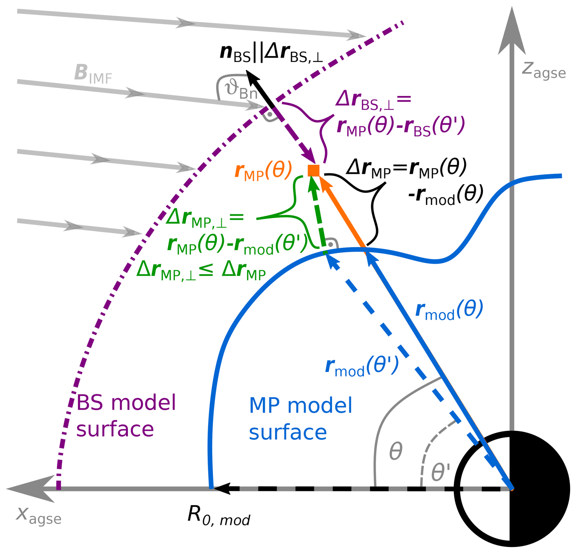
Figure 1 Visualization of the deviation between r_MP and r_mod, an observed MP and the modelled MP location. The sketch is simplified and not to scale and shows only the (x, z) plane, with an arbitrary (indented) MP model in blue. Including the azimuth angle φ next to the zenith angle θ would lead to the generalization described in the text. It can be seen that the difference vector Δr_MP between the spacecraft observation and the modelled surface of the MP would result in greater distances when using θ (the zenith angle of the spacecraft position) in model calculations. The shortest (minimum) distance along the normal to the surface can be found for the angle θ^′ (which can be different from θ) and gives a more physically meaningful representation of the deviation between model and observations (this would also be true for non-indented models). In addition, this sketch shows the geometry of the calculation for the angle ϑ_B,n between B_IMF and the local bow shock normal n_BS, estimated as an anti-parallel vector in relation to the smallest distances from the spacecraft position to a modelled bow shock surface.

Using the associated OMNI data, we calculate the difference between the observed MP position r_MP (i.e. the spacecraft position during a magnetopause crossing) and the position predicted by an MP model r_mod, which we can use to identify events where the model cannot explain the observation. Figure 1 shows a simplified case in the (x, z) plane of the near-Earth space geometry. Here, the simplest approach to calculating the deviation would be to use the zenith angle θ between r_MP and the x axis to determine the location of the MP model r_mod. However, we can see in the sketch that, if we consider the zenith angle θ^′ for the calculation of r_mod, we can determine a perpendicular deviation from the modelled MP surface to the observation point, which is basically the normal displacement of the model MP to the observed crossing. This perpendicular/normal deviation, as seen in the sketch, is shorter than the simple approach calculations and is therefore a more physically meaningful and unbiased difference between r_MP and r_mod.

To describe this physically meaningful difference in a 3D space, we consider all possible θ and φ angles and take the angles θ^′ and φ^′, which yield the smallest deviation from the observed MP location, even though these may not be the angles that describe the observed location. We minimize the term

$$\begin{array}{}\text{(1)}& \mathrm{\Delta }r=|{\mathit{r}}_{\mathrm{MP}}-{\mathit{r}}_{\mathrm{mod}}(\mathit{\theta },\mathit{\phi }\left)\right|,\end{array}$$

where φ is the azimuth angle between the projection of r in the (y, z) plane and the positive z axis.

By comparing the absolute values of r_MP and r_mod, we can also see whether the observed location corresponds to a point further earthward ($\left|{\mathit{r}}_{\mathrm{MP}}\right|<\left|{\mathit{r}}_{\mathrm{mod}}\right|$) or further anti-earthward ($\left|{\mathit{r}}_{\mathrm{MP}}\right|>\left|{\mathit{r}}_{\mathrm{mod}}\right|$) than the model prediction. In the following, we refer to the events occurring further earthward as overestimated MPC and those occurring further anti-earthward as underestimated MPC. For example, the sketch in Fig. 1 illustrates an underestimated MPC.

In this study, we calculate the perpendicular deviation of the MP observation for two different MP models. We use the simple and widely used Shue et al. (1997, 1998) model, hereafter SH98, which describes the MP surface in a rotational symmetry with the function

$$\begin{array}{}\text{(2)}& r_{\mathrm{SH}\mathrm{98}}=R_{\mathrm{0},\mathrm{SH}\mathrm{98}}{\left({\displaystyle \frac{\mathrm{2}}{\mathrm{1}+\cos \mathit{\theta }}}\right)}^{\mathit{\alpha }},\end{array}$$

where R₀ is the magnetopause stand-off distance, and α is the so-called flaring parameter. Since the SH98 model neglects asymmetries in the MP surface, the influence of the dipole tilt angle ψ on the MP shape, and also the prominent indentation feature associated with the cusp regions of the magnetosphere, we will also present results using the relatively new Nguyen et al. (2022b, a) model, hereafter N22b. This model incorporates the above features, and, while similar to the SH98 model in its basic zenith angle function, the IMF dependence in the MP stand-off distance is different, showing a weaker effect on MP motion under a changing IMF. The functional form of the N22b model is described by

$$\begin{array}{}\text{(3)}& r_{\mathrm{N}\mathrm{22}\mathrm{b}}=R_{\mathrm{0},\mathrm{N}\mathrm{22}\mathrm{b}}{\left({\displaystyle \frac{\mathrm{2}}{\mathrm{1}+\cos \mathit{\theta }}}\right)}^{\mathit{\beta }}\left(\mathrm{1}-q(\mathit{\theta },\mathit{\phi },\mathit{\psi })\right),\end{array}$$

where $q(\mathit{\theta },\mathit{\phi },\mathit{\psi })$ is the term describing the indentation of the surface near the cusp influenced by the dipole tilt angle ψ. The flaring parameter of the N22b model β is also influenced by the dipole tilt.

Since currents from the inner magnetosphere, such as the ring current, may have an effect on the position of the MP and, thus, bias our statistics, we have tried to eliminate these influences from our data. We use the calculation presented in Machková et al. (2019) to modify the model output r_mod with the pressure-corrected Disturbance Storm-Time Index (Dst; Burton et al., 1975; Nose et al., 2015). The Dst gives information on geomagnetic activity associated with horizontal magnetic field deviations and can indicate ring current activity and, thus, be used to limit the effects of the ring current.

We can use the minimization of Eq. (1) with the vector r_BS pointing to the surface of a bow shock model (instead of the vector pointing to an MP model surface) to obtain an estimate of the bow shock normal in the vicinity of the MPC observation. The vector $\mathrm{\Delta }{r}_{⟂}=|{\mathit{r}}_{\mathrm{MP}}-{\mathit{r}}_{\mathrm{BS}}({\mathit{\theta }}^{\prime },{\mathit{\phi }}^{\prime }\left)\right|$ for the optimal combination of $({\mathit{\theta }}^{\prime },{\mathit{\phi }}^{\prime })$ from this new minimization should then be roughly aligned with the normal of the model bow shock surface upstream of the MPC observation. Here, we use the Chao et al. (2002) model (CH02) and therefore define the bow shock model normal associated with each MPC as

$$\begin{array}{}\text{(4)}& n_{\mathrm{BS}}={\displaystyle \frac{{\mathit{r}}_{\mathrm{MP}}-{\mathit{r}}_{\mathrm{CH}\mathrm{02}}({\mathit{\theta }}^{\prime },{\mathit{\phi }}^{\prime })}{|{\mathit{r}}_{\mathrm{MP}}-{\mathit{r}}_{\mathrm{CH}\mathrm{02}}({\mathit{\theta }}^{\prime },{\mathit{\phi }}^{\prime }\left)\right|}}.\end{array}$$

We choose the sign of n_BS so that n_BS points to the Sun (i.e. the x component is always positive).

The angle ϑ_B,n is defined as the angle between the computed normals n_BS and the IMF vector B_IMF associated with the magnetopause observation. Typically, the region upstream of the quasi-parallel bow shock (${\mathit{\vartheta }}_{B,n}<\mathrm{45}$°) is associated with the foreshock, while no foreshock activity is expected upstream of the quasi-perpendicular bow shock (${\mathit{\vartheta }}_{B,n}>\mathrm{45}$°). However, the foreshock also extends into the quasi-perpendicular region, and, in some cases, ${\mathit{\vartheta }}_{B,n}<\mathrm{60}$° is used to define the boundary of the active foreshock region (Wilson, 2016; Karlsson et al., 2021). The angle ϑ_B,n can therefore be used to estimate whether the crossing is observed behind the quasi-parallel or quasi-perpendicular bow shock and can thus be associated with foreshock activity.

An alternative to determine whether the spacecraft observation is behind a quasi-parallel or quasi-perpendicular shock is given in Petrinec et al. (2022). The authors take advantage of the fact that the IMF cone angle is identical to ϑ_B,n in the subsolar magnetosphere and map this cone angle to other regions with the clock angle separation between the spacecraft location and the IMF to the corresponding position of the observation. Explicitly, their parameter q is calculated with

$$\begin{array}{}\text{(5)}& \begin{array}{rl}q& =\cos \left({\mathit{\vartheta }}_{\mathrm{cone}}\right)\cos \left({\mathit{\vartheta }}_{\mathrm{clock},\mathrm{IMF}}-{\mathit{\vartheta }}_{\mathrm{clock},\mathrm{sc}}\right)\\ & ={\displaystyle \frac{B_x}{\left|B_{\mathrm{IMF}}\right|}}\cdot \cos \left(\arctan \mathrm{2}\left({\displaystyle \frac{B_y}{B_z}}\right)-\arctan \mathrm{2}\left({\displaystyle \frac{y_{\mathrm{sc}}}{z_{\mathrm{sc}}}}\right)\right),\end{array}\end{array}$$

where B_x, B_y, and B_z are the components of B_IMF, and y_sc and z_sc are the spacecraft position components. This parameter gives a value between −1 and 1, where q<0 indicates that the spacecraft is behind the quasi-perpendicular shock, and q>0 indicates that it is behind the quasi-parallel shock. Both methods are in agreement in up to 80 % of our cases.

We are aware of the fact that this estimate of ϑ_B,n certainly does not give the angle at the bow shock from which the plasma came to influence the MP. Therefore, we use our estimates together with the q value results from Eq. (5), and, when filtering for shock activity, we use only the result from our data sets where both estimates indicate the desired condition. This approach should minimize errors arising from normal and subsequent angle calculations. Taken together, the MPCs in this study are expected to be observed behind the quasi-parallel bow shock and thus in the foreshock region when ${\mathit{\vartheta }}_{B,n}<\mathrm{45}$° and q>0.

In addition, we use the classification scheme introduced in Xu and Borovsky (2015) using the IMF magnitude $\left|{\mathit{B}}_{\mathrm{IMF}}\right|$, the solar-wind ion velocity $\left|{\mathit{u}}_{\mathrm{sw}}\right|$, the solar-wind ion density n_ion, and the solar-wind ion temperature T_ion to group the crossings according to the different solar-wind types with empirically determined thresholds: ejecta (EJC), coronal-hole origin (CHO), streamer belt origin (SBO), and sector reversal region (SRR) (see Xu and Borovsky, 2015).

Transient phenomena such as interplanetary coronal mass ejections (ICMEs) are associated with the EJC type, which is typically described by high IMF magnitudes, intermediate solar-wind velocities, and low Alfvén Mach numbers and plasma βs. High solar-wind speeds with intermediate IMF magnitudes, Alfvén Mach numbers, and plasma β describe the CHO-type solar wind (often referred to as the “fast” solar wind), which originates from open magnetic field lines in the solar corona (coronal holes). The SBO type (often referred to as the “slow” solar wind) originates from regions between the edge of coronal holes and streamer belts and can be described in terms of intermediate solar-wind velocities, IMF magnitudes, Alfvén Mach numbers, and plasma β. Finally, the SRR types (sometimes referred to as “very slow” solar wind) associated with the top of helmet streamers, which are cusp-like magnetic loops in the solar corona, can best be described with low solar-wind velocities and IMF magnitudes and high Alfvén Mach numbers and plasma β (see Xu and Borovsky, 2015; Borovsky, 2018b, 2020; Koller et al., 2024, and references therein). Table 1 shows the median values $\stackrel{\mathrm{̃}}{X}$ and the median absolute deviation, defined as the median of $|X_i-\stackrel{\mathrm{̃}}{X}|$, where X_i denotes the individual data points, for different solar-wind parameters extracted from our OMNI data selection, falling into the four classes to further quantify the above descriptions.

Table 1 Median values with median absolute deviation values of different solar-wind plasma parameters in the four classes of solar-wind plasma from Xu and Borovsky (2015). The parameter values are extracted from the OMNI data set between the years 2001 and 2024.

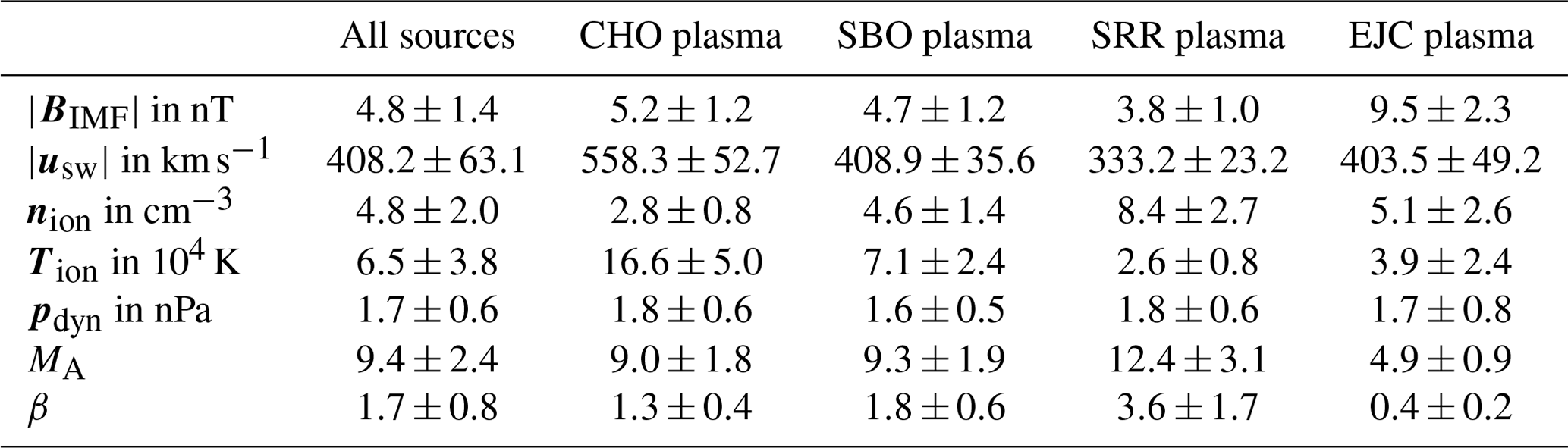
The parameters p_dyn, M_A, and β are derived variables and are therefore inherently connected to the four param3ters $\left|{\mathit{B}}_{\mathrm{IMF}}\right|$, $\left|{\mathit{u}}_{\mathrm{sw}}\right|$, n_ion, and T_ion.

The threshold-based definition of the classes leads to problems near the class boundaries, which could lead to false classifications. To prevent these edge cases from skewing our statistics, for each class, we applied additional thresholds slightly above and below the thresholds given in Xu and Borovsky (2015). We arbitrarily chose the thresholds in such a way that 5 % of each class was identified as an edge case in the classification of our entire OMNI data set.

Since the classification scheme of Xu and Borovsky (2015) does not include information about the orientation of the IMF, which is an important factor for the response of the MP, we extended the four categories to include information about non-radial northward (ϑ_cone>30° and $\left|{\mathit{\vartheta }}_{\mathrm{clock}}\right|<\mathrm{90}$°), non-radial southward (ϑ_cone>30° and $\left|{\mathit{\vartheta }}_{\mathrm{clock}}\right|>\mathrm{90}$°), and quasi-radial IMF (ϑ_cone<30°). This gives a total of 12 different solar-wind categories that can be associated with MPC observations.

Table 2 Number of usable MPCs in the three data sets divided into separate subsets for different magnetospheric regions. The regions are divided according to the latitude and longitude angle (see text for details) into the equatorial subsolar region, the high-latitude subsolar region, the equatorial flank regions, and the high-latitude flank regions. The table also gives a comparison between overestimated and underestimated MPCs in each data set and subset as percentages of the original set. The expanded and overestimated MPCs are identified for two different MP models (SH98 and N22b).

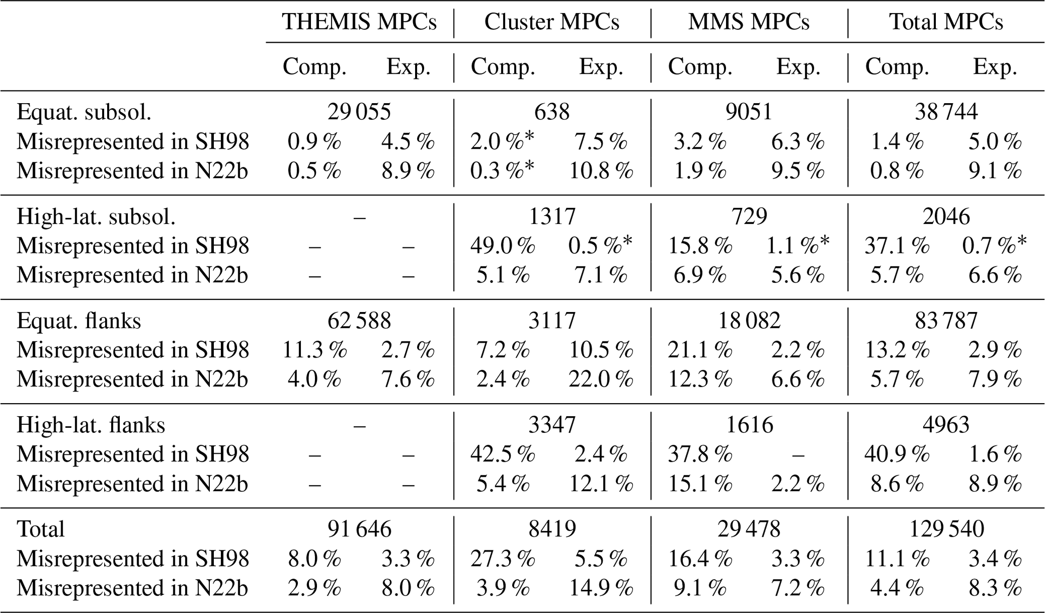
^∗ These subsets have too few observations; therefore, the results from them are most likely unreliable.

3 Results

In the following, we only consider the crossing events from the three data sets in our analysis if all relevant parameters are determined, i.e. if we have values for $\mathrm{\Delta }{r}_{⟂,\mathrm{SH}\mathrm{98}}$, $\mathrm{\Delta }{r}_{⟂,\mathrm{N}\mathrm{22}\mathrm{b}}$, and ϑ_B,n and reliable classification results from the modified Xu and Borovsky (2015) scheme. This leaves us with 129 540 crossing events in a combined data set to examine. The exact composition of this combined MPC data set from the three missions can be found in Table 2. Note that we have not grouped multiple crossings that are close in time and space, as is often done to fit MP models. We are aware that this may lead to a bias in our distributions. However, due to our normalization, this should not affect our results.

In addition, we separate this large combined data set into four distinct regions of the magnetopause over the aGSE latitude ϕ and longitude λ: (1) subsolar crossings observed in the region where $\left|\mathit{\lambda }\right|<\mathrm{30}$° and $\left|\mathit{\varphi }\right|<\mathrm{30}$°; (2) high-latitude subsolar crossings observed in the region where $\left|\mathit{\lambda }\right|<\mathrm{30}$° and $\left|\mathit{\varphi }\right|\ge \mathrm{30}$°; (3) near-equatorial flank crossings observed in the region where $\left|\mathit{\lambda }\right|\ge \mathrm{30}$° and $\left|\mathit{\varphi }\right|<\mathrm{30}$°; and (4) high-latitude flank crossings observed in the region where $\left|\mathit{\lambda }\right|\ge \mathrm{30}$° and $\left|\mathit{\varphi }\right|\ge \mathrm{30}$°. The total number of MPCs observed in these regions can also be found in Table 2.

Based on the results of Case and Wild (2013) and Staples et al. (2020), we consider ±1 R_E deviations between observed and model MP locations to be typical errors in the models. Thus, deviations in Δr_⟂ up to ±1 R_E are considered to be part of the constant motion of the MP surface, which empirical models cannot capture, showing agreement between model and observation.

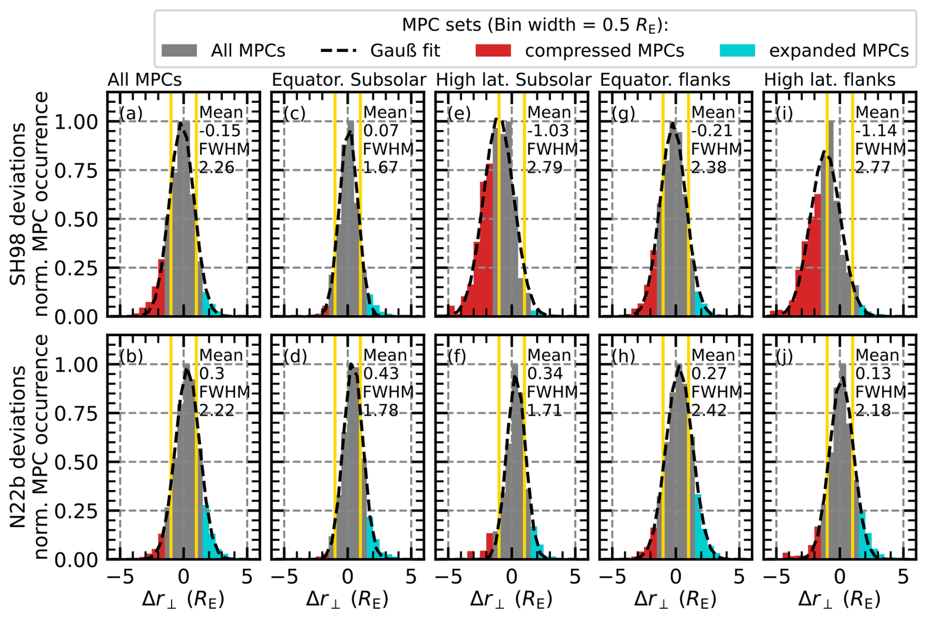
Figure 2 Distributions of Δr_⟂ between the observations in the combined data sets and the prediction of the SH98 model in panel (a) and the prediction of the N22b model in panel (b). The distributions from (a) and (b) are split into subsets: (c) and (d) show the distributions for the subsolar magnetopause, (e) and (f) show the high-latitude MP in the noon sector, (g) and (h) show the flank MP observations in the equatorial plane, and (i) and (j) show the flank MP observations in the high latitudes. The yellow lines represent the 1 R_E uncertainty of the MP models reported by Case and Wild (2013) and Staples et al. (2020). The red- and cyan-coloured regions of the histograms are the MPCs that clearly deviate from the selected model in the data set (see text for details). The dashed black lines represent a Gaussian fit to the histograms, with the mean and median and the full width at half maximum (FWHM) of the fits also shown. The normalization of the distribution is done, firstly, by dividing by the spacecraft dwell time in each bin and, secondly, by scaling the distribution to the maximum occurrence rate.

Panels (a) and (b) of Fig. 2 show the distributions of Δr_⟂, the deviation between the observation and the models being considered. In order to eliminate any orbital bias in the histogram, we used the dwell time of the spacecraft in each bin for normalization. Here, the dwell time should be seen as the time during which the spacecraft are within the different bins (i.e. between certain ranges of model deviations) and can potentially observe an MPC with the associated model deviation. The normalization therefore provides a more realistic distribution of the occurrence of MPC deviations as MPCs found in regions frequently visited by the spacecraft show reduced importance.

Both distributions show a similar width according to a Gaussian fit we applied, which gives a value of full width at half maximum (FWHM) of 2.26 (2.22) R_E for the SH98 (N22b) model. Thus, we can identify quite a few crossings with $\left|\mathrm{\Delta }{r}_{⟂}\right|>\mathrm{1.5}{R}_{\mathrm{E}}$ where the observed location differs from the predicted one in both distributions (cyan- and red-coloured events). For the SH98 model, 14.5 % of the events are either overestimated or underestimated MPCs, and for the N22b model, 12.7 % are misrepresented MPCs. However, an important difference between the distributions is the mean and/or median of the fit: −0.15 R_E for the SH98 model and 0.3 R_E for the N22b model. This leads to the fact that the N22b model, when compared to the SH98 distribution, has significantly more underestimated MPCs.

Figure 2c–j show the regionally separated distributions of Δr_⟂. There are a few things worth noting. In both figures, it is clear that the distributions for the flank regions (panels g–j) are broader than the distributions for the two subsolar regions (panels c–f). In general, the distribution for the equatorial subsolar region with an FWHM value of 1.67 (1.78) R_E, considering the SH98 (N22b) model, shows the narrowest distribution, with mostly underestimated MPCs outside the error bounds of the model prediction. The distributions for the deviation from the SH98 model are shifted to negative deviations in the high-latitude regions (see Fig. 2e and i), resulting in a lot of overestimated MPCs in these subsets. Since the SH98 model does not include a cusp indentation, the encounter of the cusp in the high-latitude regions causes a bias towards overestimated MPCs in the Δr_⟂ distribution, which is clearly visible here and was reported by Grimmich et al. (2024b) for the Cluster data set used here. The N22b model includes an indentation term for the cusp, and we can see in Fig. 2f and j that this results in a narrower distribution, with drastically fewer overestimated MPCs. However, we can also see the shift towards positive deviations of Δr_⟂ in all regions for the N22b model, which, of course, also reduces the number of observed overestimated MPCs in the high latitudes.

Since we calculate an estimate for ϑ_B,n of the bow shock for each MPC, we can show here which bow shock configuration (quasi-parallel for ${\mathit{\vartheta }}_{B,n}<\mathrm{45}$, quasi-perpendicular for ${\mathit{\vartheta }}_{B,n}>\mathrm{45}$) is favourable for the occurrence of misrepresented MPCs. We identify favourable conditions, similarly to the favourable solar-wind conditions identified by Grimmich et al. (2023a, 2024b) for the THEMIS and Cluster data sets. We compare the occurrence of ϑ_B,n associated with overestimated and underestimated MPCs with the total occurrence of different bow shock configurations over the course of the three missions.

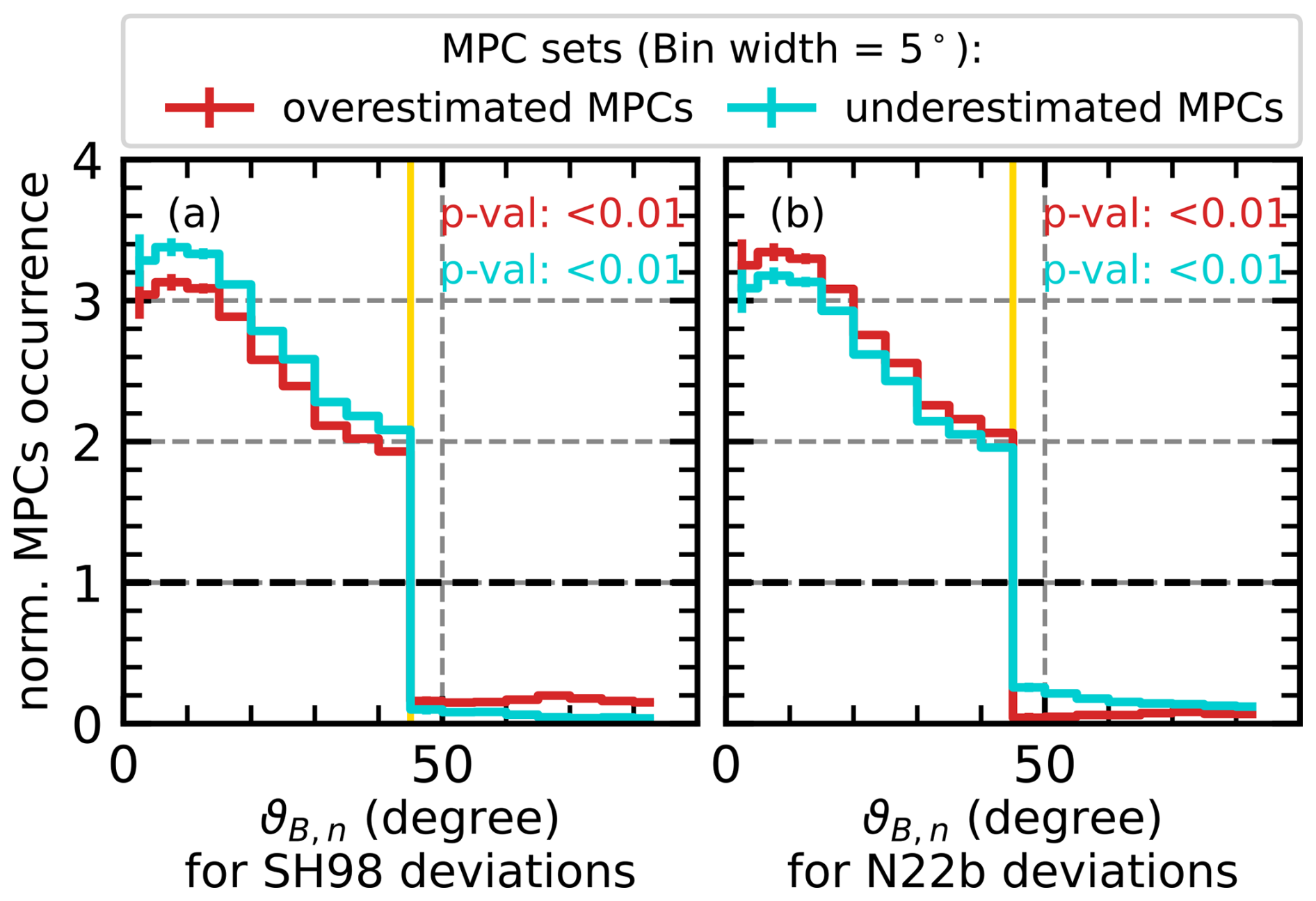
Figure 3 The ϑ_B,n distributions for the overestimated and underestimated MPCs misrepresented in the SH98 (a) and N22b (b) model are shown in red and cyan, respectively. The distributions are normalized by dividing by the total number of different ϑ_B,n values. A value of 1 in the plots (dashed black line) would therefore indicate that the occurrence of misrepresented MPCs is identical to the total occurrence, while values greater than 1 indicate that misrepresented MPCs occur more frequently under these conditions. The yellow lines mark the boundary between the quasi-parallel and the quasi-perpendicular foreshock condition associated with ϑ_B,n. In addition, we show in each panel for the subsets the p value that results from a Mann–Whitney U test: values less than 0.05, which are shown in the case here, indicate statistically significant deviations from the reference distribution.

Figure 3 again compares the results for the two different models. The distributions of ϑ_B,n associated with the outlying MPCs have been normalized by dividing these distributions by the reference distribution, which includes all times when a given ϑ_B,n value is observed and is not restricted to times when MPCs are observed. Thus, a value of 1 in the plots indicates that the overall distribution and that associated with the overestimated or underestimated MPCs are the same, and we can identify favourable conditions by looking for areas where we see values above 1.

In order to be sure that the observed deviations are statistically significant and not due to chance, we performed a Mann–Whitney U test. This test is a generalization of Student's t test for non-normal distributions like ours and is used to analyse the differences between two independent samples with similar shapes.

The null hypothesis of the test is always that there are no significant differences between the samples, which, in our case, would mean that the distribution of deviant events is the same as the reference distribution. To reject or accept the null hypothesis, a rank is assigned to each observation. The ranks are then summed for each group. The test statistic U value is calculated from these rank sums for each distribution, and the smaller of the U values is used for hypothesis testing. If the calculated U value is less than the critical value from the Mann–Whitney distribution (based on sample sizes), the null hypothesis is rejected, indicating a significant difference between the two groups. In our case, the probability value from the test statistic must be smaller than 0.05 (see Mann and Whitney, 1947, for more details).

Here, the test results in probability values well below 0.01; thus, the distribution of ϑ_B,n associated with deviant events is significantly different from the overall distribution of ϑ_B,n, which assures the seen favourable conditions for deviant events.

We can clearly see that, for both models and for the occurrence of both overestimated and underestimated MPCs, ${\mathit{\vartheta }}_{B,n}<\mathrm{45}$° constitutes favourable conditions. Thus, MPCs behind the quasi-parallel bow shock where foreshock has developed tend to deviate more from the MP observation. In addition, we can extract from our data set that 42 % (38 %) of the MPCs deviating from the SH98 (N22b) model predictions are associated with the quasi-parallel bow shock conditions and likely foreshock activity and that 19 % (15 %) of the observed MPCs associated with ${\mathit{\vartheta }}_{B,n}<\mathrm{45}$ and q>0 deviate from the SH98 (N22b) model prediction. Considering the fact that ${\mathit{\vartheta }}_{B,n}<\mathrm{60}$° is sometimes also used to define the boundary of the active foreshock region (Wilson, 2016; Karlsson et al., 2021), about 54 % of the misrepresented MPCs might be associated with foreshock activity.

Since we know that, under quasi-parallel conditions, the MP can be highly disturbed and the occurrence of misrepresented MPCs in both directions (overestimated and underestimated MPCs) is likely, we look again at the Δr_⟂ distribution in different regions to see if the conditions in one region have a particular influence. Figure 4 shows, for the SH98 and N22b models, the comparison of the distributions of Δr_⟂ associated with quasi-parallel and quasi-perpendicular conditions for all MPCs and in the four MP regions defined above.

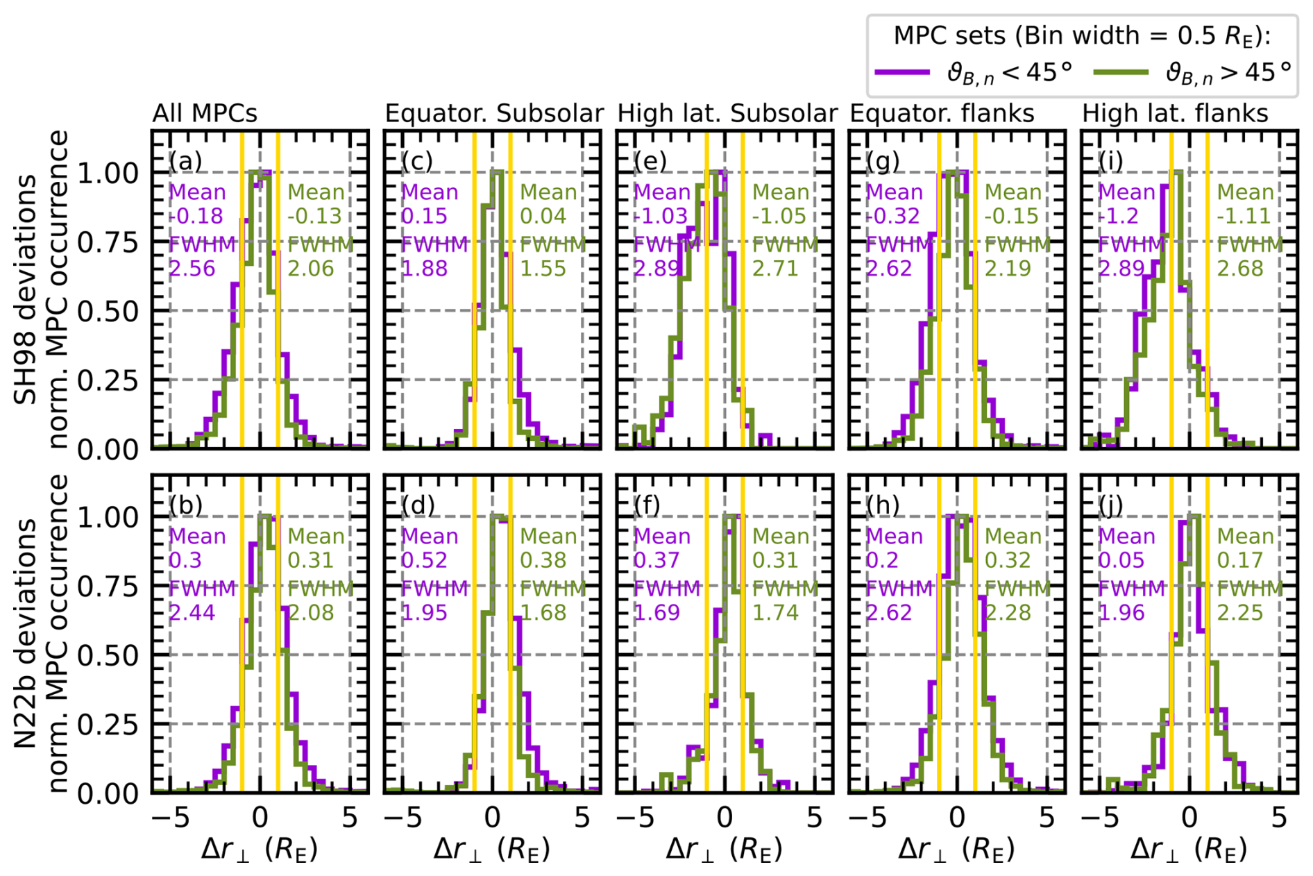
Figure 4 Comparison of Δr_⟂ distributions of MPCs associated with different ϑ_B,n in different magnetospheric regions. As in Fig. 2, panels (a) and (b) show the distributions that include all of the MPC observations, (c) and (d) show the distributions for the subsolar magnetopause, (e) and (f) show the high-latitude MP in the noon sector, (g) and (h) show the flank MP observation in the equatorial plane, and (i) and (j) show the flank MP observation in the high latitudes. The violet distributions belong to MPCs associated with ${\mathit{\vartheta }}_{B,n}<\mathrm{45}$°, observed behind a quasi-parallel foreshock region, while the green distributions belong to MPCs associated with ${\mathit{\vartheta }}_{B,n}>\mathrm{45}$°. For each distribution, the mean and/or median and full width at half maximum (FWHM) values of an associated Gaussian fit are also displayed, and the yellow lines mark the reported 1 R_E uncertainty of the MP model.

Figure 4a and b show a visible effect of the presence of the foreshock region on the general Δr_⟂ distributions, with negligible shifts in the mean and/or median but noticeable broadening of the distributions. Specifically, the bow shock condition seems to have the largest effect on the subsolar region. This is somewhat to be expected as the MP in this case is immediately downstream of the foreshock, which is not the case at higher latitudes. In Fig. 4c and d, we notice a shift towards larger positive deviations from the model predictions if the MPCs are associated with quasi-parallel conditions; the mean and/or median value of the Gaussian fit for the SH98 (N22b) model distribution shifts from 0.04 (0.38) R_E to 0.15 (0.52) R_E when the MPCs are associated with quasi-parallel conditions. We can also see that the quasi-parallel distribution is significantly wider compared to the quasi-perpendicular distribution in the subsolar region (cf. FWHM values in panel c), indicating an increased variability of the MP location, e.g. due to more frequent motion.

Although we see a slight broadening of the Δr_⟂ distribution associated with low ϑ_B,n values for both models in the flank and high-latitude regions (panels e to j), accompanied by a mostly negligible shift in the distribution, the influence is not as pronounced. At the flanks, the quasi-parallel distributions shift by about 0.1 to 0.15 R_E towards negative deviations, while, at the high-latitude subsolar MP, the shift is about 0.02 to 0.06 R_E towards positive deviations.

Since general asymmetries between the dawn and dusk magnetosphere have been reported, especially with respect to the waves and undulations of the MP surface but also in internal magnetospheric properties such as plasma density (e.g. Russell et al., 1997; Nykyri, 2013; Walsh et al., 2014; Archer et al., 2015a; Henry et al., 2017), assessing both flanks in one subset might obscure different effects that are important on only one flank. We therefore decided to separate our flank subsets again into dawn and dusk. This will also give us more information on how well the two models have predicted the magnetopause at different locations, which may help to further improve one of them.

So if we look at the dawn and dusk flanks separately, we find a general asymmetry in the Δr_⟂ distributions (see Fig. 5): in the equatorial plane (panels a–d), the distributions on the dusk flank are narrower, with a mean shifted towards positive deviations, whereas the distributions on the dawn flank are wider, with a mean and/or median shifted towards negative deviations. While at high latitudes (panels e–h) the shift of the means and/or medians between dawn (more towards negative deviations) and dusk (more towards positive deviations) is the same as at the equatorial latitudes, the width of the distributions is different, with wider distributions at high-latitude dusk flanks and narrower distributions at high-latitude dawn flanks. The shifts in the means and/or medians indicate that, on average, the models tend to under-predict the location of the MP at dusk and over-predict the location of the MP at dawn.

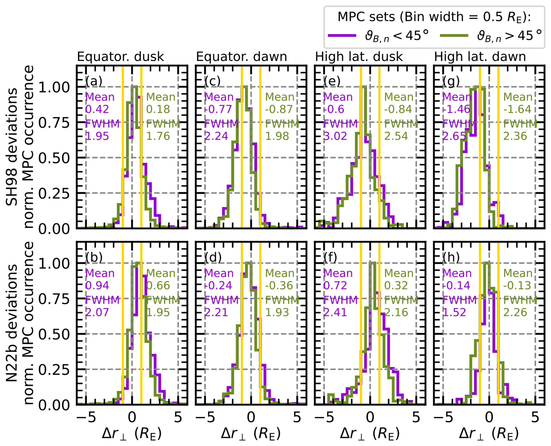
Figure 5 Comparison of Δr_⟂ distributions of MPCs associated with different ϑ_B,n on the dawn and dusk flanks. Panels (a) and (b) show the distributions for the equatorial dusk flank MPC observations, (c) and (d) show the distributions for the equatorial dawn flank, (e) and (f) show the high-latitude MP at the dusk flank, and (g) and (h) show the high-latitude MP at the dawn flank. The violet distributions similar to Fig. 4 belong to MPCs associated with ${\mathit{\vartheta }}_{B,n}<\mathrm{45}$°, while the green distributions belong to MPCs associated with ${\mathit{\vartheta }}_{B,n}>\mathrm{45}$°. For each distribution, the mean and/or median and the full width at half maximum (FWHM) of an associated Gaussian fit are also shown, and the yellow lines mark the reported 1 R_E uncertainty of the MP model.

In addition to these general observations on the dawn and dusk flanks, we can also see a similar widening of the distribution associated with foreshock activity (i.e. for ${\mathit{\vartheta }}_{B,n}<\mathrm{45}$), as in the other regions shown in Fig. 4. In the equatorial plane, the distributions on the dawn flanks widen by almost one-third more than the distribution on the dusk flank when foreshock activity leads to more frequent deviations from model predictions due to the more turbulent motion of the MP surface behind a quasi-parallel bow shock.

We also find something similar to the effect seen in the subsolar region as the separation in the dawn and dusk flank crossings shows a shift of the distributions towards positive deviations (i.e. towards an underestimation of MP locations) on both flanks. This is in contrast to Fig. 4g and h, where the distributions appear to be shifted towards negative deviations (i.e. towards an overestimation of MP locations) under quasi-parallel conditions. The previously observed shift towards negative values is most likely a result of the asymmetry between the two flanks as the dawn flank crossings are generally shifted towards these values and also have a stronger difference between quasi-parallel and quasi-perpendicular conditions.

We would like to point out that this asymmetry could be a result of the fitting of the models used. If the models were fitted to non-aberrated coordinates then applying them to aberrated coordinates would cause the asymmetry we see. However, to our knowledge, both models used the aberrated coordinates to fit their respective models. Therefore, application to our data should not result in the asymmetry seen. This suggests that the asymmetry most likely has a more physical explanation, such as, for example, the more frequent occurrence of KHIs and the subsequent waves at the dawn flank MP (e.g. Kavosi and Raeder, 2015; Nykyri et al., 2017; Henry et al., 2017).

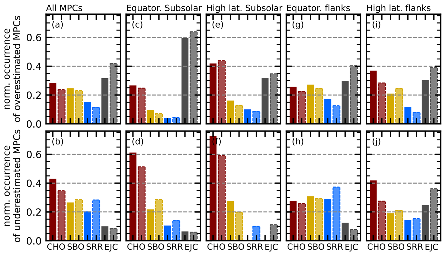
Figure 6 Comparison of the occurrence of overestimated MPCs (a, c, e, g, i) and underestimated MPCs (b, d, f, h, j) misrepresented in the SH98 and the N22b models for different solar-wind plasma conditions. The distribution associated with the SH98 model is shown as solid bars, while the distributions associated with the N22b model are shown as slightly transparent bars with dashed edges. The solar-wind conditions are grouped according to the classification scheme of Xu and Borovsky (2015), with different colours corresponding to different solar-wind types: red for coronal-hole origin (CHO), yellow for streamer belt origin (SBO), blue for sector reversal region (SRR), and grey for ejecta (EJC). Each bin is normalized by dividing the count rate of MPCs during a particular solar-wind type by the count rate of that solar-wind type in the OMNI data during the observation period and then scaling for each model in such a way that the combined occurrence of all four types is equal to 1 in each panel. Panels (a) and (b) show the combined MPC data set events, panels (c) and (d) show the MPC events observed in each subsolar region, panels (e) and (f) show the events observed in high-latitude subsolar regions, panels (g) and (h) show the events observed in equatorial flank regions, and panels (i) and (h) show the events observed in high-latitude flank regions.

Besides the influence of the bow shock configuration, which seems to correlate well with some of the observed deviations from model predictions, we also want to better determine the solar-wind conditions responsible for the deviations. Since we have associated each MPC with a corresponding solar-wind plasma class, we can investigate the occurrence of misrepresented MPCs for a combination of solar-wind parameters (instead of the single-parameter influence investigated by Grimmich et al., 2023a, 2024b).

In Fig. 6, we show the normalized occurrence of overestimated and underestimated MPCs during the different solar-wind conditions based on the Xu and Borovsky (2015) scheme in the four different magnetopause regions for both models. Normalization was performed by dividing each number of occurrences of a particular class associated with an MPC by the total number of occurrences of that class in the OMNI data set between 2001 and 2024 before scaling the distribution in each panel for each model in such a way that the combined occurrence of all four types is equal to 1. While the relative abundance of classes for each panel is not affected by normalization, comparisons between panels must be made with caution as the scaling for better visibility may distort the view of the importance of classes in different panels.

The figure allows a direct comparison between the two models and mainly shows the agreement between the two, revealing the most important classes of solar-wind present when overestimated and underestimated MPCs occur. In order to provide further information on the solar-wind conditions responsible for the occurrence of deviant MPCs, the results of the separation of the four plasma classes according to the IMF direction are shown in Tables 3 and 4.

Table 3 Comparison of the relative occurrence rates of overestimated MPCs deviating from the SH98 and N22b models for different solar-wind plasma conditions. The solar-wind conditions are grouped according to the classification scheme of Xu and Borovsky (2015): coronal-hole origin (CHO), streamer belt origin (SBO), sector reversal region (SRR), and ejecta (EJC). Each solar-wind type is further divided into three subcategories corresponding to the IMF direction: quasi-radial IMF, northward IMF, and southward IMF. The maximum occurrence rates for a given direction in each row are highlighted in bold. The values for the general solar-wind classes are taken from Fig. 6, while the IMF direction indicates which of the directions is the most common relative to the occurrence of the type.

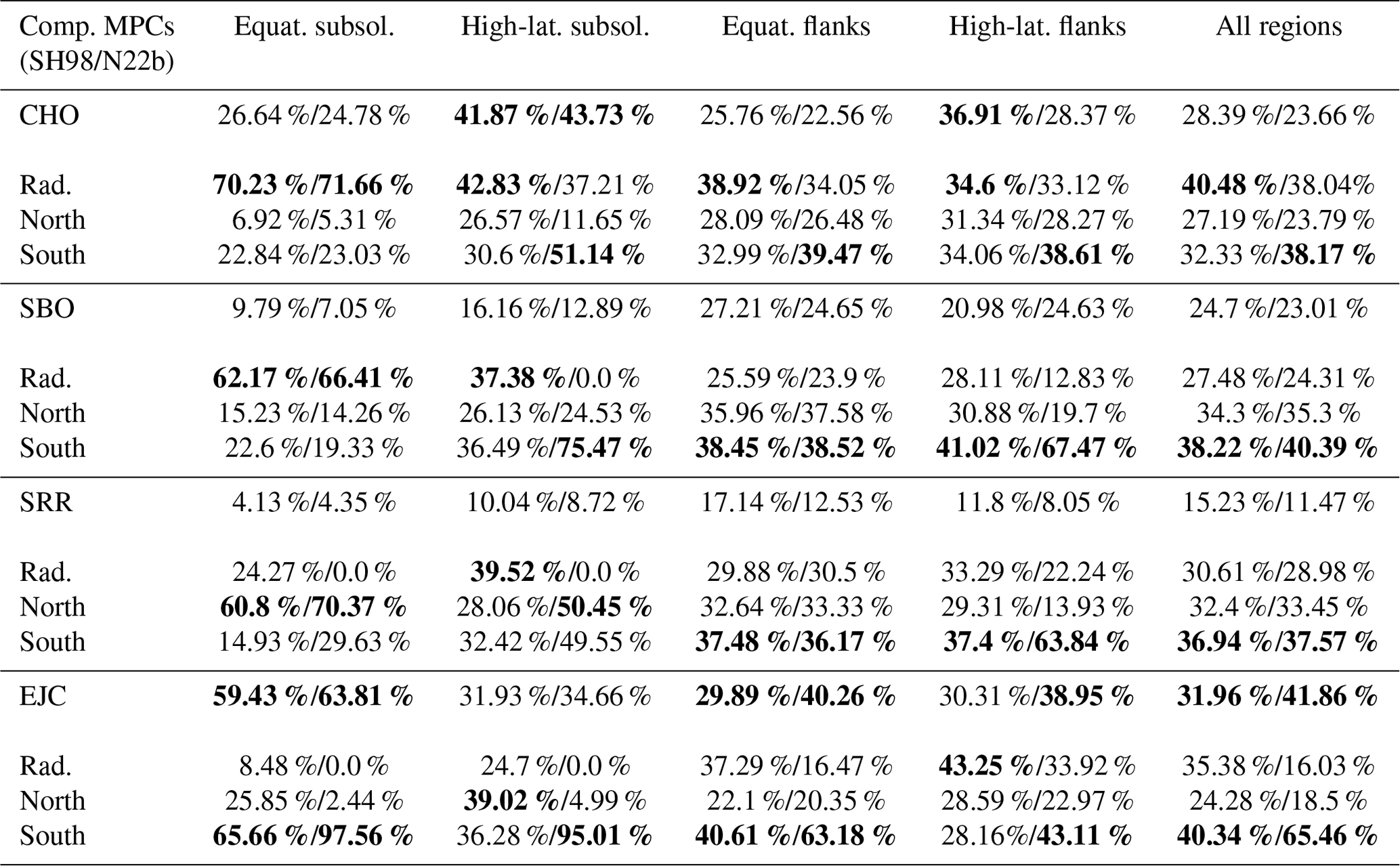
Table 4 Comparison of the relative occurrence rates of underestimated MPCs deviating from the SH98 and N22b models for different solar-wind plasma conditions. The solar-wind conditions are grouped according to the classification scheme of Xu and Borovsky (2015): coronal-hole origin (CHO), streamer belt origin (SBO), sector reversal region (SRR), and ejecta (EJC). Each solar-wind type is further divided into three subcategories corresponding to the IMF direction: quasi-radial IMF, northward IMF, and southward IMF. The maximum occurrence rates for a given direction in each row are highlighted in bold. The values for the general solar-wind classes are taken from Fig. 6, while the IMF direction indicates which of the directions is the most common relative to the occurrence of the type.

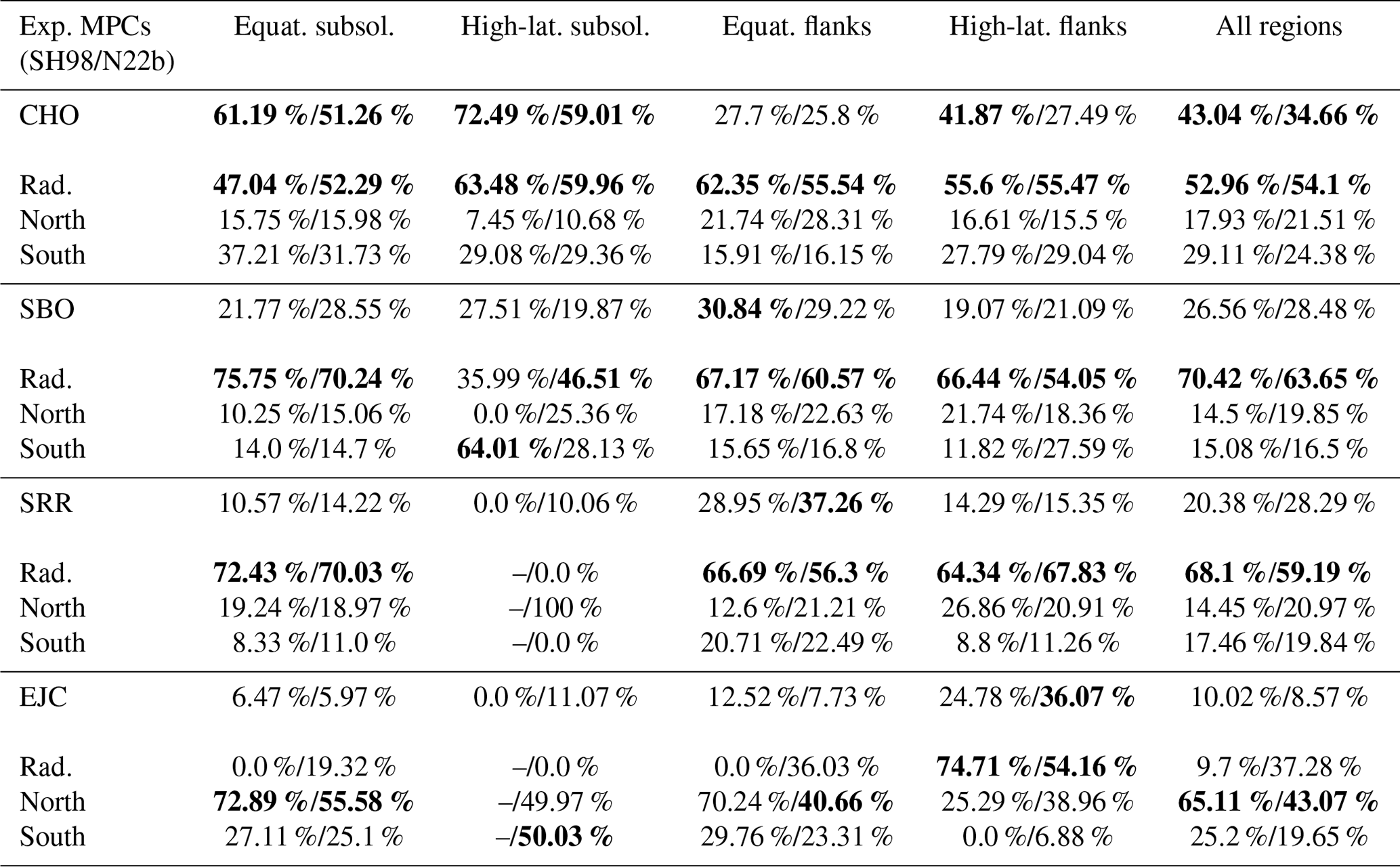
We see some clear dependencies for the occurrence of misrepresented MPCs (more or less independent of the model used to determine these MPCs): overestimated MPCs are clearly common for southward-IMF orientations, with only EJC plasma being quite prominent. However, we also see that SBO and CHO plasma are similarly abundant when overestimated MPCs are observed (see Table 3). Interestingly, the radial IMF seems to play a role, especially in the high-latitude regions in the CHO plasma, according to the SH98 deviations (Table 3). Underestimated MPCs occur most frequently under any radial-IMF direction and most frequently during the CHO solar wind (see Fig. 6 and Table 4). Although CHO dominates, SBO and SRR plasma become more important for underestimated MPCs on the flank (panels h and j), while, seemingly, EJC solar wind plays a role almost only for high-latitude flank crossings (panel j).

It should be noted that there are obvious differences between the results associated with the SH98 and N22b models (e.g. in panels i and j). However, these differences can easily be attributed to the lack of data for overestimated and underestimated MPCs associated with one or the other model in certain magnetospheric regions (see Table 2).

Similarly to the Δr_⟂ distributions, we want to separate the distribution of the occurrence of misrepresented MPCs associated with different solar-wind classes into MPCs behind a quasi-parallel and a quasi-perpendicular bow shock using ϑ_B,n. Therefore, Fig. 7 shows the occurrence under the solar-wind classes for MPCs with ${\mathit{\vartheta }}_{B,n}<\mathrm{45}$° and ${\mathit{\vartheta }}_{B,n}>\mathrm{45}$°; the overestimated and underestimated MPCs are selected with the SH98 and N22b models, respectively. For both models, we can again see similar characteristics for the occurrence of misrepresented MPCs.

Figure 7 Comparison of the occurrence of overestimated MPCs (top panels) and underestimated MPCs (bottom panels) misrepresented in the SH98 and N22b MP models for different solar-wind plasma conditions, similarly to Fig. 6. Here the solar-wind classes are also separated for the IMF orientation with quasi-radial IMF (r.), northward IMF (n.), and southward IMF (s.). The occurrence of misrepresented MPCs associated with ${\mathit{\vartheta }}_{B,n}<\mathrm{45}$° (panels (a) and (b) for SH98 deviations and panels (e) and (f) for N22b deviations) is compared to the occurrence of misrepresented MPCs associated with ${\mathit{\vartheta }}_{B,n}>\mathrm{45}$° (panels (c) and (d) for SH98 deviations and panels (g) and (h) for N22b deviations).

We can see more clearly that, for the overestimated MPCs (top panels of Fig. 7), the southward-IMF and EJC plasma is responsible for deviations behind quasi-perpendicular bow shock conditions, while radial-IMF conditions within all plasma types occur often for the events behind the quasi-parallel bow shock. Furthermore, CHO plasma appears to be more important for the quasi-parallel conditions than for the quasi-perpendicular conditions. It also seems that SBO and CHO plasma types are similarly abundant only for overestimated MPCs behind the quasi-perpendicular bow shock (see panels e and g).

For the underestimated MPCs (bottom panels of Fig. 7), we see the importance of the CHO plasma for the occurrence independent of the bow shock conditions. We also see more clearly that radial-IMF conditions could be mainly responsible for the underestimated MPCs behind the quasi-parallel bow shock (see panels b and d). Overall, we can see that, in 50 % (49 %) of the cases, we encounter underestimated MPCs that deviate from the SH98 (N22b) model behind a quasi-parallel bow shock, and the IMF orientation is quasi-radial. Otherwise, it is interesting to note that southward-IMF conditions (mostly in CHO plasma) seem to be quite common for underestimated MPCs behind the quasi-perpendicular bow shock for the SH98 deviations (see panel f). According to panel (h), the SRR plasma and the northward IMF occur simultaneously with the deviation from the N22b model predictions, which is in stark contrast to the SH98 results. This may be an effect of the general underestimation of MP location in the N22b model, resulting in more underestimated MPCs deviating from this model compared to the SH98 model.

4 Discussion

Our investigation aimed to better identify the reasons why the spacecraft-observed position of the MP surface can differ quite substantially from the empirical model predictions. We build on the results of Grimmich et al. (2023a, 2024b) and combine three large data sets of dayside MPCs, including data from the Cluster, THEMIS, and MMS missions, to comprehensively examine the dayside MP over a wide range of longitudes and latitudes. However, the different sizes of the data sets and the orbital inclinations of the missions have the disadvantage that not all magnetospheric regions are covered equally, as can be seen in Table 2, which might affect occurrence rates. Nevertheless, the different orbits are also beneficial as the bias of uneven coverage of annual solar-wind conditions due to variations in spacecraft apogees, causing misinterpretation of occurrence rates, as reported by Vuorinen et al. (2023), should be substantially reduced by combining the different data sets. Thus, our results from the combined data set should be better overall at revealing the influences of the solar wind on the position of the MP than previous studies using only a single mission data set.

However, another orbital bias of concern could be due to the apogee of the spacecraft being lower than the average position of the boundary. As a result, spacecraft can only sample the MP at certain distances, which may belong to the innermost transient excursions or intervals of high solar-wind pressure (e.g. Němeček et al., 2020). This is a particular problem in the flanks near the terminator, which has a nominal MP location of about 14.5 R_E, while the spacecraft of, for example, THEMIS have apogees of about 13.2–13.7 R_E. This can obviously lead to more frequent observations of overestimated MPCs and very few observations of underestimated MPCs at the flanks and could explain the shift in the distribution towards negative deviations from the MP models. Furthermore, this bias could also be a factor in the difference between the dawn and dusk flanks that we highlighted in Fig. 5. Therefore, our results regarding the magnetic flanks must be treated with caution and should be further investigated in the future.

Another point that helps to generalize and understand the occurrence of misrepresented MPCs is that we have chosen to use two different empirical MP models to identify deviant boundary-crossing events. The Shue et al. (1997, 1998) model is one of the simpler models, and, despite its deficiencies, it is widely used in the community (e.g. in the previous studies of Grimmich et al., 2023a, 2024b) to represent the basic behaviour of the MP surface and was therefore included here. The Nguyen et al. (2022a, b) model is claimed to be one of the most accurate empirical models, including all kinds of observed asymmetries and also the important cusp indentations in the high-latitude regions for MP surface modelling. Given that the cusp indentation term, adapted from Liu et al. (2015), used in the N22b model is more accurate than the one used in the Lin et al. (2010) model (Nguyen et al., 2022a), we have chosen the N22b model over the Lin et al. (2010) model for the comparison in this study. To our knowledge, this model has not been validated on independent data, which is another reason why we have decided to include it here to see if it is, indeed, more accurate. Other models, such as the Petrinec and Russell (1996) model, were not considered here because they focus on the nightside, whereas our study is limited to the dayside.

The comparison of the two models has allowed us to see if the occurrence of misrepresented MPCs is model dependent or if there is a lack of fundamental physical understanding in the models. Despite the fact that the two MP models used were developed based on very different data sources and have different input parameters, the occurrence of model deviations and the associated conditions that may be responsible are very similar. Indeed, this seems to indicate systematic biases due to uncaptured physics in the models, although, since the MP is almost always in motion, some scatter is to be expected and will remain even if the models can be improved by our results.

We also want to address the problem of ignoring the time history of the solar wind. There are processes, such as the erosion of the MP towards a quasi-stationary endpoint closer to Earth, that occur over a longer time frame rather than instantaneously, as implemented in the average models used. Some of our deviant events may be due to such an effect as the solar wind used for the modelling already suggests a different location towards which the observed MP is actually still moving.

As shown in Fig. 2a and b, the distribution of the model deviation Δr_⟂ has an almost identical width of 2.26 R_E and 2.22 R_E, and for both models, 12 % to 14 % of the crossings are misrepresented MPCs, indicating that their general occurrence seems to be model independent. Since several studies (e.g. Šafránková et al., 2002; Case and Wild, 2013; Nguyen et al., 2022b; Aghabozorgi Nafchi et al., 2024) point out similar uncertainties inherent in the empirical modelling (in part due to the constant motion around an average location of the MP), this is not surprising. The obvious difference in the distribution of misrepresented MPCs between the two models (with the SH98 model, we get more overestimated MPCs, while the N22b model identifies more underestimated MPCs; see Table 2) probably stems from two sources (in addition to the aforementioned orbital biases): (1) the cusp encounters in the high-latitude crossings observed by Cluster lead to a bias towards overestimated MPCs for the non-indented SH98 model (see, for example, Boardsen et al., 2000; Šafránková et al., 2002, 2005; Grimmich et al., 2024b). (2) In general, the N22b model seems to underestimate the location of the MP surface for about 0.3 R_E and therefore has a clear bias towards extended MPCs.

There could be a number of reasons for this. One possibility is that the functional form – and, in particular, the dependence of the IMF on the stand-off distance – is not appropriately chosen in the N22b model. As mentioned above, the effect of the IMF B_z component on the stand-off distance is visibly weaker compared to that of the SH98 model. This results in a much less pronounced expansion of the dayside MP for the northward IMF and a weaker MP erosion for the strong southward IMF. As a result, the comparative distribution between observed and modelled MP locations for the N22b model may be visibly shifted relative to the SH98 model distributions, as seen in our plots. Another reason why the N22b model underestimates the MP location could be that the fitting of this model was influenced by the orbital apogee bias. If only the innermost crossings further away from the average MP location were included in the fitting procedure, this would result in a model trained to always predict distances closer to Earth.

Overall, the SH98 model (despite the obvious bias from the cusp indentations and the problem of apogee coverage) is better at predicting average MP location than the N22b model. Nevertheless, the effects on the misrepresented MPCs are visible in both models, and in the following, we will only point out and discuss what is visible for both models.

Although, for example, Aghabozorgi Nafchi et al. (2024) suggest that the deviations between observations and models are primarily due to inaccurate propagation of solar-wind parameters from the L1 point (measurement point of the OMNI data set) to Earth, we may have found other but also adjacent possible explanations in this study. As Figs. 3, 4, and 5 show, MPCs associated with quasi-parallel bow shock conditions (i.e. ${\mathit{\vartheta }}_{B,n}<\mathrm{45}$) are quite often deviant crossing events. This suggests that the development of the foreshock region is an important factor in the occurrence of these events. The foreshock region strongly modifies the upstream solar-wind conditions affecting the magnetosphere due to its turbulence but also due to the occurrence of unpredictable transients (Fairfield et al., 1990; Russell et al., 1997; Plaschke et al., 2013; Walsh et al., 2019; Zhang et al., 2022). This explains the discrepancies nicely as, due to the foreshock modifications, the inputs to the models are not the conditions in the vicinity of the MP that determine the boundary position.

Here, we propose that about 40 %–60 % (depending on the limit of ϑ_B,n chosen for the foreshock activity) of the deviant cases in the combined data set are associated with foreshock activity and are therefore likely to be explained by the foreshock influence. This influence seems to be strongest for the subsolar MP, and we can estimate from comparing the means in Fig. 4c and d that the MP is, on average, 0.12 R_E more sunward for these MPCs associated with foreshock activity. In addition, for the equatorial flanks (Fig. 5a–d), we see an asymmetry between dawn and dusk: the MP under foreshock influences is, on average, about 0.26 R_E more anti-earthward on the dusk flank and, on average, about 0.11 R_E more anti-earthward on the dawn flank. Furthermore, the MP clearly shows more motion on the dawn flank under foreshock influence as the distribution of model deviations is wider compared to on the dusk flank.

However, not all MPCs associated with the quasi-parallel bow shock conditions are affected by the foreshock in an extreme way; only 17 % of the crossings behind a foreshock can be identified as misrepresented MPCs, while, in the other case, the model predictions seem to agree with the observations, and the foreshock might cause only a smaller-amplitude motion around the mean location. Therefore, the presence of the foreshock does not guarantee the occurrence of a deviant MPC.

It is also important to note again that our ϑ_B,n estimate may not be the angle at the bow shock, which is upstream of the MP undulation. The shocked solar-wind plasma propagates through the magnetosheath along streamlines (e.g. Russell et al., 1983; Luhmann et al., 1986), and, depending on the orientation of the IMF, this may lead to regions of the MP being affected by the quasi-parallel shock, although our estimate indicates a quasi-perpendicular shock (or vice versa). We tried to validate our estimates of the foreshock state using a second method by Petrinec et al. (2022), which largely agrees with our initial guesses. Thus, the effect of a misclassified upstream bow shock configuration may not be severe.

In addition, Kavosi and Raeder (2015) have shown in a statistical study that KHI forms more or less independently of the IMF cone angle and, therefore, most likely also forms from the foreshock activity. Since large KHI waves can be responsible for the observation of misrepresented MPCs (as discussed in, for example, Grimmich et al., 2023a), the misrepresented MPCs most likely to be influenced by the foreshock may, to some extent, actually be caused by KHI. However, it is still unknown to what extent the convected foreshock oscillation could influence the development of the KHI. Thus, it is not easy to determine which of these two is the source of the deviating MPC observations, and future studies should aim to separate this effect and possibly assess to what extent the foreshock triggers the KHI and to what extent the KHI occurs independently.

By looking at the influences of the solar-wind classes introduced by Xu and Borovsky (2015) on the occurrence of deviating MPCs, we can potentially identify and differentiate additional sources of deviations from the models. In Figs. 6 and 7, we can see which solar-wind parameter combinations are most likely to be present during the encounter with misrepresented MPCs.

A CHO plasma, described by high solar-wind speeds and temperatures with low ion densities and intermediate IMF magnitudes (compared to the average parameter values from the OMNI data), is most often present when underestimated MPCs occur. Consistently with this finding, high solar-wind speeds (independent from other parameters) have previously been reported to be favourable for the onset of (large) sunward MP deformation (Grimmich et al., 2023a, 2024b; Guo et al., 2024). This result now allows us to estimate the magnitude of other solar-wind parameters that typically occur at high solar-wind speeds as well.

Another point often found in the literature is the expansion of the MP under quasi-radial-IMF conditions (Merka et al., 2003; Suvorova et al., 2010; Samsonov et al., 2012; Park et al., 2016; Grygorov et al., 2017; Guo et al., 2024), and so this orientation is naturally often associated with underestimated MPCs, which is also visible in our findings. In addition, our results show that the underestimated MPCs that occur during quasi-radial-IMF conditions are associated with quasi-parallel bow shock conditions significantly more often. Since, under radial-IMF conditions, the foreshock develops upstream of the subsolar bow shock to where the IMF is tangent to the bow shock surface – as a result of which, most of the dayside magnetosphere would be behind a quasi-parallel bow shock – this observation is not surprising.

In combination with the likely presence of CHO plasma simultaneously with quasi-radial IMF, our findings further emphasize that, besides the “normal” turbulence influencing the MP, foreshock transients might often be responsible for the misrepresented MPCs. These transients occur more frequently in the foreshock under exactly these conditions (Chu et al., 2017; Vu et al., 2022; Zhang et al., 2022; Xirogiannopoulou et al., 2024), and several studies have already shown that the very different plasma parameters in the core of these transients can significantly deform the MP towards the Sun (e.g. Sibeck et al., 1999; Turner et al., 2011; Archer et al., 2015b; Grimmich et al., 2024c). It is also worth noting that the foreshock developed in the CHO plasma should be further investigated. This could explain exactly why the MP appears to move globally outwards under radial IMF, which is most likely accompanied by CHO plasma. The composition of this plasma group could therefore be the dominant factor missing in the explanation. However, a recent study by Lee et al. (2024) showed that, for “fast” solar wind, the IMF more often becomes quasi-radial-IMF, and discontinuities in the solar wind are more often oriented in a direction where they can produce larger foreshock transients when hitting the Earth's bow shock. Thus, this favourable orientation and the growth of the transients under the quasi-radial-IMF conditions may be the reason that we can observe the transient-misrepresented magnetopause locations caused.

Contrarily to the finding of Grimmich et al. (2023a), which suggest that high Alfvén Mach numbers and solar-wind plasma β are also important for the occurrence of underestimated MPCs, we find that the SRR plasma described by these conditions is less important and actually only relevant together with the radial IMF, which is likely to be the dominant effect for the occurrence of misrepresented MPCs. This shows that our classification of the solar wind and looking at the influences from combined data sets help to distinguish the more important mechanisms.

For the underestimated MPCs associated with quasi-perpendicular bow shock conditions, which, as a result, are probably not caused by the foreshock modification, we see that, for the SH98 model deviations, southward CHO plasma is mostly present during the observations. Since we see that this occurrence of southward CHO plasma is associated with the subsolar region at low and high latitudes (Table 4), one explanation for the underestimated MPCs could be that large flux transfer events (Elphic, 1995; Dorelli and Bhattacharjee, 2009; Fear et al., 2017) resulting from ongoing reconnection at the MP nose under southward IMF lead to displacements of the MP surface. However, these results are largely due to the high-latitude underestimated MPCs, which are rather sparse in our data set compared to the other regions. Therefore, there is no guarantee that our findings would hold up with more data points in these regions.

Interestingly, the results obtained from the N22b model deviations for the underestimated MPCs in a quasi-perpendicular configuration show a rather different picture. Here, the SRR plasma occurs in virtually every IMF orientation most of the time, although the northward and southward CHO and SBO plasmas are also very similar in terms of abundance to the SRR plasma. It is likely that most of these deviant crossings are observed in the equatorial flank regions as we see that this is where the SRR plasma is often seen alongside deviant events in the N22b model (see Table 4). Since there are no clear favourable conditions for the occurrence of misrepresented MPCs, they appear to occur almost independently of solar-wind conditions, which may point to universal effects such as KHI as the source of expansion for these events. Further research is needed to determine whether the results of the SH98 model or of N22b model are more reliable. However, as we observed more underestimated MPCs from the N22b model compared to from the SH98 model due to the prediction bias of the N22b model, these results may not be as reliable as those from the SH98 model.

Another expected observation is the frequent presence of EJC plasma and southward-IMF orientations during overestimated MPCs, especially for events behind a quasi-perpendicular bow shock (Fig. 7e and f). EJC plasma described (compared to the average parameter values from the OMNI data) by high IMF magnitudes and intermediate solar-wind velocities, densities, and temperatures is associated with strong transient phenomena like ICMEs. Such ICMEs are known to cause geomagnetic storms (e.g. Denton et al., 2006; Kilpua et al., 2017) in which the MP moves towards Earth. Similarly, it is well known that reconnection occurs during the southward IMF, leading to an MP found further earthward (Levy et al., 1964; Paschmann et al., 1979; Sibeck et al., 1991; Shue et al., 1997, 1998; Paschmann et al., 2013). We think it is likely that overestimated MPCs may be produced in both instances. Either the reconnection fluxes are not correctly represented in the model (e.g. as in the N22b model) or the transient nature of the EJC plasma strongly disturbs the MP surface in ways that the models cannot predict, resulting in the observation of overestimated MPCs. Since we can infer that the occurrence of EJC plasma is slightly more likely than other types for southward IMF, the EJC plasma characteristic, as shown in Table 1, may also be a factor in explaining the overestimated MPCs.

EJC plasma is also associated with low Alfvén Mach numbers and plasma β caused by the high IMF magnitudes. Thus, the results showing that this type of plasma is favoured for the occurrence of overestimated MPCs agree with the previous results from Grimmich et al. (2023a) claiming exactly this based on the single-parameter study. However, it is now clearer that the parameters are, in fact, related and, combined, are responsible for the occurrence. It should be noted that the classification of EJC plasma may also be biased as this type is very sensitive to which phase of an ICME is collected in the data. Therefore, more research should be done to validate these results.

Looking at the overestimated MPC associated with the foreshock activity, we see that, in addition, to the presence of the EJC plasma as the source, the radial IMF in the CHO plasma is important. This, similarly to the result for the underestimated MPCs, is most likely to be linked to the foreshock appearing in front of the MP nose and the foreshock transient modulating the MP. In particular, the boundary compression regions of the transients (Schwartz, 1995; Turner et al., 2013; Liu et al., 2016) cause MP motion towards the Earth, which may result in overestimated MPC observations.

In addition, the quasi-parallel domain of the bow shock is cited as the origin for the development of magnetosheath jets (Plaschke et al., 2018). Since they can lead to MP indentation even under radial-IMF conditions where the MP is expected to be more expanded (e.g. Shue et al., 2009; Wang et al., 2023; Yang et al., 2024; Němeček et al., 2023), they could be another explanation for the occurrence of overestimated MPCs.

In general, we can also see that SBO plasma (the “normal” or “mean” solar wind) is often present during overestimated MPC observations. Processes such as Kelvin–Helmholtz or surface waves, which occur independently from IMF orientations (Johnson et al., 2014; Kavosi and Raeder, 2015; Masson and Nykyri, 2018; Archer et al., 2019, 2024a), are possible explanations for these events, especially since most of the overestimated MPCs more often associated with SBO plasma are observed on the flanks where KHIs are more likely.

Overall, the SW class analysis gives a very similar picture to the results of Grimmich et al. (2023a). However, it now seems clearer to what extent the foreshock, which is often overlooked when discussing uncertainties in MP modelling, should be held responsible and in which region this phenomenon might be important for the occurrence of misrepresented MPCs.

Nevertheless, we would like to point out again that some regional results could be biased due to the few events observed; in particular, the high-latitude regions would benefit from more events to further solidify the results obtained. The upcoming Solar Wind Magnetosphere Ionosphere Link Explorer (SMILE) mission (Branduardi-Raymont et al., 2018) will be one of the next big magentospheric missions with a highly inclined (70°) and elliptical (1×20 R_E) orbit around the Earth. Thus, this mission may be able to provide new in situ observations of the high-latitude MP in this region that could be used to reduce this potential bias.

Furthermore, the SMILE mission aims to observe and image the MP via X-ray observations and is in need of accurate MP models for its analysis techniques (see Kuntz, 2019; Wang and Sun, 2022). Our study can be seen as a first step towards developing a better empirical model that captures, to some extent, the effect presented here. An important point for such a future model could be a regional dependency, as we have seen that deviations are more common on the flanks, and the inclusion of foreshock activity by including ϑ_B,n. In addition, a more probabilistic approach to the prediction of the MP surface under different input parameters may be beneficial.

5 Conclusions

To sum up, by combining data from three different spacecraft missions that have collected MP observations over the last 2 decades from 2000 to 2024, including two full solar cycles, we have been able to identify model-independent conditions during deviations between model predictions and spacecraft observations. The model deviations are present throughout the dayside magnetosphere, although regional dependencies are clearly visible. In the magnetospheric flanks, the deviations are generally more frequent, especially the overestimated MPCs, while the underestimated MPCs seem to occur more frequently in the near-equatorial plane. However, it is likely that this observation is due to observations from spacecraft orbits with limited apogee not being able to properly sample the flank magnetopause.

In general, our statistics show that foreshock and/or quasi-parallel shock conditions are conducive to misrepresented MPCs, even if they are not directly caused by the foreshock itself, with the most pronounced effect in the subsolar region. The turbulent nature of the foreshock and the occurring transients may lead to large displacements of the MP in earthward and anti-earthward directions, generally resulting in an average model deviation of 0.1 to 0.2 R_E in the anti-earthward direction. This also leads us to suspect that large-amplitude surface and Kelvin–Helmholtz waves may be more common, and our results may often represent the resulting moving MP boundary. In fact, it is possible that, in those cases where we think the foreshock is responsible for the deviant MPC observations, KHI, which developed independently of the foreshock, is the real cause. Thus, more research is needed to further define the complex interactions in the magnetospheric system and to improve our understanding of the foreshock effect on MP motion.

For example, in future studies, we would like to examine surface waves in relation to the foreshock to see how the amplitude of the MP motion might change and whether this can explain some of the misrepresented MPCs. This may be similar to studies such as Song et al. (1988) or Russell et al. (1997), which have already examined the amplitude of MP motion in relation to the foreshock in some way. However, the data set used here also gives us the opportunity to examine the changing behaviour over several solar cycles, which may reveal interesting behaviour. In addition, it is clearly necessary to determine whether the development of KHIs is modified by the foreshock or whether it actually occurs independently of the foreshock and, thus, may more often be the actual cause of the deviating MPCs.

Confirming and updating the results of Grimmich et al. (2023a), we further propose that overestimated MPCs may favourably occur during southward IMFs embedded in a plasma of high IMF magnitudes caused by solar transients such as ICMEs, when foreshock activity is not a reasonable cause; overestimated MPCs may occur due to foreshock activity, specifically for fast solar wind with a radial-IMF orientation; underestimated MPCs generally occur most frequently for the fast solar wind, with foreshock activity being responsible for deviations under radial IMF.

Overall, this study has identified processes that are still missing from commonly used MP models and may help to improve these models in the future. However, as some of these identified processes may be associated with transient phenomena in the foreshock, which are inherently difficult to predict, this will be a challenging endeavour.