Calibrating estimates of ionospheric long-term change

Long-term reduction (∼20 km) in the height of the ionospheric F2 layer, hmF2, is predicted to result from increased levels of tropospheric greenhouse gases. Sufficiently long sequences of ionospheric data exist in order for us to investigate this long-term change, recorded by a global network of ionosondes. However, direct measurements of ionospheric-layer height with these instruments is not possible. As a result, most estimates of hmF2 rely on empirical formulae based on parameters routinely scaled from ionograms. Estimates of trends in hmF2 using these formulae show no global consensus. We present an analysis in which data from the Japanese ionosonde station at Kokubunji were used to estimate monthly median values of hmF2 using an empirical formula. These were then compared with direct measurements of the F2 layer height determined from incoherent-scatter measurements made at the Shigaraki MU Observatory, Japan. Our results reveal that the formula introduces diurnal, seasonal, and long-term biases in the estimates of hmF2 of $\approx \pm \mathrm{10}\mathit{\%}$ (±25 km at an altitude of 250 km). These are of similar magnitude to layer height changes anticipated as a result of climate change. The biases in the formula can be explained by changes in thermospheric composition that simultaneously reduce the peak density of the F2 layer and modulate the underlying F1 layer ionization. The presence of an F1 layer is not accounted for in the empirical formula. We demonstrate that, for Kokobunji, the ratios of F2 $/$ E and F2 $/$ F1 critical frequencies are strongly controlled by changes in geomagnetic activity represented by the am index. Changes in thermospheric composition in response to geomagnetic activity have previously been shown to be highly localized. We conclude that localized changes in thermospheric composition modulate the F2 $/$ E and F2 $/$ F1 peak ratios, leading to differences in hmF2 trends. We further conclude that the influence of thermospheric composition on the underlying ionosphere needs to be accounted for in these empirical formulae if they are to be applied to studies of long-term ionospheric change.

1 Introduction

The concept of long-term change in the upper atmosphere and ionosphere due to anthropogenic production of CO₂ and CH₄ (popularly called the “greenhouse effect”) was first considered by Roble and Dickinson (1989). Using a coupled mesosphere, thermosphere, and ionosphere model, they concluded that the thermosphere would be expected to cool by around 50 K as a result of a doubling of the CO₂ and CH₄ in the lower atmosphere, thereby trapping more heat in the troposphere. Roble and Dickinson (1989) note that the modelled cooling is caused primarily by enhanced CO₂ emissions. Rishbeth (1990) examined the consequences of such a cooling on the ionosphere and concluded that the height of the ionospheric F2 peak, hmF2, would be reduced by around 20 km as a result, though changes to the peak density of the F2 layer, nmF2, would be small.

Despite the existence of long-term ionospheric data sets, extracting this signal is challenging. In addition to any contraction of the thermosphere due to greenhouse forcing, there are other mechanisms that will change the height of the ionosphere on a range of timescales.

The behaviour of the upper atmosphere is largely controlled by variations in solar activity, both through changes in ionizing solar radiation and through the interaction of the solar wind (in the form of fast solar-wind streams and coronal mass ejections, CMEs) with Earth's magnetosphere, which influences the ionosphere and thermosphere by driving currents that cause heating. Changes in solar ionizing radiation follow the 11-year activity cycle, with more extreme ultraviolet (EUV) and X-ray radiation incident on Earth's upper atmosphere at solar maximum, leading to greater plasma production in the ionosphere (see, e.g Rishbeth, 1988). Superimposed on this trend are transient enhancements due to solar-flare activity. The solar wind consists of a magnetized plasma flowing supersonically from the Sun and filling interplanetary space. Here, the magnetic field becomes known as the heliospheric magnetic field (HMF). The constant outflow contains fast ($\sim \mathrm{750}{\mathrm{km}\mathrm{s}}^{-\mathrm{1}}$) and slow ($\sim \mathrm{400}{\mathrm{km}\mathrm{s}}^{-\mathrm{1}}$) streams, with transient CMEs producing localized regions of modulated solar-wind density, speed, and magnetic field for periods of a few days. If the HMF and geomagnetic fields are oppositely aligned, the two fields can “reconnect” (Dungey, 1961), enhancing the flow of energetic particles into the upper atmosphere at high latitudes and increasing electric fields, both of which cause localized heating (e.g. McCrea et al., 1991). The resulting expansion and convection in the thermosphere brings molecular-rich neutral gases to higher altitudes, where it enhances the loss rate of ionization, causing a depletion of the ionosphere (King, 1963). This molecular-rich air is subsequently transported equatorward by general circulation, extending the influence of the geomagnetic activity globally, with the magnitude of the response decreasing with decreasing geomagnetic latitude (e.g. Rishbeth et al., 1985). Seasonal changes in thermospheric circulation coupled with seasonal changes in geomagnetic activity produce seasonal variability in thermospheric composition that varies with location. While this is a necessarily brief summary of solar–terrestrial interactions, a detailed review of the subject is given by Pulkkinen (2007) and Schwenn (2006).

Above a given ionospheric monitoring station, changes to the height of the ionosphere are a superposition of several different effects, occurring across a wide range of temporal scales from long term (∼ multi-decadal) through solar cycles (∼ decadal) to individual space weather events of ∼ hours. These can be grouped into several interrelated categories;

1. Geomagnetic activity causes heating of the thermosphere, as described above. This also increases the height of ionospheric layers, which tend to lie at constant pressure levels.

2. Solar irradiance modulates the energy input to the upper atmosphere (thermosphere, ionosphere, mesosphere), increasing the electron production and changing the height of the ionospheric layers due to the thermal expansion of the upper atmosphere and, hence, the raising of pressure levels.

3. Changes in thermospheric composition alter the shape of the ionization profile, with such changes becoming apparent on an ionogram through the visibility of the F1 layer and a weakening of the F2 peak due to molecular species enhancing the loss rate of ionization at greater altitudes. Changes to the shape of the ionization profile can alter the altitude at which the peak electron concentration is established. Such compositional changes can result from thermospheric circulation both on a seasonal timescale and as a result of space-weather-related events raising the molecular content of the upper thermosphere, which is then transported equatorward via thermospheric circulation.

4. At the higher altitudes of the F2 layer, the relatively long lifetimes of individual ions and electrons means that they can be transported through collision with the neutral winds. Therefore, changes to the wind pattern influence the height of the F2 layer, with poleward winds blowing ionization down the field-lines to lower altitudes and equatorward winds blowing ionization up the field-lines to higher altitudes.

5. Of a smaller magnitude, there are influences from the lower atmosphere, including contraction of the thermosphere due to the presence of enhanced quantities of greenhouse gases in the lower atmosphere. This latter effect is predicted to alter the height of ionospheric layers over a multi-decadal timescale.

Absent from most previous literature has been a consideration of the ionization profile changes in (3). This effect may seem irrelevant as it mainly affects the electron concentration of given features in the profile rather than their true height. However, such profile changes can have an indirect effect on estimates of this true height using ionosonde measurements. As discussed in the following section, this can potentially introduce bias into reconstructions of true height estimates needed to extract the target climate signal from (5).

Further detailed discussion of the range of potential contributions to ionospheric long-term change has be presented by Rishbeth and Clilverd (1999).

Since long-term sequences of data exist from the global network of ionospheric monitoring stations, covering an epoch of more than 90 years, many studies have attempted to detect the predicted contraction of the ionosphere in response to enhanced greenhouse gases. One popular technique is to fit proxies for geomagnetic activity and solar irradiance to the data. Variations in the F2 layer height introduced by (1) and (2) are accounted for by subtracting the fit from the data, with any residual long-term drift widely assumed to be dominated by the contraction of the thermosphere, as in (5). With such a technique having been applied globally, no consistent pattern has yet emerged from a global analysis of these data (e.g. Bremer et al., 2004), which has been attributed (e.g. Jarvis et al., 1998; Bremer, 1998) to phenomena that are unaccounted for in the analysis, such as localized changes to thermospheric circulation (4).

1.1 Measuring the ionosphere using ground-based radar

Free electrons in Earth's ionosphere resonate at a frequency related to the local electron concentration such that $f=\mathrm{8.98}\sqrt{N}$, where f is the frequency (Hz; known as the plasma frequency), and N is the electron concentration (m⁻³). For the plasma concentrations present in Earth's ionosphere, this relates to frequencies in the high-frequency (HF) range of the radio spectrum, typically between 1–20 MHz. A radio signal (of the so-called “ordinary wave” with left-handed circular polarization; see Rishbeth and Garriott, 1969) launched vertically will be returned from the ionosphere when it reaches an altitude at which the radio frequency matches the local plasma frequency. By transmitting a series of ordinary wave radio pulses across a range of frequencies and measuring the time it takes for each to be returned from the ionosphere, a vertical profile of the ionospheric electron concentration can be obtained. Data from such a sounding is usually presented as a plot of time of flight against radio frequency known as an ionogram. By assuming the pulse is travelling at the speed of light in a vacuum, the time of flight can be converted to a height in kilometres, though since the presence of plasma delays the pulse, these heights become exaggerated and are known as “virtual” heights, h^′. The virtual height of the F2 layer, for example, would be expressed as h^′F2. In contrast, the peak frequency returned from each layer is an absolute value, denoted by fo; thus, for example, the peaks of the E and F2 layers would be represented as foE and foF2, respectively. The “o” represents the “ordinary” ray path since the presence of Earth's magnetic field makes the ionosphere birefringent, creating an alternative “extraordinary” ray path for radio pulses propagating with the opposite polarization. Tabulating the entire ionospheric height profile was not routinely carried out in the early days of routine ionospheric monitoring. Instead, international standards were established for the identification and recording of key features on each ionogram, such as the peak frequencies of each layer and their virtual heights (Piggott and Rawer, 1978). This task is referred to as ionogram “scaling” or “reduction” and was usually carried out by a skilled individual or small team from each ionospheric sounding station to ensure consistency of the data.

It is possible to “invert” an ionogram to obtain the true height profile by integrating along the virtual height profile, accounting for the presence of ionization at each height step, with assumptions being made about the ionization within the unobserved “valley” between the E and F regions (e.g. Rishbeth and Garriott, 1969). This process was time-consuming and so was not carried out routinely in the early days of ionospheric research. With the advent of digital sounders and the ability to automatically scale and invert ionograms, true-height analysis is now far more readily available but, alas, does not yet cover sufficiently long time intervals to allow meaningful estimates of trends in ionospheric-layer heights. When derived, the true height of each layer is denoted by hm, such that the true height of the F2 layer peak is hmF2.

The shape of the electron concentration profile is influenced by the composition of the neutral thermosphere through the loss rate of ionization. At equilibrium, the electron concentration, N, can be expressed as follows (Rishbeth and Garriott, 1969):

$$\begin{array}{}\text{(1)}& N=\left({\displaystyle \frac{q}{\mathrm{2}\mathit{\beta }}}\right)\left[\mathrm{1}+{\left(\mathrm{1}+{\displaystyle \frac{\mathrm{4}{\mathit{\beta }}^{\mathrm{2}}}{\mathit{\alpha }q}}\right)}^{\mathrm{1}/\mathrm{2}}\right],\end{array}$$

where q is the ion production rate (s⁻¹), α is the loss rate of molecular ions (s⁻¹), and β is the loss rate of atomic ions (s⁻¹). Between the E and F2 layers, there is often an additional layer, the F1 layer, visible on ionograms. This layer forms between 160–200 km, where the loss rate of ionization transitions from being dominated by the loss of molecular ions at the lower altitudes in the E layer, where

$$\begin{array}{}\text{(2)}& N=N_{\mathit{\alpha }}={\left({\displaystyle \frac{q}{\mathit{\alpha }}}\right)}^{\mathrm{1}/\mathrm{2}},\end{array}$$

to a loss process dominated by atomic ions at the higher altitudes of the F2 layer, where

$$\begin{array}{}\text{(3)}& N=N_{\mathit{\beta }}={\displaystyle \frac{q}{\mathit{\beta }}}.\end{array}$$

Ratcliffe (1956) first suggested that the transition between molecular to atomic loss processes may account for the splitting of the F region into two distinct layers, with the parameter ${\mathit{\beta }}^{\mathrm{2}}/\mathit{\alpha }q$ determining the shape of the electron distribution with height. Denoting this quantity as G at the level of peak production,

$$\begin{array}{}\text{(4)}& G={\displaystyle \frac{{\mathit{\beta }}^{\mathrm{2}}}{\mathit{\alpha }q}}={\displaystyle \frac{N_{\mathit{\alpha }}^{\mathrm{2}}}{N_{\mathit{\beta }}^{\mathrm{2}}}}.\end{array}$$

Figure 28 in Rishbeth and Garriott (1969), reproduced as Fig. 1 in Scott et al. (2021), presents the vertical profile of the electron concentration for a range of values of G. When G is small (<1), the presence of the F1 layer is barely visible in the profile, becoming a much more pronounced inflexion for larger values of G. In this way, the prominence (and thus visibility of the F1 layer on an ionogram) is a function of the ratio of molecular and ion loss rates, with the ion composition itself being controlled by the composition of the neutral thermosphere. F1 layers are a daytime phenomenon, prominent during summer months. While the presence of F1 layers in historic ionograms is tabulated (in terms of peak frequency, foF1, and virtual height, h’F1), these do not record the prominence of the layer, from which a more detailed understanding of the ionospheric- and thermospheric-composition profiles could be gleaned.

Similarly, changes in neutral composition affect the peak electron concentration of the F2 layer. At noon, where the F2 layer approaches a steady-state condition, production and loss are in equilibrium. If the loss rate of ionization is enhanced by the presence of molecular ions, the peak electron concentration of the layer will be reduced. Since the electron concentration is proportional to the peak frequency squared, a comparison can be made between measurements at similar dates but at different times in the solar cycle by scaling these values by the ion production rate, q. A good proxy for q is the F10.7 cm solar radio flux. Thus,

$$\begin{array}{}\text{(5)}& N\propto {\displaystyle \frac{f^{\mathrm{2}}}{q}}\equiv {\displaystyle \frac{\mathrm{foF}{\mathrm{2}}^{\mathrm{2}}}{F\mathrm{10.7}}}.\end{array}$$

Using noon values of foF2 to track qualitative changes in thermospheric composition was suggested by Rishbeth et al. (1995), with Wright and Conkright (2001) comparing the efficacy of this simple index (their FFD index, averaged over 5 h around noon) with other more complex indices derived from the rate of change of the ionosphere at sunrise.

1.2 Investigating long-term trends in the height of the upper atmosphere

Temperature trends in the troposphere and stratosphere have been defined by re-analysis of data – for example, from the GNSS RO, ERA5, MERRA2, and ERA-I satellites (Shangguan et al., 2019). The latter authors show that tropospheric warming is accompanied by stratospheric cooling – a unique signature of the greenhouse gas effect. However, this can only be observed for the interval of regular global stratospheric temperature data. Shangguan et al. (2019) studied the interval 2002–2017, and this was recently extended to 1986–2022 by Santer et al. (2023). The trend is also detected in balloon radiosonde data extending back to 1978 (Philipona et al., 2018), but these data also show that the trend slowed, stopped, or even reversed, depending on location, around 2000 because of the recovery of the ozone layer. In comparing these studies, it is important to remember that these effects in the upper atmosphere are altitude-dependent, which will lead to unhelpfully differing results, depending on the altitudes of the specific observations in each study. By contrast, searching for a descent in ionospheric layers is valuable because it would be the integrated effect of upper-atmosphere cooling over all altitudes. Furthermore, of the upper-atmosphere regions, the ionosphere is unique as it can be observed remotely with relative ease. Due to the ionosphere's importance for long-distance radio communication, such observations have been made routinely since the early 20th century. The resulting longevity of ionospheric data series offers the potential to extend observations of stratospheric cooling back by a further 5 decades, provided the cooling-effect trend can be extracted from the data, with all other potentially confounding effects being compensated for.

This potential has motivated similar re-analysis of ionospheric data, with researchers seeking evidence of climate-driven trends. The first published analysis (Bremer, 1992) of long-term trends in hmF2 was for the mid-latitude station at Juliusruh (54.6° N, 13.4° E) and provided evidence for a decrease in the peak height of the ionospheric F2 layer. The associated long-term variations in the peak electron concentration were small, which is consistent with the modelling work by Rishbeth (1990). Subsequent work (Bremer, 1998) repeated the analysis for 31 stations in the European sector for which long-term ionospheric records exist. Bremer (1998) concluded that, in the F2 region, there was no consistent trend, with stations west of 30° E showing negative trends in hmF2 and peak electron concentration (inferred from foF2), whereas positive trends in both parameters dominated in data from stations to the east of 30° E. Bremer (1998) further remarked that these longitudinal differences probably resulted from dynamical effects in the F2 layer.

Jarvis et al. (1998) presented an analysis of long-term trends in hmF2 observed in two Southern Hemisphere stations. They reported long-term changes in altitude, which showed seasonal and diurnal variation, at both sites. The magnitude of the long-term trend was altitude-dependent which, they argued, could be interpreted either as a constant decrease in altitude combined with a decreasing thermospheric-wind effect or as a constant decrease in altitude which is altitude-dependent.

Of particular relevance to the current paper is the work of Xu et al. (2004), who conducted an analysis of data from the ionosonde station at Kokubunji in Japan (the same station examined here), with monthly medians of ionosonde observations taken over a period of more than 4 solar cycles. Using a linear regression model to eliminate solar and geomagnetic effects, they determined a decreasing trend in hmF2 of 0.398 km yr⁻¹ at noon and 0.505 km yr⁻¹ at midnight. In addition, they analysed seasonal and diurnal trend variations. They found that the seasonal variations of hmF2 at noon and midnight were opposite to each other, though the long-term trends at both times remained negative. The data indicated that the effect of geomagnetic activity was not significant in regression models applied to data recorded at this station.

Bremer et al. (2004) presented an analysis of global trends in a number of ionospheric parameters, including hmF2. They concluded that, in the F2 layer, the scatter of trends for the different stations was high, and no significant mean global trends could be estimated.

There have subsequently been many studies made of hmF2 trends, the summarization of which lies beyond the scope of this paper. A useful review of more recent investigations into long-term ionospheric trends has been presented by Lastovicka (2013).

While details of the analysis technique differ between studies, long-term trends in hmF2 are usually determined in the following way:

1. An empirical formula based on standard ionosonde-scaled parameters (usually monthly medians of foF2, foE, and M(3000)F2 – see Sect. 2 for a definition of the latter quantity) is used to estimate hmF2 over an extended time period (preferably several decades).

2. Having determined the long-term trend in hmF2, the influence of variability in geomagnetic activity and solar irradiance is estimated by fitting proxies for these (usually the Ap index and solar f10.7 cm flux, respectively) to the hmF2 data.

3. This two-parameter fit is then subtracted from the original data, and any difference is considered to be due to local environmental change, such as via greenhouse forcing.

When analysing such trends in residuals, however, it is important not to assume that any local environmental changes which may underlie this can be attributed to greenhouse forcing alone. The previously discussed effects altering thermospheric composition (3) and wind patterns (4) risk being confounding factors as they can potentially also lead to trends on long timescales. Mikhailov and Marin (2001) argued that the observed F2 trends were strongly dependent on the long-term variations in geomagnetic activity through changes in the composition of the neutral thermosphere, the thermospheric temperature, and the neutral wind. They subdivided the time series to demonstrate that the observed trend in F2 parameters was dependent on the rate of change in the geomagnetic activity. Subsequent work (Mikhailov, 2006) proposed that the difference in hmF2 trends seen across Europe could be explained by differences in thermospheric winds.

Scott et al. (2014) presented long-term changes in the relative strength of the annual and semi-annual variability in the foF2 critical frequencies at Slough–Chilton in the UK, which were highly anticorrelated with those recorded at Stanley in the Falkland Islands. The dominance of annual or semi-annual variations in foF2 is a function of thermospheric composition, and so the above-mentioned authors argued that the observed long-term changes are due to changes in thermospheric composition driven by geomagnetic activity. Since the response was so different at the two stations, Scott et al. (2014) also suggested that this could account for the differences in long-term trends in hmF2 observed at different locations.

Subsequent analysis (Scott and Stamper, 2015) was conducted to investigate the long-term trends in annual and semi-annual variability in foF2 from 77 ionospheric monitoring stations around the world. By using Slough as a reference station and correlating the long-term trends from other stations with it, strong regional variations were revealed in the data, which bore a striking similarity to the regional variation observed in long-term changes to the height of the ionospheric F2 layer presented by Bremer et al. (2004). Scott and Stamper (2015) argued that, since both the height and peak electron concentration of the ionospheric F2 region are influenced by changes in the thermospheric circulation and composition, the observed long-term and regional variability can be explained by such changes.

Rishbeth (1999) considered the results in long-term hmF2 trends presented up to that date and discussed the challenges in extracting a reliable signal of the long-term ionospheric change induced by greenhouse warming. It was argued that long-term sequences of ionosonde data are needed to address the question but that any data analysis must be “accurate and painstaking”, with thought given to the subsequent analysis and interpretation of the data. Ulich et al. (2003) went further in considering some of the problems with identifying long-term trends in ionospheric data. They highlighted the lack of consistency between results from different locations; the quality control of the data; the significance of any resulting trends; the reliance on empirical formulae for calculating hmF2 (including how they account for the presence of underlying ionization); and the presence of other dominant signals in the data that lead to diurnal, seasonal, and solar-cycle variations.

The purpose of the current paper is to investigate the potential pitfalls in deriving long-term ionospheric trends in hmF2 using empirical formulae and to demonstrate that such effects may have potential for reconciling the differences in trends derived from the global network of ionospheric monitoring stations. Section 2 contains a summary of various methods used to derive hmF2 estimates from routinely scaled ionospheric parameters and the assumptions made in doing so. Thereafter, Sect. 3 will examine the accuracy of such estimates through comparison with ionospheric heights measured by incoherent-scatter radar.

2 Estimating hmF2 from empirical formulae

While, in more recent decades, automatic scaling and inversion of ionograms have produced routine estimates of hmF2, for historical data, this was not always the case. Even for those stations where the original analogue ionograms survive, retrospectively scaling and inverting these data would be prohibitively labour-intensive and time-consuming. Early on in ionospheric science, thought was given to how to estimate hmF2 values from existing standard ionospheric parameters (e.g. foF2, foE). Determining these from an ionogram only required a scaling process (not inversion); hence, these were routinely calculated from ionograms at the time of measurement.

A first simple approach to the problem (Booker and Seaton, 1940; Appleton and Beynon, 1940) was to assume that the F2 layer electron concentration was parabolic with height (a so-called “parabolic model”) and that collisions and the effects of Earth's magnetic field could be ignored. From this, a relation between the true height, h, and the virtual height, h’, could then be derived.

Appleton and Beynon (1940) considered the relationship between the critical frequency for vertical incidence, foF2, and the maximum usable frequency, MUF, that can be reflected from the layer over a given distance. This relationship depends on the height of the layer; the thickness of the layer; and, to a lesser extent, the presence of underlying ionization. By international agreement, for standard communications purposes, the MUF is considered over a distance of 3000 km. The ratio $\mathrm{MUF}/fo$F2 is referred to as the M(3000)F2 factor and is calculated according to a semi-empirical relation (e.g. Lockwood, 1983).

For a thin layer and a curved Earth, Appleton and Beynon (1940) derived the following relationship:

$$\begin{array}{}\text{(6)}& hm\mathrm{F}\mathrm{2}={\displaystyle \frac{\mathrm{1500}}{\left(\right(M\left(\mathrm{3000}\right)\mathrm{F}{\mathrm{2}}^{\mathrm{2}}-\mathrm{1}{)}^{\mathrm{1}/\mathrm{2}})}}-\mathrm{176}.\end{array}$$

For a thick layer and curved Earth, Appleton and Beynon (1940) derived the following relation to estimate the true height of the layer peak, hp:

$$\begin{array}{}\text{(7)}& \mathrm{hp}={\displaystyle \frac{\mathrm{1153}}{\left(\right(M^{\mathrm{2}}-\mathrm{1}{)}^{\mathrm{1}/\mathrm{2}})}}-\mathrm{100},\end{array}$$

where M represents the M(3000) factor of an undefined layer.

Shimazaki (1955) made simplifications to the theory: since Snell's law is invalid for a thick layer, Bouguer's rule (that the path of the ray is irrelevant) must be employed together with Martyn's equivalence theorem, applied to a curved Earth. The following relation was derived as a result:

$$\begin{array}{}\text{(8)}& hm\mathrm{F}\mathrm{2}={\displaystyle \frac{\mathrm{1490}}{M\left(\mathrm{3000}\right)\mathrm{F}\mathrm{2}}}-\mathrm{176}.\end{array}$$

Dudeney (1974) showed that these assumptions should lead to an overestimation of hmF2 of between 10 and 15 km. However, Shimazaki (1955) used data from a selection of stations representing a wide range of global locations and compared values obtained from his formula with those of Booker and Seaton (1940) and found no systematic offset. Dudeney (1974) suggested that this could be due to offsetting assumptions involving a simple parabolic layer, the lack of a magnetic field when deriving M(3000)F2 (thus introducing a dependence on dip angle), and differences in the methods used for deriving M(3000)F2 from actual ionograms. Dudeney (1974) concluded that the Shimazaki (1955) formulation is fundamentally inaccurate but that similar inaccuracies in the accepted method of determining M(3000)F2 tend to compensate for this. Meanwhile, though the Appleton and Beynon (1940) formula was inherently more exact (with the $\mathrm{1}/(M^{\mathrm{2}}-\mathrm{1})$ formulation being more accurate), it was of no practical use generally due to globally varying factors (such as the magnetic-dip angle).

In their publication, Booker and Seaton (1940) recognized the need to correct for underlying ionization in the E and F1 layers. Vickers (1959) proposed a method that accounted for the F1 layer ionization, but it was limited in that it could only be used when a scalable foF1 parameter was visible on the ionogram (most often during the day in summer months), and the coefficients were strongly dependent on sunspot number, leading to further complex analysis.

Bradley and Dudeney (1973) found that the simplest way to account for underlying ionization was to use parabolic models for the E and F2 layers and to represent the interim ionization with a linear increase in electron concentration. The height of the E layer peak was fixed at 120 km, with a thickness of 20 km. Trial and error showed that the best agreement occurred (with values of hmF2 derived from ionogram inversion analysis) when the linear portion of the assumed underlying ionization profile intersected the F2 parabola where it equalled 2.89 times the peak E layer electron concentration (equivalent to 1.7foE). They noted that the majority of foF1 values on ionograms were scaled from minor fluctuations in electron concentration (indicating that the presence of an F1 layer did not represent a significant increase in electron concentration). They argued that it is the ionization between the E and F2 regions that contributes most to the group retardation of signals returned from the F2 region, irrespective of the prominence of the F1 ledge. In this way, they suggested that F1 ionization could be accounted for by using the more ubiquitously recorded parameters foE and foF2.

Using synthetic ionograms that neglected the influence of Earth's magnetic field, they found that their results were consistent with the following for x_E>1.7 (where $x_E=fo\mathrm{F}\mathrm{2}/fo\mathrm{E}$):

$$\begin{array}{}\text{(9)}& hm\mathrm{F}\mathrm{2}=a\left(M\right(\mathrm{3000})\mathrm{F}\mathrm{2}{)}^b,\end{array}$$

where $a=\mathrm{1890}-\mathrm{355}/(x_E-\mathrm{1.4})$, and $b=(\mathrm{2.5}{x}_E-\mathrm{3}{)}^{-\mathrm{2.35}}-\mathrm{1.6}$. Dudeney (1974) noted that x_E>1.7 is equivalent to about x_F≈1.2 (where $x_F=fo\mathrm{F}\mathrm{2}/fo\mathrm{F}\mathrm{1}$), which is sufficiently close to the layer critical frequency to make a significant contribution to the total group delay of the radio pulse. However, Bradley and Dudeney (1973) compared estimates of hmF2 with heights determined from ionogram inversion for a number of different locations, over all seasons and for solar-cycle extremes. These results supported their conclusion that the presence of an F1 ledge had minimal effect on hmF2 estimates calculated using their empirical formula.

While powerful, this method cannot be used when X_E<1.7, which frequently occurs during the daytime summer at middle to high latitudes (Dudeney, 1974). Here, the E layer is strongest due to increased ion production, while the F2 layer is often weakened through an enhanced loss rate resulting from a higher fraction of molecular species in the upper thermosphere. In addition, this formula does not account for the effects of Earth's magnetic field.

Dudeney (1974) concluded that the best way to estimate hmF2 is via ionogram inversion, though this is a slow and expensive process. The Bradley–Dudeney model (Bradley and Dudeney, 1973) is generally applicable over wide areas, though a model selected and calibrated to fit the ionosphere at a particular location is capable of higher accuracy (as demonstrated by Vickers, 1959).

Dudeney (1974) considered a method that followed Shimazaki's original equation (Shimazaki, 1955) but applied a correction for the underlying ionization using a value that assumes that the contribution of foF1 is negligible. To do this, he differentiated Shimazaki's equation to obtain the following relation:

$$\begin{array}{}\text{(10)}& \mathrm{\Delta }h={\displaystyle \frac{\left(\mathrm{1490}\mathrm{\Delta }M\right)}{M_o^{\mathrm{2}}}},\end{array}$$

where $M_o=\mathrm{MUF}/fo\mathrm{F}\mathrm{2}$.

In this way, correcting for the underlying ionization by considering the difference between modelled and observed heights as a function of ΔM means that ΔM can be considered to be a function of x_E, whereas Δh is an inverse function of M and hence a direct function of hmF2. In this way, Dudeney (1974) established an empirical function of x_E, creating a single equation for hmF2 that is applicable to all epochs of the solar cycle (but still not accounting for local variations in Earth's magnetic field).

From his analysis, Dudeney (1974) derived two formulae:

$$\begin{array}{}\text{(11)}& hm\mathrm{F}\mathrm{2}={\displaystyle \frac{\mathrm{1490}}{\left(M\right(\mathrm{3000})\mathrm{F}\mathrm{2}+\mathrm{\Delta }M)}}-\mathrm{176},\end{array}$$

where $\mathrm{\Delta }M=\frac{(\mathrm{0.280}\pm \mathrm{0.009})}{(x_E-\mathrm{1.200})}-(\mathrm{0.028}\pm \mathrm{0.010})$, and, more comprehensively,

$$\begin{array}{}\text{(12)}& hm\mathrm{F}\mathrm{2}={\displaystyle \frac{(\mathrm{1490}.\mathrm{MF})}{\left(M\right(\mathrm{3000})\mathrm{F}\mathrm{2}+\mathrm{\Delta }M)}}-\mathrm{176},\end{array}$$

where $\mathrm{MF}=M\left(\mathrm{3000}\right)\mathrm{F}\mathrm{2}{\left(\frac{\left(\mathrm{0.0196}M\right(\mathrm{3000})\mathrm{F}{\mathrm{2}}^{\mathrm{2}}+\mathrm{1})}{\left(\mathrm{1.2967}M\right(\mathrm{3000})\mathrm{F}{\mathrm{2}}^{\mathrm{2}}-\mathrm{1})}\right)}^{\mathrm{1}/\mathrm{2}}$, and $\mathrm{\Delta }M=\frac{(\mathrm{0.253}\pm \mathrm{0.008})}{(x_E-\mathrm{1.215})}-(\mathrm{0.012}\pm \mathrm{0.009})$.

Dudeney (1974) states that the differences between these two equations are barely significant for most values of M(3000)F2 but become more important when M(3000)F2 is small. Therefore, for studies including solar-cycle variations in hmF2, where extreme values of M(3000)F2 are expected, the more complex relationships must be used.

For these relations, Dudeney (1974) estimates the uncertainty in hmF2 to be $\pm \mathrm{89}/M\left(\mathrm{3000}\right)\mathrm{F}{\mathrm{2}}^{\mathrm{2}}\mathrm{km}$.

Dudeney (1974) concludes that calibration of this equation should be carried out for each individual station as it is probable that the ΔM relation is a function of Earth's magnetic-dip angle and plasma gyro frequency. Through a comparison with the Bradley and Dudeney (1973) equation, Dudeney (1974) states that it should be possible to use the same coefficients with confidence over zones that are quite wide.

Subsequently, further refinements of similar formulae have been carried out, though a comprehensive review will not be given here. One popular formulation is that of Bilitza et al. (1979), which attempts to take account of geographic sensitivity to geomagnetic activity by using sunspot number as a proxy.

Bilitza et al. (1979) compare a wide variety of empirical hmF2 formulae with incoherent-scatter radar data (over periods of around 4 years from the 1960s and early 1970s) for Millstone Hill, Arecibo, and Jicamarca. They conclude that the global ionosphere is best represented using either the Bradley and Dudeney (1973) model or that of Bilitza and Eyfrig (1978).

McNamara (2008) used the international reference ionosphere (IRI) to generate ionospheric profiles against which the efficacy of the Dudeney (1974) and Bilitza et al. (1979) empirical hmF2 formulae was tested. From these profiles, they generated artificial ionograms for different times, seasons, and points in the solar cycle. By scaling the necessary parameters from these (including M(3000)F2), they were able to use them to estimate hmF2 using a variety of formulae. They concluded that the best agreement was found when considering the midnight F2 layer using the simple approximation that hmF2 was found at a virtual height where the plasma frequency was 0.834×foF2 since, at midnight, the layer approximates best to the assumption of a parabolic F2 layer. However, this is not easily applied to the study of long-term change in the ionosphere since this parameter (hpF2) was not routinely recorded and would require scaling from the original ionograms.

In the absence of hpF2 values, McNamara (2008) concluded that the Dudeney (1974) model is better than the Bilitza et al. (1979) model for midnight ionograms. The scatter in the model errors is smallest at midnight and is smaller for the Dudeney (1974) model (because the errors have a smaller solar-cycle variation). During the day, the Bilitza et al. (1979) formula gave the smaller range of errors because of the inclusion of a solar-cycle term.

McNamara (2008) was also able to investigate the uncertainty in the values of M(3000)F2, which should be expected to be at least as large as the standard scaling accuracy of ±0.05, with a superimposed random component. An uncertainty in M(3000)F2 of ±0.1 would lead to an uncertainty in hmF2 of ±15 km, although, if these uncertainties were indeed random, this could be accounted for by considering monthly median values. McNamara (2008) cautions that the conclusions presented in their work are predicated on the assumption that the version of the IRI used was a better representation of the sub-peak ionosphere than the empirical models of hmF2.

While the analysis of long-term change in hmF2 has been presented for many stations, no standard formula has been used to calculate hmF2. For the purposes of our analysis, which aims to investigate the presence of any long-term bias in empirical estimates of hmF2 through comparison with heights determined by an extended sequence of data from incoherent-scatter radar, we will compare with the relation of Bradley and Dudeney (1973), presented in Eq. (4). Many authors have used this formulation, in particular Jarvis et al. (1998). It is useful for us to use this as a starting point for such comparisons with an incoherent-scatter radar (ISR) since we wish to reproduce the analysis of Jarvis et al. (1998) here in order to determine which elements can be interpreted as physical change within the ionosphere and which are biases introduced by the assumptions used in formulating the empirical relationship between ionospheric parameters and hmF2. In keeping with Jarvis et al. (1998), we will estimate values of hmF2 where foE is below the detection threshold of the ionosonde at night by assuming the low value of foE =0.4 MHz.

2.1 The Kokobunji ionosonde data

Routine observations of the ionosphere have been made using an ionosonde at Kokobunji, Japan (35.71° N, 139.49° E), since the International Geophysical Year in 1957. Scaled parameters from these hourly ionospheric soundings have been digitized and made available via the UK Solar System Data Centre (https://www.ukssdc.ac.uk, last access: 6 September 2024). To estimate hmF2, scaled critical-frequency parameters for the E, F1, and F2 layers (foE, foF1, and foF2), as well as the M(3000)F2 factor, were downloaded. Monthly averages were then calculated for these data to protect against outliers caused by short-lived space weather events that are not representative of the data on monthly timescales. Specifically, hourly monthly medians were used – medians calculated across corresponding hours (in local time) within a given month. For a given year, this yields 288 median values (bins of 12 months and 24 local-time hours). Such hourly monthly medians of foE, foF2, and M(3000)F2 were then used to estimate corresponding hourly values of hmF2 and the true height of the F2 layer using the formula of Bradley and Dudeney (1973), as given in Eq. (9). Following the analysis of Jarvis et al. (1998), it was initially assumed that foE=0.4 MHz at night. Where x_E<1.7, no value of hmF2 was calculated.

2.2 The middle and upper atmosphere (MU) radar

The middle and upper atmospheric (MU) radar is located at Shigaraki MU observatory, Shigaraki, Japan. Being located at a latitude of 34.85° N and a longitude of 136.12° E, this is at a similar latitude to Kokobunji and about 310 km to the west. For 2004 (the centre of the interval over which data from the two stations are compared), the International Geomagnetic Reference Field (IGRF) gives the geomagnetic coordinates of the Kokobunji ionosonde as 26.78° N and 208.22° E and those of the MU radar as 25.65° N and 205.24° E. Designed for both middle- and upper-atmospheric studies, it has been routinely making observations of the ionosphere using incoherent scatter since 1986. True incoherent scatter occurs when an electromagnetic wave excites electrons within a plasma. Each electron acts as an antenna that re-radiates the wave, with the thermal and bulk motion of the plasma Doppler shifting the original signal. The received signal is a superposition of the re-radiated waves from all the electrons in the line of sight of the incoming wave in the range “gate” set by the pulse delay range that the received signals are integrated over. In the ionosphere, while the heavier positive ions within the plasma are not excited directly by the radio wave, they influence the motion of the electrons, thereby modifying the received signal spectrum. If the transmitted frequency corresponds to wavelengths significantly greater than the Debye length of the plasma, the scatter is not truly incoherent but rather occurs preferentially from ion-acoustic waves within the plasma, resulting in a characteristic “double-humped” spectrum corresponding to the upward- and downward-propagating ion-acoustic waves of the appropriate wavelength. In this way, incoherent scatter enables routine measurement of electron concentration, the bulk motion of the plasma, and the ion and electron temperatures.

The MU radar transmits in the VHF radio spectrum at a frequency of 46.5 MHz (3.5 MHz bandwidth and 1 MW peak output power). The antenna field consists of 475 antennas arranged in a circular array with a diameter of 103 m. Fast beam steering enables various observation configurations. Ionospheric observations are routinely made with the radar in incoherent-scatter-radar (ISR) mode. These consist of a sequence of four beam directions, with the azimuth and zenith angles of the beams being in degrees of (355.0,20.0), (85.0,20.0), (175.0,20.0), and (265.0,20.0), respectively. When operating in ISR mode, the radar can make measurements of electron and ion temperatures, plasma velocity, and echo power density. The echo power data show the intensity of electromagnetic waves reflected from the ionosphere between 80 and 1,200 km. The heights recorded by the ISR are not subject to the same delays as with the ionosonde data since the transmitted frequencies are far greater than ionospheric-plasma frequencies. However, at 46.5 MHz, there will still be small delays that will result in the systematic increase in measurements of F2 layer height, of the same order as the height resolution of the radar (≈4.5 km). For clarity, such delays are not considered in the main analysis of the current paper since their inclusion does not significantly affect the results. Modified results that include an estimate of the expected delay are discussed in the conclusions.

The ISR mode is run on a campaign basis, with a typical run lasting from several hours to over a day. The data are made available as hourly averages of height versus received power (in decibels) for the four antenna positions. For the purposes of our analysis, data from the four beams were first converted from decibels to a received power of arbitrary units following the method detailed by Sato et al. (1989). These height profiles were then averaged over the four antenna positions to reduce any random errors. The system noise for each combined height profile was then estimated from the average power returned from heights above 700 km (which are considered to contain no signal). This noise was then subtracted from the received powers, which were then range-corrected. The resulting power profiles can be converted to absolute electron concentration through calibration with a measure of absolute electron concentration (such as from an ionosonde), but this was not necessary for the present analysis since it was only the height of the ionospheric F2 layer that was of interest and not the electron concentration. The F2 peak in each profile was then identified as the largest range-corrected power in each profile occurring between altitudes of 180 and 500 km. This window was selected to be as wide as possible without potential contamination from strong sporadic E layers. In order to suppress estimates from noisy profiles, data points with a signal-to-noise ratio (SNR) below 5 % were excluded from the analysis.

Figure 1 Hourly monthly median hmF2 values derived from the Kokubunji ionosonde data (a). Compared with hourly mean hmF2 values derived from the MU radar (b). The difference (ISR−ionosonde) between common hmF2 values is shown in panel (c). It can be seen that the ISR data are noisier due to there being relatively fewer data points from which the mean values are calculated. Also, during solar-minimum years, some values are close to the 180 km floor of the altitude window in which the F2 peaks were identified.

For comparison with the hmF2 values estimated from the ionosonde data, corresponding hourly and monthly means were calculated for each hour of ISR data. The radar is not run in ISR mode as routinely as the ionosonde generates ionograms, but over the 35 years of ISR data used in this study, ISR observations have been made in 48 % of the 10 080 bins (monthly means, in bins for each local-time hour and month, over 35 years). While monthly median values are calculated for the ionosonde parameters, for the ISR data, measuring hmF2 directly, the number of data points per bin is small, and so the median is inappropriate. That having been said, the mean and median values were significantly different in only 17 out of the 4853 bins containing data. When the ISR data are averaged annually, there is no significant difference between the arithmetic mean and median values.

3 Results

3.1 Seasonal and diurnal comparison

Hourly monthly median hmF2 values derived from the Kokubunji ionosonde data using the model of Bradley and Dudeney (1973) are presented in Fig. 1 (top panel). These are compared with hourly mean hmF2 values derived from the MU radar (middle panel). Both data sequences show a clear solar-cycle trend, as well as a decreasing trend visible in both sequences from the start of routine MU radar observations in 1986. The difference between these two data sets, δhmF2 (lower panel), is calculated by subtracting the ionosonde-derived hmF2 values from the ISR measurements of hmF2. From this comparison, it can be seen that the ISR data are noisier due to there being relatively fewer data points from which the mean values are calculated. Also, during solar-minimum years, some values are close to the 180 km floor of the altitude window in which the F2 peaks were identified.

Figure 2 Hourly monthly median hmF2 values derived from the Kokubunji ionosonde data versus hourly mean hmF2 values derived from the MU radar. The four panels show all data (a), daytime data only (b), nighttime data only (c), and twilight data only (d). A linear fit between the data sets for all data (black line, b) has a gradient of 0.71±0.01 (R²=0.51), while, for daytime only (solar zenith angle <90°, black line, a), the gradient is 0.86±0.01 (R²=0.65). A linear fit to the twilight values (d) for which the solar zenith angle is between 90 and 100° has a reduced gradient of 0.56±0.02 (R²=0.44), while nighttime values (solar zenith angle >100°) show much greater scatter, with a fit gradient of 0.41±0.01 (R²=0.33).

The hmF2 values from the two data sets are compared in Fig. 2 for the 35 years when the two data sets overlap (1986–2020). The top-left panel shows all the data overplotted, with daytime data (for which the solar zenith angle, SZA <90°) shown as black points, twilight data (90°≥ SZA ≤100°) shown in magenta, and nighttime data (SZA >100°) shown as cyan points. For clarity, these populations are also plotted separately. As expected, there is a strong similarity between the two data sets. Conducting a robust linear fit to all the data (to minimize the influence of outliers) results in a best-fit line with a gradient of 0.71±0.01 and an offset of 86.15±1.82 km. Restricting the fit to consider just the daytime points, the relationship improves considerably, with a gradient of 0.86±0.1 and an offset of 37.63±2.01. There is much more scatter in the twilight and nighttime hmF2 populations, with fit gradients of 0.56±0.02 and 0.41±0.01, respectively.

From Eq. (9), overestimating foE will lead to an underestimation of the $fo\mathrm{F}\mathrm{2}/fo\mathrm{E}$ ratio and an underestimation of hmF2. In addition, assuming that the value of foE is a constant (nighttime E region ionization results from cosmic ray and astronomical X-ray sources that will vary throughout the night) is likely to introduce scatter around this underestimate. Added to this is the fact that a typical ionosonde is insensitive to frequencies below ∼1 MHz.

With reference to Fig. 2, that the nighttime estimates result in a lower gradient than the twilight population indicates that the assumed value of 0.4 MHz is an overestimation at night, being more applicable to (though still an overestimation of) the E region critical frequency at twilight (at least for this location).

Figure 3 Monthly and hourly hmF2 values averaged over the 35 years of common data (1986–2020) used in this study. The dotted and solid white lines overlaid on these plots represent the times at which the solar zenith angle is 90 and 100°, respectively. Both ionosonde (a) and ISR (b) hmF2 values show clear seasonal and diurnal variations, with higher hmF2 values at night. The difference between these two data sets, δhmF2 (ISR−ionosonde, c) highlights that this difference is greatest in the summer around noon (and midnight), with the ionosonde estimates of hmF2 exceeding the ISR measurements. Since the ISR is run on a campaign basis, the data contributing to the mean values in each bin could be affected by low data counts. Panel (d) presents the number of ISR data contributing to the mean value in each bin. The minimum number of ISR data available in a bin was 14, the maximum number was 31, and the median was 25.

In order to investigate whether this difference was due to seasonal or diurnal biases between the two data sets, monthly averages were calculated for each hour, averaging the aforementioned 10 080 bins over the year axis, for the 35 years for which there were common data. The results are presented in Fig. 3. While the broad distributions are largely similar in both data sets (higher hmF2 at night), there are differences. The ISR (top-right panel) shows more distinct peaks in nighttime hmF2 at the equinoxes (months 3 and 9), while the ionosonde-derived hmF2 values (top-left panel) show an unexpected stronger peak around midday in the summer months. The difference between these two data sets (lower-left panel) confirms that the ionosonde estimates of hmF2 exceed those measured by the ISR in summer at noon (and midnight). The number of years of ISR data contributing to the mean value in each bin is plotted in the lower-right panel. This confirms that there is an adequate number of data points in each bin with which to calculate these means (minimum of 14, maximum of 31, median of 25). The dotted and solid white lines overlaid on these plots represent the times at which the solar zenith angle is 90° and 100°, respectively. These values were used to differentiate between the daytime, twilight, and nighttime populations. It is interesting to note that there is a clear change in hmF2 at the dawn boundary, which is less apparent at dusk. This is likely due to variability in the F2 layer at dusk, which is “reset” by the decay of this layer overnight.

Figure 4 The difference between the ISR and ionosonde distributions shown in Fig. 3 plotted against the $fo\mathrm{F}\mathrm{2}/fo\mathrm{F}\mathrm{1}$ ratio (for hours and months where such values exist). There is no significant difference between the two distributions for values of the $fo\mathrm{F}\mathrm{2}/fo\mathrm{F}\mathrm{1}$ ratio above  1.6, but below this ratio, the presence of an foF1 layer significantly affects the ionosonde-derived hmF2 values due to the presence of underlying ionization that is unaccounted for in the empirical formula. The red line represents a fit to the values corresponding to an $fo\mathrm{F}\mathrm{2}/fo\mathrm{F}\mathrm{1}$ ratio below 1.6 (gradient of 231±21, offset of $-\mathrm{356}\pm \mathrm{31}\mathrm{km}$).

.

Figure 5 The same as for Fig. 3 but now with correction applied for bins where $fo\mathrm{F}\mathrm{2}/fo\mathrm{F}\mathrm{1}\le \mathrm{1.6}$. This has brought the summer daytime hmF2 values into closer agreement with those observed by the ISR (b).

The maximum bias in the empirical hmF2 formula occurs around noon in the summer months, coincident with the presence of foF1 layers in ionogram data. We, therefore, next investigated whether the assumptions made about the underlying ionization in the empirical calculation of hmF2 could be the source of this midday summer bias. To do this, we plotted the difference between these two data sets against the ratio of $fo\mathrm{F}\mathrm{2}/fo\mathrm{F}\mathrm{1}$ values (the parameter xF introduced when discussing Eq. 9). The results are presented in Fig. 4. It was expected that Eq. (9) should be valid for values of $fo\mathrm{F}\mathrm{2}/fo\mathrm{F}\mathrm{1}$ above 1.2. While there is no significant difference between the two distributions for values of the $fo\mathrm{F}\mathrm{2}/fo\mathrm{F}\mathrm{1}$ ratio above 1.6, below this, it appears that the presence of an foF1 layer significantly affects the ionosonde-derived hmF2 values due to the presence of underlying ionization that is unaccounted for in the empirical formula. A line was fitted to the values with a ratio below 1.6 (gradient of 231±21, offset of $-\mathrm{356}\pm \mathrm{31}\mathrm{km}$), and this relationship was used to correct for the presence of foF1 in the ionosonde-derived estimates of hmF2. For each bin in Fig. 3, where $fo\mathrm{F}\mathrm{2}/fo\mathrm{f}\mathrm{1}\le \mathrm{1.6}$, the liner fit was used to calculate the bias in hmF2, and these biases were used to correct the ionosonde-derived values of hmF2. The revised seasonal and diurnal distribution is presented in Fig. 5. Comparing with the distribution of the ISR-derived hmF2 values presented in the lower panel of Fig. 3, it can be seen that corrected ionosonde-derived hmF2 daytime summer values (where foF1 is most likely to be observed) are now in much closer agreement with the ISR values. While the presence of foF1 values during the day is an indication of changes in thermospheric composition, this has not corrected for the difference in nighttime hmF2 values since foF1 is only visible during daylight hours. Nevertheless, changes to the thermospheric composition will still be present at night, affecting the loss rate of ionization, which could potentially introduce a bias into the derivation of hmF2 values through changes to the distribution of the underlying ionization. Additionally, it has been shown that there is a greater uncertainty in the empirical equation via the approximation of a fixed foE value of 0.4 MHz at night.

Figure 6 A comparison between the seasonal and diurnal variations in the ratios $fo\mathrm{F}\mathrm{2}/fo\mathrm{E}$ (a) and $fo\mathrm{F}\mathrm{2}/fo\mathrm{F}\mathrm{1}$ (b). It can be seen that both ratios follow the same trends, with distinct minima around noon in the summer months.

While the presence of the F1 layer is not accounted for in the empirical formula, changes in thermospheric composition could also cause bias through modulation of the loss rate in the F region during times of enhanced molecular composition. This would, in turn, influence the $fo\mathrm{F}\mathrm{2}/fo\mathrm{E}$ ratio (the “x” term in the empirical relation). Both foE and foF1 are Chapman layers that are only present during the daytime. As a result, they are naturally highly correlated.

Figure 6 presents the seasonal and diurnal variation in both the $fo\mathrm{F}\mathrm{2}/fo\mathrm{E}$ and $fo\mathrm{F}\mathrm{2}/fo\mathrm{F}\mathrm{1}$ ratios. Both ratios show distinct minima around noon in the summer months. While foF1 and foE peak around these times, the ratio of both quantities is reduced due to the reduction in foF2 during the summer months (average seasonal and diurnal plots of the individual parameters are presented in Appendix A).

In order to test for the presence of bias in the $fo\mathrm{F}\mathrm{2}/fo\mathrm{E}$ ratio, we next repeat the above analysis, this time binning δhmf2 according to the corresponding value of the $fo\mathrm{F}\mathrm{2}/fo\mathrm{E}$ ratio.

Figure 7 Similar to Fig. 4 but with δhmF2 binned according to the associated value of the $fo\mathrm{F}\mathrm{2}/fo\mathrm{E}$ ratio. A significant bias is introduced for values of this ratio below ∼2.5. A robust linear fit to these values has a gradient of 80±9 and an intercept value of $-\mathrm{194}\pm \mathrm{19}$.

Figure 8 The same as for Fig. 3 but this time with the ionosonde-derived hmF2 values corrected for the bias introduced by low values of the $fo\mathrm{F}\mathrm{2}/fo\mathrm{E}$ ratio. Corrected ionosonde (a) and ISR (b) hmF2 values show close agreement, with the summer daytime peak in hmF2 now being suppressed. This difference between these two data sets, δhmF2 (ISR ionosonde, c), highlights that the difference in the summer around noon is much reduced.

Figure 7 reproduces Fig. 4 with δfoF2 being plotted against $fo\mathrm{F}\mathrm{2}/fo\mathrm{E}$. It can be seen that there is a similar bias which affects hmF2 values where the $fo\mathrm{F}\mathrm{2}/fo\mathrm{E}$ ratio falls below ∼2.5. It should be noted that if nighttime data are included using the approximation of foE=0.4 MHz, this results in a population with much larger values of $fo\mathrm{F}\mathrm{2}/fo\mathrm{E}$ which have a broad range of hmF2 estimates. This is further evidence that such an approximation is not applicable for such long-term studies. Correcting for the bias introduced by $fo\mathrm{F}\mathrm{2}/fo\mathrm{E}<\mathrm{2.5}$ values and applying this correction to the seasonal data (Fig. 8) once again results in a reduction of the summertime noon bias.

Whether or not the biases in the $fo\mathrm{F}\mathrm{2}/fo\mathrm{E}$ and $fo\mathrm{F}\mathrm{2}/fo\mathrm{F}\mathrm{1}$ ratios are independent of each other, both are most dominant during the summer months around noon where the reduction in foF2 and the presence of foF1 are both characteristic signatures of compositional change in the thermosphere, with a larger fraction of molecular species enhancing the loss rate of ionization in the upper thermosphere.

Figure 9 $fo\mathrm{F}\mathrm{2}/fo\mathrm{F}\mathrm{1}$ (a, c, e) and $fo\mathrm{F}\mathrm{2}/fo\mathrm{E}$ (b, d, f) ratios against the year for hourly monthly median values (a, b), annual averages (c, d), and (e, f) the percentage of observations (where ratios can be calculated) for which the ratios fall below the bias threshold (≤1.6 for $fo\mathrm{F}\mathrm{2}/fo\mathrm{F}\mathrm{1}$ and 2.5 $fo\mathrm{F}\mathrm{2}/fo\mathrm{E}$). It can be seen that there is a strong solar-cycle dependence in both of these ratios together with longer-term changes, particularly the apparent step change since the year 2000.

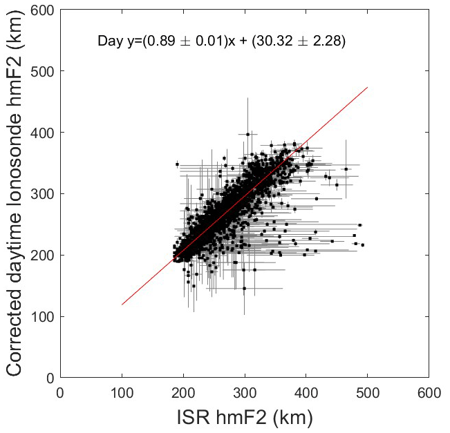
Figure 10 Hourly monthly median ionosonde-derived hmF2 values, corrected for the presence of foF1, plotted against monthly mean hmF2 values determined from the ISR; the correction results in a revised gradient of 0.89±0.01 with an offset of 30.32±2.28 km (given by the red line).

3.2 Long-term bias

The above analysis has established that there are biases in the empirical hmf2 formula for values of $fo\mathrm{F}\mathrm{2}/fo\mathrm{E}$ and $fo\mathrm{F}\mathrm{2}/fo\mathrm{F}\mathrm{1}$ below thresholds of 2.5 and 1.6, respectively. It has been shown that these introduce systematic errors on a seasonal and diurnal basis. It is therefore pertinent to the discussion of long-term change in the ionosphere to now consider how such biases may influence the long-term trends in hmF2 values derived via an empirical formula. Figure 9 presents the $fo\mathrm{F}\mathrm{2}/fo\mathrm{F}\mathrm{1}$ and $fo\mathrm{F}\mathrm{2}/fo\mathrm{E}$ ratios against the year for hourly monthly median values (top panels), the annual average (middle panels), and the percentage of observations (where a ratio can be calculated) for which the ratio is less than the threshold below which a bias is introduced into the empirical hmF2 equation (≤1.6 for $fo\mathrm{F}\mathrm{2}/fo\mathrm{F}\mathrm{1}$, as identified in Fig. 4, and ≤2.5 for $fo\mathrm{F}\mathrm{2}/fo\mathrm{E}$, as identified in Fig. 7). It can be seen that there is a strong solar-cycle dependence in both of these ratios, together with longer-term changes, particularly the apparent step change since the year 2000. The result of this is that some years will be far more susceptible to the systematic errors introduced into the empirical formula. The lower panels demonstrate that the percentage of data (for which ratios can be calculated) falling below these thresholds can vary from around 10 % to 100 %.

The relationship between the bias in hmF2 and the $fo\mathrm{F}\mathrm{2}/fo\mathrm{F}\mathrm{1}$ ratio established above was used to correct affected hmF2 values (where $fo\mathrm{F}\mathrm{2}/fo\mathrm{F}\mathrm{1}\le \mathrm{1.6}$) before averaging by year. When daytime values are plotted against the ISR hmF2 values (Fig. 10), the correction results in a revised gradient of 0.89±0.01, with an offset of 30.32±2.28 km.

Figure 11 The same as Fig. 10 but this time corrected for the bias introduced for values of the $fo\mathrm{F}\mathrm{2}/fo\mathrm{E}$ ratio below 2.5. The correction results in a revised gradient of 0.97±0.01, with an offset of 0.68±2.67 km (given by the red line).

Applying the $fo\mathrm{F}\mathrm{2}/fo\mathrm{E}$ correction to data results in an even closer fit between these data sets (Fig. 11). The gradient of the fit is 0.97±0.01, with an offset of 0.68±2.67. This improvement over the correction due to the presence of an F1 layer is likely due to the fact that $fo\mathrm{F}\mathrm{2}/fo\mathrm{E}$ values exist for a larger proportion of the daytime data points (∼64 %) than $fo\mathrm{F}\mathrm{2}/fo\mathrm{F}\mathrm{1}$ values (∼42 %).

While both these corrections have improved the relationship between the empirically derived and directly measured hmF2 values, the remaining gradient is not 1:1. This is unsurprising since there are other approximations that have been made when determining the coefficients within the empirical relation (which are likely to be specific to the dip angle of the local magnetic field) and in deriving M(3000)F2 values from the ionograms (which does not account for the presence of the magnetic field). In addition, we have not corrected for the small but systematic bias in hmF2 introduced by the signal delay in the ISR data.

It can be seen from Fig. 5 that the nighttime ionosonde-derived hmF2 values still show more scatter when compared with those measured by the ISR. As shown in Fig. 2, using a value of foE=0.4 MHz in the empirical formula tends to introduce more uncertainty into the hmF2 estimates, which results in an underestimate of the F2 layer height on average.

3.3 Influence of Earth's magnetic field on long-term hmF2 estimates

Standard calculations of M(3000)F2 do not take account of the influence of Earth's magnetic field on radio propagation, and it has long been known that this can introduce a bias into the estimation of this parameter from ionograms (Davies, 1959). More recently, Elias et al. (2017) modelled this bias and quantified the subsequent error introduced into estimates of hmf2. In order to estimate the influence of the magnetic field on hmF2 calculations for the location used in this study, the international geomagnetic reference field (IGRF, Thébault et al., 2015) was used to determine long-term magnetic-field variations at an altitude of 250 km above Kokubunji. Throughout the epoch of this study, the inclination has remained relatively stable, declining from 48.7 to 48.4° between 1957 and 1980 and subsequently rising to 49.6° by 2020. Using the figure presented in Elias et al. (2017), this would result in a systematic offset in hmF2 of ≤1 km, well within the uncertainties of the measurements. Further to this, modelling work by Cnossen and Richmond (2008) and Elias (2009) indicates that changes in Earth's magnetic field over Kokobunji would not be expected to affect the observed values of hmF2 through thermospheric dynamics for the epoch covered by this study. It is therefore assumed that there is no measurable bias caused by magnetic-field changes in the long-term variation in hmF2.

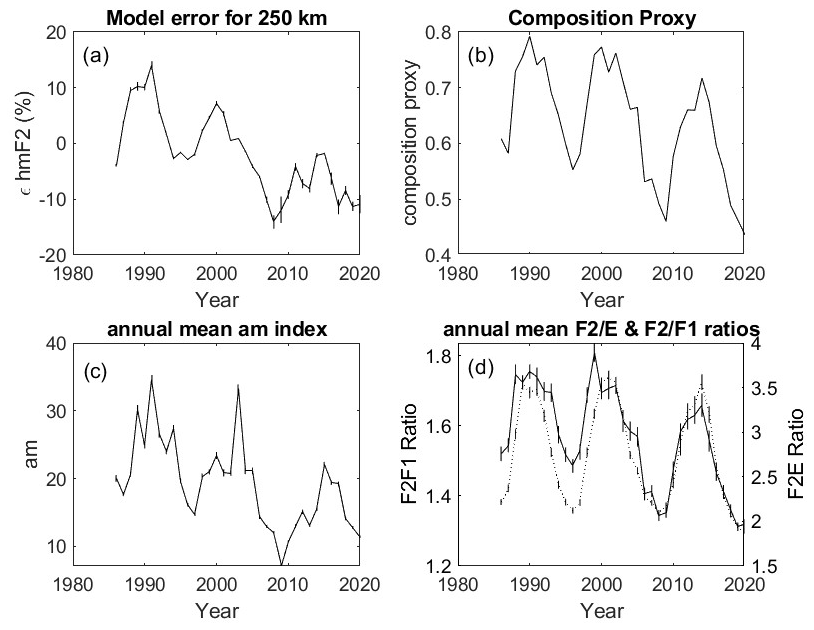
Figure 12 (a) Percentage error in the empirical hmF2 model, ϵhmF2, after calibration with ISR data for each year in the time range 1986–2020. (b) Qualitative composition proxy based on annual average noon foF2 value scaled by solar f10.7 cm flux. (c) Annual average values of the am index for the same epoch. (d) The annual average ratios in $fo\mathrm{F}\mathrm{2}/fo\mathrm{F}\mathrm{1}$ (solid line) and $fo\mathrm{F}\mathrm{2}/fo\mathrm{E}$ (dotted line) for the same epoch.

3.4 The impact of $fo\mathrm{F}\mathrm{2}/fo\mathrm{F}\mathrm{1}$ and $fo\mathrm{F}\mathrm{2}/fo\mathrm{E}$ biases on the long-term drift in estimates of hmF2

The suppression of foF2 values during the summer months and the seasonal variation in the presence of the F1 layer are both indications of a change in thermospheric composition. Having shown that these can lead to a systematic bias when using an empirical formula to estimate hmF2, this raises the question as to whether such a bias would be introduced into the study of long-term change in the height of the F2 layer.

In order to investigate this, the relationship between the ISR and ionosonde-derived hmF2 values was determined for each of the 35 years of common data. For each year, (uncorrected) monthly median ionosonde-derived hmF2 values were plotted against mean ISR measurements for all hours and months where there were data from both instruments. For each year, a linear fit was made between ionosonde-derived and ISR hmF2 values. The resulting gradient and offset of each fit were used to derive a modelled height for an arbitrary ISR height of 250 km. The differences between these two values were used to reconstruct the percentage error in hmF2. The results of this analysis are presented in Fig. 12a. It can be seen that there are solar-cycle variations in the model error, with an amplitude of ±10 % (±25 km at 250 km). This is of the order of decrease expected from climate change. Moreover, there is a long-term drift in this error which would undoubtedly introduce a bias into any estimates of long-term change in the height of the F2 layer. The question then arises as to what could be the cause of this long-term change in the formula error. Figure 12c presents the annual average of the geophysical am index (Lockwood et al., 2019). Here, we choose to use the am index rather than the Ap index used in previous studies. The response patterns of the individual magnetic observatories used to compile such indexes depend strongly on the level of geomagnetic activity. At low activity levels, the effect of solar zenith angle on ionospheric conductivity dominates over the effect of station proximity to the midnight sector auroral oval, whereas the converse applies at high activity levels. It has been shown (Lockwood et al., 2019) that these biases are far smaller for the am index than for Ap.

There is a strong and significant correlation (0.77, p≪0.0001) between the am index and the model error, suggesting that it is geomagnetic activity that is driving this variation in the accuracy of the empirical formula. If this long-term bias is consistent with the seasonal and diurnal bias of hmF2 estimates demonstrated in the earlier section of this paper, it would be reasonable to assume that the formula is being affected by changes to the underlying ionization profile, introduced by long-term changes in thermospheric composition arising, in turn, from long-term changes in geomagnetic activity. Figure 12b presents a qualitative proxy for the annual average thermospheric composition calculated from the square of monthly median noon foF2 values scaled by the solar f10.7 cm flux (Wright and Conkright, 2001). It can be seen that this proxy reveals very similar characteristics of a solar-cycle variation combined with a long-term decline (the correlation between these data and the model error is 0.835, p≪0.0001). More directly related to the earlier result that a bias is introduced into the empirical hmF2 formula by the presence of an F1 layer, Fig. 12d presents the annual average foF2 $/$ foE and foF2 $/$ foF1 ratios. These too demonstrate similar solar-cycle variations combined with, for foF2 $/$ foF1 in particular, a long-term decrease (foF2 $/$ foF1 correlation with model error is 0.86p≪0.0001; foF2 $/$ foE correlation with model error is 0.70p≪0.0001).

The sensitivity of thermospheric-composition changes to geomagnetic activity varies with geomagnetic latitude (e.g. Zuzic et al., 1997), with a station at low geomagnetic latitude being less prone to changes in molecular species at F region altitudes than a station at a high geomagnetic latitude.

For example, Slough–Chilton is a mid-latitude station in a geographic longitude sector near to the geomagnetic pole (at a geomagnetic latitude during this epoch of ∼48–50° N). Here, there is an annual variation in ionization, with ionospheric densities being greatest in the winter. In the summer, the greater concentration of molecular species in the thermosphere increases the ionospheric loss rate, resulting in lower F region ionospheric densities in the summer months, where the proportion of molecular species is relatively high. In the winter months, downwelling of the meridional thermospheric circulation results in a thermospheric composition dominated by atomic species which have a lower loss rate. This seasonal change in composition exceeds the variation in ion production due to the seasonal change in solar zenith angle over the same period.

In contrast, Stanley in the Falkland Islands (at a geomagnetic latitude of ∼35–39° S during this epoch) is a station that is far enough from the magnetic pole that compositional changes between the equinox and winter months are relatively small compared with the associated change in solar zenith angle, resulting in a semi-annual variation in foF2 (Millward et al., 1996). The relative magnitudes of the annual and semi-annual variations at a given station vary depending on geomagnetic activity, resulting in the long-term trends identified by Scott et al. (2014).

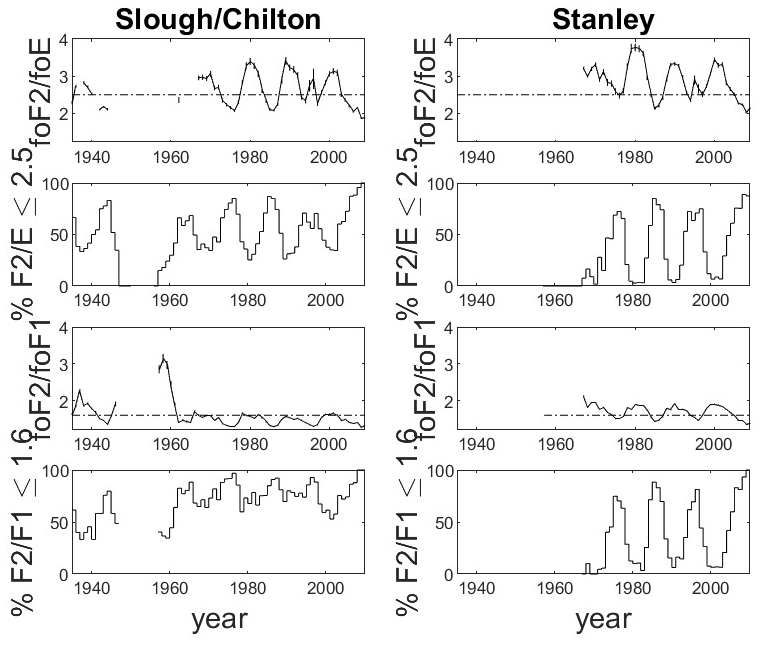
Figure 13 Annual mean foF2 $/$ foE (top row) and foF2 $/$ foF1 (third row) ratios calculated from monthly hourly median data for two stations: Slough–Chilton in the UK (left-hand column) and Stanley in the Falkland Islands (right-hand column). Ratios of less than 2.5 (for foF2 $/$ foE) and 1.6 (for foF2 $/$ foF1) have been shown to introduce bias into the empirical formula used to calculate hmF2 from ionosonde data. There are marked differences in the sensitivity to these biases between the two stations. The foF2 $/$ foE and foF2 $/$ foF1 ratios remain below the respective thresholds for more of the data in the Slough sequence, making it far more sensitive to bias in hmF2 calculations than Stanley, where the ratio is above the thresholds for a far greater proportion of the data. The fraction of the data (for which each ratio can be calculated) also varies with time (second and fourth rows), which will lead to a bias in any long-term trend in hmF2 calculated using the empirical formula. The sensitivity to this long-term bias will also differ between stations.

In contrast, the influence of compositional change on the peak concentrations of the E and F1 layers is much smaller since molecular ions exist in much greater proportions at these altitudes and because loss rates are higher due to the comparatively high thermospheric densities.

Such differences are also likely to influence the relative values of the foF2 $/$ foE and foF2 $/$ foF1 ratios at these stations. For example, the ratios at Slough–Chilton will be lower during the summer when compositional change suppresses foF2 while foE and foF1 are at their peak. Figure 13 presents the mean annual foF2 $/$ foE and foF2 $/$ foF1 ratios calculated for Slough–Chilton (left-hand column) and Stanley (right-hand panel). With 2.5 and 1.6 representing the critical values below which a bias is introduced into the empirical formula used to calculate hmF2 (via foF2 $/$ foE and foF2 $/$ foF1, respectively), it can be seen that Slough–Chilton will be far more susceptible to these biases than Stanley, where the mean foF2 $/$ foE and foF2 $/$ foF1 ratios are higher and where a greater proportion of the values lie above these thresholds (shown in the figure as dash-dotted lines in the first and third rows). In addition, both stations exhibit some long-term change in these ratios, which would introduce further bias into any estimates of long-term trends in hmF2. Such regional differences will need to be accounted for in any global analysis of hmF2 trends.

3.5 Accounting for signal delay in the estimate of hmF2 in the MU radar ISR data

As discussed previously, the above analysis has assumed that the propagation of the ISR radar pulses was not delayed by the presence of underlying ionization, which, for the frequency of the MU radar (46.5 MHz), is expected to introduce a small but systematic offset. Since it is the bias in the height of the F2 peak we are interested in, the signal delay needs to be integrated along the path of the radio wave between the ground and the F2 peak, accounting for the upward and downward path of the signal.

By modelling the delay introduced into the time of flight by the signal interacting with the underlying ionization and comparing this with the known (modelled) height of the layer, an estimate can be made of this bias over a range of diurnal, seasonal, and solar-cycle conditions. While this is not an absolute measure of the delay occurring in the real-world data, it is sufficient to estimate the relative change in bias across a representative range of conditions.

In order to estimate this offset, the simplified Appleton–Hartree equation was applied, where

$$\begin{array}{}\text{(13)}& {\mathit{\mu }}^{\mathrm{2}}=\mathrm{1}-{\displaystyle \frac{kN}{f^{\mathrm{2}}}},\end{array}$$

where k=80.5, N is the electron concentration (m⁻³), and f is the radar frequency (Hz). Applying the binomial expansion, this can be approximated to

$$\begin{array}{}\text{(14)}& \mathit{\mu }=\mathrm{1}-{\displaystyle \frac{\mathrm{40.3}N}{f^{\mathrm{2}}}}.\end{array}$$

Here, the second term on the right-hand side of the equation represents the range bias introduced as the radio wave passes through a plasma. In this way, one TEC unit (1e16 electrons per m²) delays the ISR signal by approximately $(\mathrm{1}e\mathrm{16}\times \mathrm{40.3})/(\mathrm{46.5}e\mathrm{6}{)}^{\mathrm{2}}=\mathrm{186}$ m.

In order to estimate the likely impact of such a bias in the data being considered, the 2016 International Reference Ionosphere (IRI2016) was used to generate electron concentration profiles at the location of the MU radar for dates between 1986 and 2020, corresponding to each month and hour considered in the study. Each ionospheric profile was then integrated from an altitude of 80 km up to the height of the maximum electron concentration in order to estimate the integrated range bias (doubled to account for the two-way travel of the radio pulse).

The resulting values vary between 0.6 and 11.5 km, with a median value of 1.47 km, varying as a function of peak electron concentration which, as expected, varies with the time of day, season, and solar cycle.

The matrix of height offsets was then subtracted from the hmF2 hourly monthly means derived from the ISR data, and the analysis was repeated. The results (see Appendix A) showed similar biases, with the coefficients of the linear fit exhibiting slight changes (gradient of 79.6 with an offset of −196.5 for the foF2 $/$ foE correction and a gradient of 46.6 with an offset of −74.1 for the foF|2 $/$ foF1 correction). While it is not appropriate to apply these corrections to the individual points in the 35-year time series (since these have not been range-corrected), as these are linear fits, the small changes to the coefficients will result in similarly small changes to the corrected values. The underlying conclusions concerning the impact of the foF2 $/$ foE and $fo\mathrm{F}\mathrm{2}/fo\mathrm{F}\mathrm{1}$ ratios on the empirical hmF2 formula are unaffected.

4 Conclusions

Empirical formulae used to estimate the height of the ionospheric F2 layer from standard parameters, scaled from ionograms, have necessarily had to make some assumptions about the underlying ionization profile. We have shown that, for at least one of the established empirical formulae, that diurnal, seasonal, and long-term biases are introduced into estimates of hmF2 that are of similar, if not greater, magnitude than those expected to be introduced by the long-term cooling resulting from increased levels of CO₂ and CH₄ in the lower atmosphere. While, in the case of the Kokubunji station, the long-term bias is well correlated with long-term changes in geomagnetic activity, the physical mechanism is via changes to the underlying ionization, driven by variation in thermospheric composition. This leads to diurnal, seasonal, and long-term variations in both the foF2 $/$ foE and $fo\mathrm{F}\mathrm{2}/fo\mathrm{F}\mathrm{1}$ ratios that are not accounted for in the empirical formula.

When conducting their analysis of the Kokubunji data, Xu et al. (2004) used the formula of Bilitza et al. (1979). While a direct comparison cannot be made with the current analysis, the variability in long-term trends observed by Xu et al. (2004) (difference between long-term trends in noon and midnight hmF2, with the seasonal variation at these two times being opposite to each other) is consistent with a maximum bias occurring around noon in the summer months. Xu et al. (2004) also conclude that geomagnetic activity was not significant in the regression model used to remove the effects of geomagnetic and solar variability. This could be attributed to their use of a different empirical model. Nevertheless, our analysis indicates that variations in the bias of hmF2 estimates is likely to be driven by geomagnetic activity.

As noted in the introduction, geomagnetic activity may also induce changes in global thermospheric circulation, with changes in the meridional wind modulating the height of F2 layer. Titheridge (1995) reviews the magnitude of these effects. A poleward wind would move ionization to lower altitudes, where the loss rate is higher. This would lead to a decrease in the peak F2 ionization. Under such circumstances, the foF2 $/$ foE ratio could potentially become sufficiently small such that, in addition to the genuine change in layer height, the empirical formula would start to underestimate hmF2. More work is needed to deconvolve the relative magnitude of these effects, but whether they are driven by changes in the wind field or local changes in composition, geomagnetic activity can lead to a long-term bias in estimates of hmF2 when using an empirical formula.

While the wider family of empirical formulae has not been tested in this work, there is evidence (McNamara, 2008) that at least some of these empirical formulae exhibit seasonal bias. Furthermore, there is evidence that, while being driven by geomagnetic activity, long-term change in ionospheric composition can be geographically localized, with individual stations exhibiting a wide range of responses to geomagnetic activity (Scott et al., 2014; Scott and Stamper, 2015). We conclude that the lack of consistency in global estimates of long-term changes in hmF2 results from the localized nature of the long-term changes in thermospheric composition not accounted for in the empirical formula used.

Jarvis et al. (1998) reported an altitude dependence in their estimates of long-term change in hmF2 and hypothesized about physical mechanisms that would explain this. Our results indicate that such mechanisms do not need to be invoked but rather that the bias introduced into the formula affects the percentage uncertainty in the estimate of hmF2, which would lead to a bias that would also be altitude-dependent.

It may be possible to use the relationship between the foF2 $/$ foE and/or foF2 $/$ foF1 ratios and the formula bias to correct for long-term changes in thermospheric composition for this station, and it is also likely that the equivalent ratios at other stations could be used to account for the global variations in this bias to produce a unified estimate of the rate of long-term change in hmF2. Caution should be used in such an exercise, however, since the bias in the formula varies with season and the time of day. In addition, the formula used was calibrated for a specific station, and the sensitivity to these biases may vary with location. Other variations in the formula should be tested in this way to determine their relative sensitivities to compositional effects. It would be interesting to see if the biases determined in the present study vary with location by conducting similar calibrations using other ISR stations.

With the potential for biases within these empirical hmF2 formulae, the ideal approach would be to determine such trends from alternative sources, such as directly from ISR measurements (which, as pointed out by Rishbeth, 1999, will require a few more decades of measurements before any trends can be considered significant) or through the labour-intensive process of inverting ionogram profiles. While this latter suggestion is theoretically possible for stations such as Slough–Chilton for which the original ionograms still exist, such a task is currently beyond the scope of this analysis, requiring careful digitization, scaling, and verification across many generations of instruments and data formats. While this work has not addressed any potential bias introduced by long-term changes to the thermospheric circulation or geomagnetic field, it has nonetheless demonstrated a bias in the formula that, through long-term changes in thermospheric composition, can lead to localized biases in the estimates of hmF2 which, in turn, can explain the lack of global consensus regarding long-term changes in the height of the ionosphere. Importantly, the results from this paper show that diurnal, seasonal, and long-term biases are introduced into estimates of trends in ionospheric heights that are of similar, if not greater, magnitude than those expected to be introduced by the long-term thermospheric cooling. These analysis issues must be addressed before ionospheric observations can be correctly interpreted in relation to long-term climate models.

Appendix A: Additional figures

In this section, additional plots are presented regarding the average seasonal and diurnal variation in individual ionospheric parameters used to estimate hmF2 values via the empirical formula and how the estimated range correction for the ISR (as detailed in Sect. 3.5) affects the observed biases between ISR and ionosonde-derived estimates of hmF2. As with the analysis described in the main body of the paper, monthly median values were calculated for each hour of data, and these monthly medians were averaged over the 35 years of common ionosonde and ISR data.

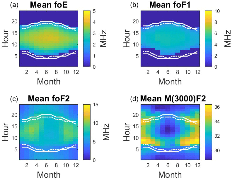
Figure A1 Hourly monthly median values of individual ionospheric parameters, averaged over the 35 years of common ionosonde and ISR data. The E layer peak frequency, foF2 (a, in MHz), peaks around noon in the summer months, corresponding to peak ion production (smallest zenith angle), and is absent at night. This same variation is seen for the F1 layer peak frequency, foF1 (b, in MHz), which is greatest around noon in the summer months. In contrast, the F2 layer peak frequency (c, in MHz) shows a minimum around noon in the summer months. The M(3000)F2 factor (d) is calculated from the ratio of the maximum usable frequency (MUF) and foF2. It, too, has a distinct minima around noon in the summer months.

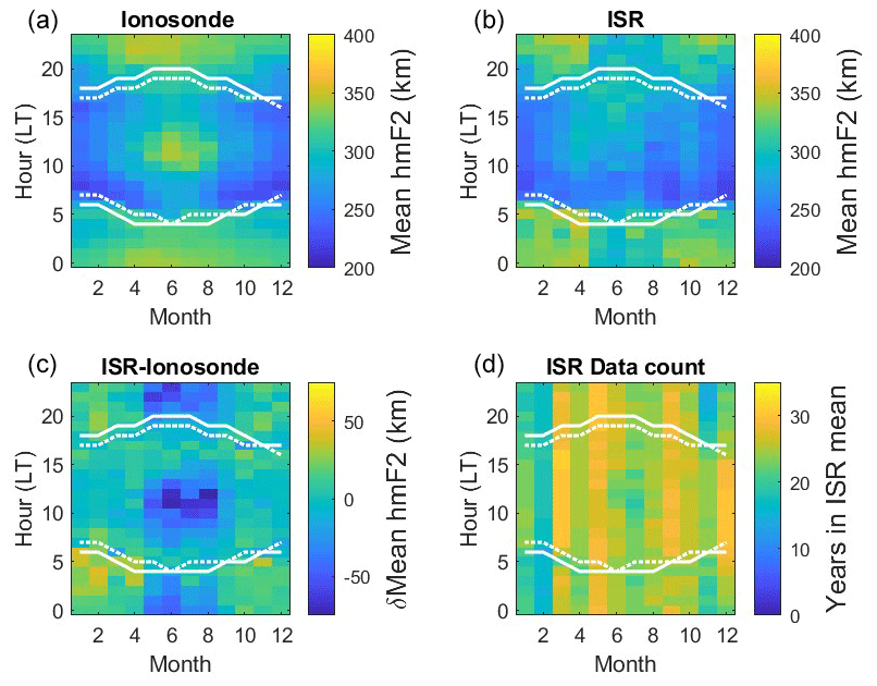
Figure A2 The same as for Fig. 3 but with the estimated ISR range corrections applied to each of the 12×24 bins in the seasonal and diurnal average data. Application of the estimated range correction has not significantly changed the observed seasonal and diurnal variations.

Figure A3 The same as for Fig. 4 but with the estimated ISR range corrections applied to each of the 12×24 bins in the seasonal and diurnal average ISR data. Application of the estimated range correction does not remove the observed bias below the threshold of foF2 $/$ foF1 =1.6, though the resulting fitted gradient changes to 46.6 with an offset of −74.1.

Figure A4 The same as for Fig. 5 but with the estimated ISR range corrections applied to each of the 12×24 bins in the seasonal and diurnal average ISR data. The corrected data are very similar in form, with the anomalous peak around noon in the summer months now being reduced, which better matches the ISR data.

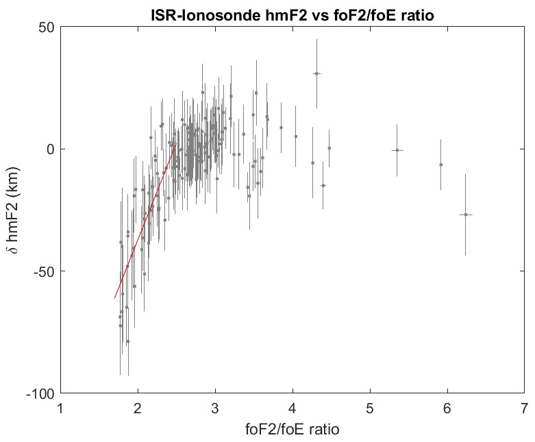
Figure A5 The same as for Fig. 7 but with the estimated ISR range corrections applied to each of the 12×24 bins in the seasonal and diurnal average ISR data. Application of the estimated range correction does not remove the observed bias below the threshold of foF2 $/$ foE =2.5, though the resulting fitted gradient changes to 79.6 with an offset of −196.5.

Figure A6 The same as for Fig. 8 but with the estimated ISR range corrections applied to each of the 12×24 bins in the seasonal and diurnal average ISR data. The corrected data are very similar in form, with the anomalous peak around noon in the summer months now being reduced, which better matches the ISR data.