the Creative Commons Attribution 4.0 License.
the Creative Commons Attribution 4.0 License.
 | 20 Feb 2024
Observations of polar mesospheric summer echoes resembling kilometer-scale varicose-mode flows
Jorge L. Chau
Ralph Latteck
Toralf Renkwitz
Marius Zecha
The mesosphere and lower thermosphere (MLT) region represents a captivating yet challenging field of research. Remote sensing techniques, such as radar, have proven invaluable for investigating this domain. The Middle Atmosphere Alomar Radar System (MAARSY), located in northern Norway (69∘ N, 16∘ E), uses polar mesospheric summer echoes (PMSEs) as tracers to study MLT dynamics across multiple scales. Chau et al. (2021) recently discovered a spatiotemporally highly localized event showing a varicose mode (simultaneous upward and downward movements), which is characterized by extreme vertical velocities () of up to 60 m s−1 in the vertical drafts. Motivated by this finding, our objective is to identify and quantify similar extreme events or comparable varicose structures, i.e., defined by quasi-simultaneous updrafts and downdrafts, that may have been previously overlooked or filtered out. To achieve this, we conducted a thorough manual search through a MAARSY dataset, considering the PMSE months (i.e., May, June, July, August) spanning from 2015 to 2021. This search has revealed that these structures do indeed occur relatively frequently with an occurrence rate of up to 2.5 % per month. Over the 7-year period, we observed and recorded more than 700 varicose-mode events with a total duration of about 265 h and documented their vertical extent, vertical velocity characteristics, duration, and their occurrence behavior. Remarkably, these events manifest throughout the entire PMSE season with pronounced occurrence rates in June and July, while the probability of their occurrence decreases towards the beginning and end of the PMSE seasons. Furthermore, their diurnal variability aligns with that of PMSEs. On average, the observed events persisted for 20 min, while the varicose mode caused an average expansion of the PMSE layer by a factor of 1.5, with a maximum vertical expansion averaging around 8 km. Notably, a careful examination of the vertical velocities associated with these events confirmed that approximately 17 % surpassed the 3σ threshold, highlighting their non-Gaussian velocity distribution and extreme nature.
- Article
(2934 KB) - Full-text XML
- BibTeX
- EndNote


As the boundary layer between the Earth's atmosphere and outer space, the MLT region is in many respects particularly interesting in terms of its dynamics and physical processes. On the one hand, the polar summer mesopause (78–88 km) is the coldest place in the Earth's system with temperatures as low as 130 K. These low temperatures are caused by dynamical processes such as the breaking of atmospheric gravity waves that bring the atmosphere out of thermodynamic equilibrium (Lübken et al., 1999). On the other hand, it is particularly difficult to continuously study this region of the atmosphere, as it is too low for satellites and too high for most in situ measurement methods such as balloons. The use of remote sensing techniques, particularly radar systems, has proven to be a notably advantageous and valuable approach in scientific MLT investigations. This is primarily due to their capability to effectively and continuously probe the altitudes of interest while being independent of weather conditions and the time of the day.
In the polar summer mesopause, cold temperatures create ideal conditions for the formation, growth, and sedimentation of ice crystals of different sizes. Ice particles larger than ≈ 20 nm can be observed with the naked eye as, e.g., noctilucent clouds (NLCs), at an altitude of about 82 km. These clouds are visible to the observer at high latitudes and midlatitudes as they are illuminated by the sun that has set during twilight and the night. Their occurrence and properties provide valuable insights into the composition and dynamics of the MLT region (Rapp and Lübken, 2004). Smaller ice particles are light enough to exist up to an altitude of around 90 km. They can be immersed in the D-region plasma, causing them to become charged. Additionally, in the altitude range of 80–90 km, gravity waves (GWs) are frequently observed propagating from lower atmospheric layers. These GWs become unstable and generate turbulence in the mesosphere. The turbulent velocity field transports charged ice particles, leading to small-scale structures in the spatial distribution of both the charged particles and the attached electron number density. This transport process leads to the occurrence of irregularities in the radio refractive index, which is effectively determined by the electron number density at these altitudes. These irregularities can cause radar echoes at a predominantly very high frequency (VHF) observed from the ground that are known as PMSEs. These are strongly influenced by the background conditions and thus by dynamical processes at different scales. Therefore, they are often used as tracers for dynamical processes within the MLT. A comprehensive overview of this phenomenon can be found in Rapp and Lübken (2004). However, it is important to emphasize that the occurrence of PMSEs is subject to daily and seasonal variations (Latteck and Bremer, 2017) and that they are most frequently observed within an altitude range of 80 to 90 km. The first echoes are typically seen around the middle of May, while the occurrence is maximal in June and July and fades in August (e.g., Latteck et al., 2021).
The observation of PMSEs by VHF radars serves as a unique tool for investigating horizontal and vertical wind velocities in the MLT, as the Doppler frequency shift of the radar echo is directly related to the radial (line-of-sight) velocity of the winds. This parameter can be determined using common methods of analyzing the magnitude spectrum of the received signal by, for example, determining its first moment or the phase slope of the autocorrelation function. When a radar beam is sufficiently narrow and pointed vertically, it can estimate the vertical wind speed component w. Additionally, the spectral width reflects the distribution of velocities, allowing for the evaluation of turbulence (Woodman and Guillen, 1974). The former in particular is not easy to obtain (e.g., Gudadze et al., 2019), although it has a significant influence on the energy budget and the deposition of momentum in the atmosphere (e.g., Garcia and Solomon, 1985; Chau et al., 2021). Numerous studies suggest that much lower velocities can be expected in vertical winds compared to horizontal winds. For example, mean meridional and zonal wind speeds are of the order of several tens of meters per second (e.g., Hoffmann et al., 2002; Jaen et al., 2022), whereas mean vertical wind speeds are typically below 5 m s−1 (e.g., Li et al., 2018; Chau et al., 2021). For this reason, most studies of mesospheric dynamics neglect vertical winds. Given this widespread assumption, the discovery of vertical wind velocities comparable to horizontal wind velocities was highly unexpected.
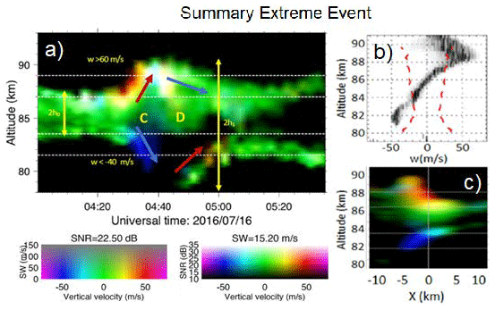
Figure 1Summary of an observed extreme vertical velocity event with MAARSY. (a) Time evolution of the vertical velocities between 75 and 95 km altitude over a time period of 1.5 h. Red and blue indicate the strong updrafts and downdrafts, respectively; green indicates vertical velocities around 0 m s−1, and the brightness of the colors represents the strength of the signal (SNR). (b) One example of the vertical velocity spectra during the event with 3σ presented as the dashed red lines. (c) A cut through the event showing the horizontal extent at one specific time (adapted from Chau et al., 2021).
In 2021, Chau et al. (2021) reported a single event observed by MAARSY in July 2016 over northern Norway. This event was characterized by uncommonly high vertical velocities, limited spatially and temporally between 80 and 90 km altitude as shown in a corresponding range–time–Doppler–intensity (RTDI) plot in Fig. 1. Vertical velocities moving away from the radar are shown in red, blue represents vertical velocities moving towards the radar, and green represents vertical velocities near 0 m s−1. The intensity of the colors corresponds to the signal strength (SNR). Figure 1c illustrates a two-dimensional plane from radar imaging, offering spatial information on the event. The updrafts and downdrafts exhibit clear localization both horizontally and vertically, measuring 3–4 km in width along the x axis and extending at least 8–12 km along the y axis.
The observed event, based on Doppler frequency measurements with MAARSY's vertical beam, shows simultaneous upward and downward movements, including vertical wind velocities reaching up to 60 m s−1 in the updraft (see Fig. 1). The extreme event visually resembles a mesospheric bore or soliton, with upper and lower surfaces oscillating out of phase by 180∘, as discussed by Dewan and Picard (1998), but with exceptional vertical velocities and extents. The fact that bores can form in the mesosphere was reported by, e.g., Taylor et al. (1995), Dewan and Picard (1998), and Fritts et al. (2020).
The discovery of the extreme event by Chau et al. (2021) provided motivation to explore older datasets from MAARSY to identify other extreme events. This motivation was further strengthened by the results presented in Feraco et al. (2018), where extreme vertical velocities under certain flow conditions and specific stratification values, particularly with a Froude number around 0.1 to 0.01, were predicted based on direct numerical simulations (DNSs). Emphasizing the limitations expressed by Chau et al. (2021), it is crucial to acknowledge the challenges associated with a direct comparison of our event with their study.
Additionally, Dong et al. (2021) simulated vertical velocities of around ±40 m s−1 using the Complex Geometry Compressible Atmosphere Model for Polar Mesospheric Clouds (CGCAM-PMC). These recent findings have brought attention to the possibility that such high vertical velocities may have been overlooked or misinterpreted in previous analyses. Traditionally, outliers or anomalies in a dataset have been identified as individual values exceeding 3 times the standard deviation (e.g., Lehmann, 2013).
Unpredictable short-term events with large impacts – in other words, extreme events – can occur in the upper atmosphere as well as in the lower atmosphere (e.g., tornadoes) and in the ocean (e.g., tsunamis). While research exists for the latter, in situ observation and studies of extreme events and small-scale dynamics in the polar MLT region are scarce.
Initially, the primary objective of this study was to investigate the frequency of events characterized by exceptionally high vertical velocities and small scales (referring to the spatial information taken from the radar imaging of the extreme event by Chau et al., 2021). It became apparent that such extreme events are not frequent. Instead, a recurring observation of events exhibiting a similar structure referred to as varicose (simultaneous upward and downward motion) emerged. The focus of this study is to provide a comprehensive report on these observations. As a new objective towards the ultimate goal, the aim is to gather as many characteristics as possible related to the occurrence of these events, particularly focusing on the associated vertical velocities, which originally motivated this work.
The dataset and methods used in this study are described in Sect. 2. The findings resulting from this analysis are presented in Sect. 3 and discussed in Sect. 4.
This study uses PMSE measurements obtained from MAARSY, a mesosphere–stratosphere–troposphere (MST) radar located on Andøya in northern Norway (69.30∘ N, 16.04∘ E). MAARSY is a monostatic, active phased array radar operating at a frequency of 53.5 MHz. Its design allows high flexibility in beam forming and beam steering as well as the use of modern interferometric applications for improved studies of the Arctic atmosphere with high spatiotemporal resolution (Latteck et al., 2012).
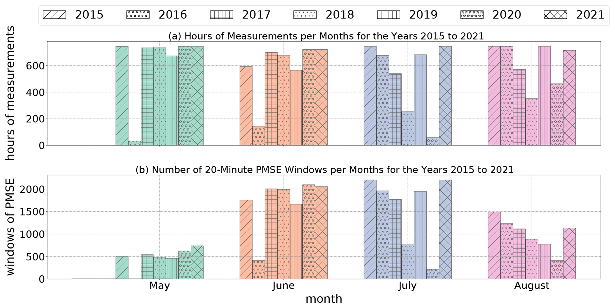
Figure 2(a) Number of hours during which the radar was operational and included in the data analysis and (b) number of 20 min windows in which PMSEs were detected and included in the data analysis, separately for each month of 2015 to 2021.
A collection of the main technical parameters of MAARSY and of the experimental configuration as used for the standard observation of PMSEs is given in Latteck and Bremer (2017).
The dataset used in this study consists of PMSE observations obtained during the summer seasons (i.e., May, June, July, and August) of 2015–2021 with 766 observation days. Notably, the number of observation hours during the mentioned period was not constant, as shown in Fig. 2a. Note that the measurement hours cover the radar's entire operational duration, including periods without PMSE detection (see Fig. 2b). The partly limited number of observation hours needs to be taken into consideration for the later interpretations of the results. In the years 2017, 2019, and 2021, nearly every day was included in the analysis. However, the first half of the PMSE season in 2016 and the second half of the seasons in 2018 and 2020 included only about one-third of the days. During these periods, special experiments were carried out with MAARSY characterized by a very low Nyquist frequency, which does not allow an analysis to be carried out with regard to extreme events.
The data used in this study are based on different radar experiments, all involving the vertical beam-pointing direction. A pulse repetition frequency (PRF) of 1 kHz and two coherent integrations (because of the use of complementary codes), resulting in a Nyquist frequency of fN=250 Hz, were predominantly used, enabling the determination of maximum vertical velocities of up to 700 m s−1. Exceptions to that are 3 months (June–August) in 2018, 1 month (July) in 2019, and 1 month (July) in 2020 when the PRF was adjusted to 828, 850, and 900 Hz, respectively, which modifies the temporal resolution and fN of the measurements.
In previous radar experiments, the raw data were additionally subjected to a high number of coherent integrations before undergoing further signal processing. This integration aimed to manage the amount of data effectively (Farley, 1985). However, this approach reduces fN and can lead to the filtering of unexpectedly high vertical velocities, as shown in Fig. 3. Since 2017, the standard MAARSY experiments for observing PMSEs have avoided additional coherent integrations, allowing for the reanalysis of a significant portion of the MAARSY dataset using the full Nyquist frequency fN=250 Hz, which corresponds to a maximum detectable radial velocity vrad=700 m s−1. However, the raw data from years prior to 2017 had a reduced fN, with values of 15.64 Hz (equivalent to vrad=43.8 m s−1) in 2015 and 62.5 Hz (equivalent to vrad=175 m s−1) in 2016, which allowed the discovery of the extreme event presented by Chau (2021). Data before 2015 were excluded from this study due to the substantial reduction in fN caused by a high number of coherent integrations. Within the observed period the altitude resolution is 300 m and the temporal resolution is on average ≈100 s mainly depending on the number of experiments and the duration they were running at a time.
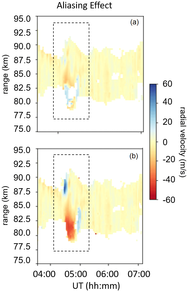
Figure 3The colored contours show the radial velocity observed on 16 July 2016 (a) after applying six additional coherent integrations (effective vrad≈30 m s−1) and (b) without applying additional coherent integrations (effective vrad=175 m s−1) over altitude. The velocities cannot be determined from the spectra due to filtering and are thus missing in (a).
For the determination of the Doppler velocity, we use the phase slope of the complex autocorrelation function. The search for additional extreme events has presented notable challenges, which arises from the stochastic nature of meteor occurrences, characterized by their unpredictable and sudden appearance with remarkably high radial velocities in the measurements. Occasionally, particularly strong echoes from off-vertical directions are received even through the well-attenuated radiation pattern side lobes. These echoes need to be flagged and removed from the further analysis. This introduces further complexity to the automation process, necessitating manual inspection for identifying notably high vertical wind velocities.
Following model expectations (e.g., Feraco et al., 2018; Dong et al., 2021), events similar to the extreme event reported in Chau et al. (2021) were found to be infrequent. Interestingly, lower-velocity events with the same varicose-mode structure, however, occurred more frequently. Varicose-mode events were considered to be phenomena that had simultaneous vertically ascending and descending winds, lasted only a few minutes, and were accompanied by a certain widening of the PMSE layer. To clarify the manual event selection process, Fig. 4 presents selected events and their simple schematics. The left column shows the example events in the form of aforementioned RTDI plots. The varicose structure is clearly evident in all three instances. Similar to the extreme event in Fig. 1, this type of structure causes the PMSE layer to expand during its presence and contract afterward. The outer boundaries of the PMSE layer are indicated by a black line, which is colored red and blue for updrafts and downdrafts, respectively, in the right column of Fig. 4. The vertical extent of the PMSE layer before and during the events is represented by 2h0 and 2h1, respectively. The start time of each event is marked as t0, and the duration of an event is denoted as d. With these denotations, we attempt to follow those in Fig. 1 (yellow vertical lines).
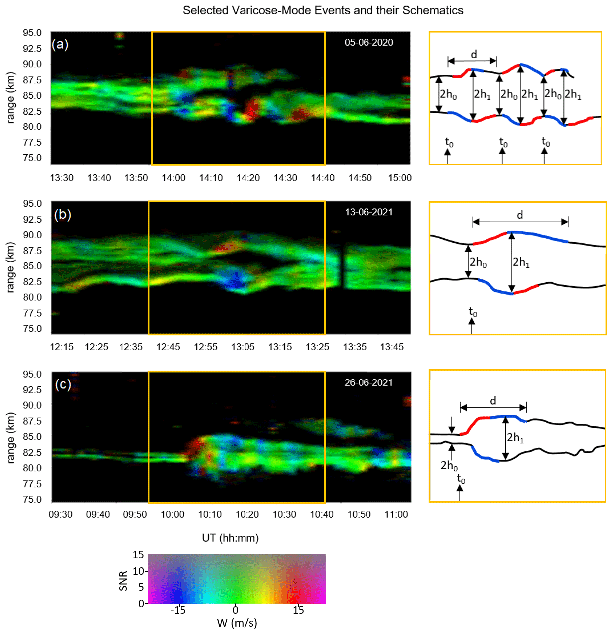
Figure 4Selected varicose-mode events: vertical velocity evolution (color-coded: red means upwards, blue means downwards, green means around 0 m s−1) between 75 and 95 km, exhibiting simultaneous upward and downward motions. Color brightness indicates signal strength. The observations were made on (a) 5 June 2020, (b) 13 June 2021, and (c) 26 June 2021. The right column shows event schematics with h0 and h1 representing undisturbed and disturbed PMSE layer thickness, respectively. t0 denotes event start time, and d represents duration. Red and blue indicate vertical wind direction, as in the left column.
The selection of varicose-mode events was a manual procedure mainly using the daily vertical velocity plots with a color bar chosen to range from −15 to 15 m s−1 to focus on events exceeding the 3σ threshold.
The data analysis involved an initial step of data masking, where only data points meeting specific criteria were retained for visualization. These criteria included a signal-to-noise ratio (SNR) not falling below −5 dB and vertical velocities not exceeding 100 m s−1. Consequently, data points falling outside of these established limits were excluded from the representation. This selective approach allowed for a clear depiction of PMSEs.
By zooming in on the figure, the temporal localization of events became more apparent, enabling the identification of event boundaries and the determination of the upper and lower extents of PMSEs before, during, and after each event. For instance, the PMSE layer's width immediately prior to an event's initiation (t0) was denoted as 2h0, while 2h1 represented the maximum width of the event, measured from the first pixels at the upper and lower edges. Typically, the widest point corresponds to the juncture of the initial updraft and downdraft phases within the event. In some instances, updrafts and downdrafts did not occur simultaneously but rather quasi-simultaneously, exhibiting a slight temporal offset relative to each other. In such cases, the midpoint of the event might not coincide with the point of maximum width.
Upon identifying and characterizing an event within its spatial and temporal dimensions, further steps were necessary to determine the maximum vertical velocities. As previously mentioned, employing an automated search method posed challenges due to the sporadic occurrence of meteors. These meteors have the potential to not only amplify the signal but also mimic exceptionally high vertical velocities. To ensure that these meteor events did not influence the study of varicose-mode events, the power-time plots forming the basis of the spectra used for velocity determination were meticulously examined for characteristics primarily associated with short-term, intense signals across multiple altitude channels. When a presumed velocity maximum coincided with such a signature in the power-time plot, it was disregarded, and the subsequent smaller value was considered.
To address challenges in varicose-mode event observations related to diurnal and annual PMSE variability, as well as fluctuating observation hours, the event numbers are normalized to the occurrence of PMSEs within a specific time period. A PMSE within the MAARSY dataset was classified as such if it met specific criteria. The normalization process involved dividing the resulting daily PMSE-defining matrices into 20 min windows, focusing on the altitude range of 82 to 88 km with high PMSE occurrences. These restricted windows were analyzed for PMSEs, considering a 50 % threshold of PMSE-labeled pixels across all altitudes to indicate PMSE presence.
The analysis of the MAARSY dataset (2015–2021) revealed frequent occurrences of varicose-mode events. Figure 4 illustrates three characteristic events to demonstrate the recurring properties of typical varicose structures and their duration. These events are not limited to a single occurrence within a short period of time (e.g., 1 h), as shown in Fig. 4a, where structures can occur successively with only a few minutes to a few tens of minutes in between. The plots also highlight that while the structures themselves appear similar, their vertical extent and the presence of substructures, such as additional layers, vary from case to case. Information regarding occurrence, duration, vertical extent of the PMSE layer, and prevailing vertical wind speeds was collected for the identified events.
3.1 Varicose-mode event occurrence
The analysis of the 766 observation days revealed that varicose structures occurred on 249 d, indicating that these events take place on roughly 33 out of 100 d. Within the seven PMSE seasons, 707 varicose-mode events were observed. A detailed overview of their occurrence during the observation period is given in Figs. 5a–b and 6a. Supplementary data summarizing the values can be found in Table 1.
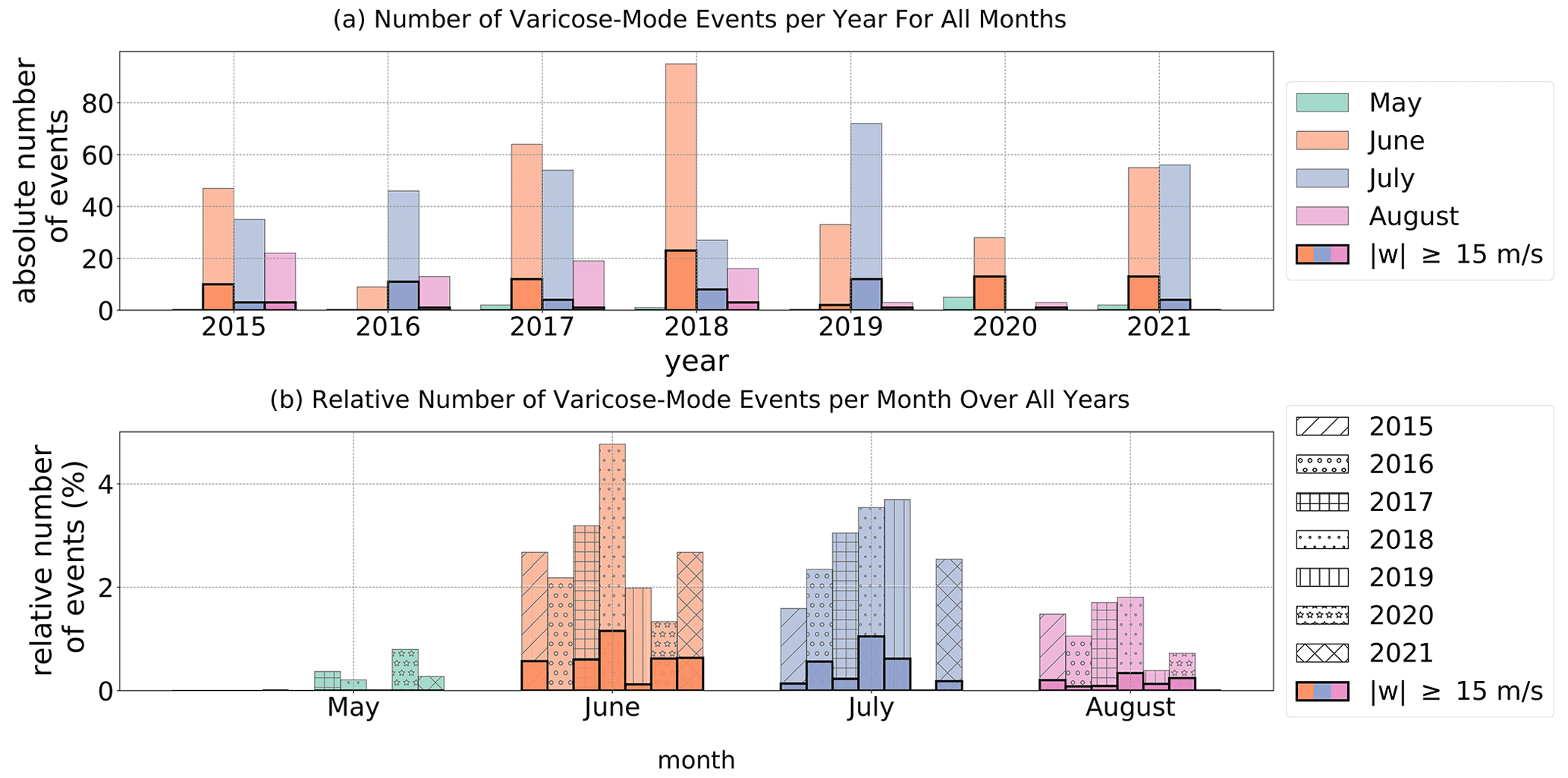
Figure 5Occurrence of varicose-mode events in the PMSE months (May, June, July, August) between 2015 and 2021. (a) The absolute number of events counted per year, broken down by individual months. (b) The number of events counted per month relative to the number of 20 min PMSE windows counted during the same period, broken down by individual years. The more heavily colored and contoured bars represent the absolute (relative) number of those events in the respective period with m s−1.
Figure 5a shows the absolute number of events per year, broken down by each month of the PMSE season. Events with vertical velocities m s−1 are visually highlighted by more intense colors and a thicker black frame. Please be aware that this principle will also be implemented in Figs. 6 through 9. The value of m s−1 has been selected as a conservative number that represents at least 3σ of standard values. It is noteworthy that events in varicose mode were observed in all years, with no discernible pattern. However, the total number of events per year showed variation, with a relatively high number of events observed in 2018 and only a few in 2020. In addition, the proportion of each PMSE month to the total number of events varied across the years.
Figure 5b shows the relative frequency of varicose-mode events versus the number of 20 min PMSE windows to provide a normalized perspective. Each month is shown with a unique color, while different patterns represent individual years. Most PMSEs occurred in June and July, with fewer events in August and the lowest frequency in May. On average, the probability of observing a varicose-mode event during the PMSE season was approximately 2.5 % in June and July, 0.3 % in May, and 1.0 % in August, given that PMSEs were detected.
Table 1Summary of the absolute numbers of varicose-mode events per month and year. In parentheses is the number of 20 min windows that contained PMSEs for the same time period (only the days included in this study). In the last column and row the total numbers are shown.
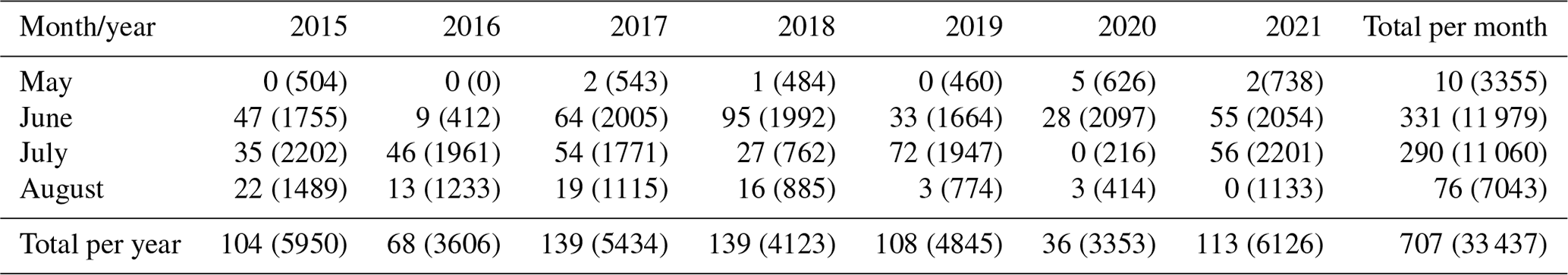
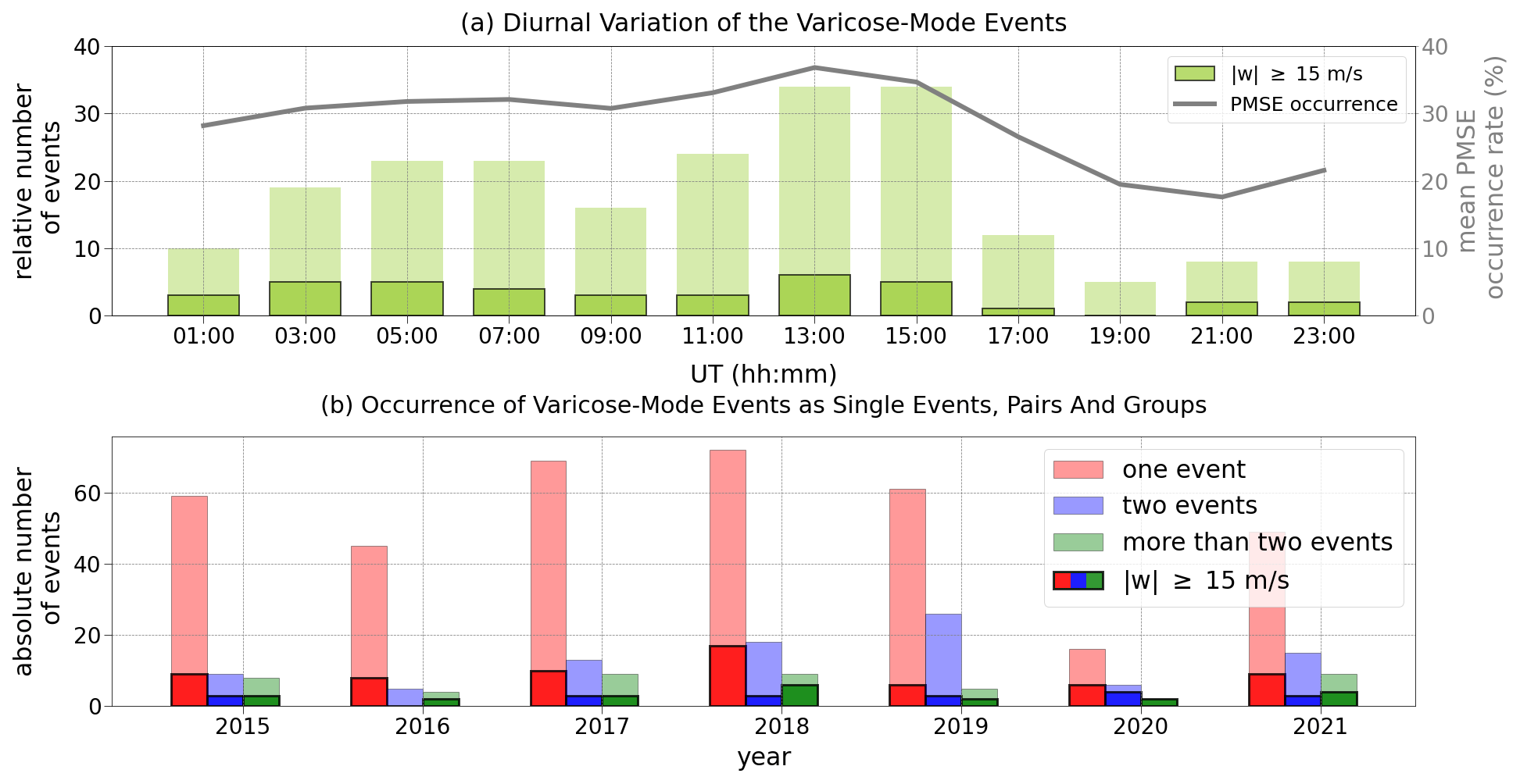
Figure 6(a) The distribution of the relative occurrence of events in varicose mode over the course of a day. The gray line illustrates the mean diurnal variation in the frequency of PMSEs by Latteck et al. (2021). (b) The absolute number of varicose-mode events occurring as single events, as pairs, or in groups for each individual year.
The diurnal variation of varicose-mode events is shown in Fig. 6a as relative numbers spread over a day throughout the 7-year period. The graph illustrates that these events can occur at any time of day. However, a clear peak is observed between 12:00 and 16:00 UT, while a minimum occurs between 18:00 and 20:00 UT. Varicose events can occur as single events, pairs (two events), or groups (more than two events), as shown in Fig. 4. The absolute numbers of these categories are shown in Fig. 6b for each year. In the case of Fig. 6b, the number of events with m s−1 is increased by one count if a single event within a pair or group has such high vertical velocities. In the varicose mode, single occurrences were observed predominantly (371 events, 52 % of the total), followed by event pairs (92 pairs, 26 % of the total). The least frequent are groups, with 46 counted instances (22 % of the total), which contain 3 to 8 events within a brief time frame.
3.2 Varicose-mode duration and vertical extent characteristics
Figure 7a shows the durations (see Fig. 4d) of the events found in this study. It was discovered that the events typically lasted an average of (20±9) min (see solid red line in Fig. 7a), ranging from a minimum of 4 min to a maximum exceeding 100 min.
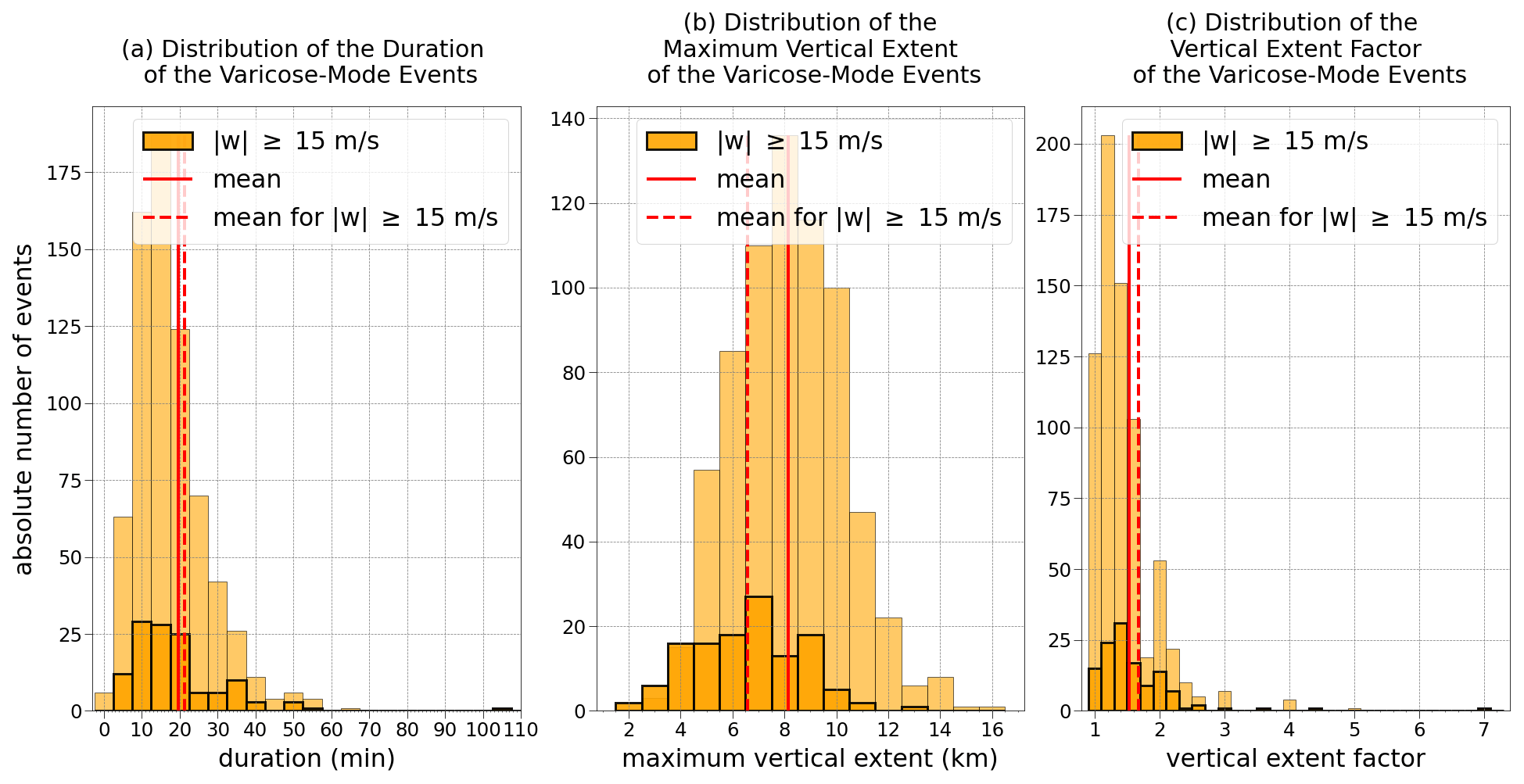
Figure 7Duration (a), maximum vertical extent (b), and (c) distribution of the varicose-mode events. The solid (dashed) red line represents the mean of all events ( m s−1 events).
The aforementioned PMSE layer characteristics during the events are summarized in Fig. 7b and c, showing the vertical expansion variations caused by the varicose structures. The solid red line in Fig. 7b represents the average maximum vertical PMSE layer thickness (see 2h1 in Fig. 4), which is approximately (8 ± 2) km, with values ranging from 3 to 15 km. The ratio between the initial vertical width of the PMSE layer (see 2h0 in Fig. 4) and its maximum width during an event (2h1) is depicted in Fig. 7c, indicating a mean vertical widening by a factor of about 1.5 ± 0.5, with a range spanning from a minimum of 1 to a maximum of 7. The respective mean values for events with m s−1 are represented by the dashed red lines in Fig. 7b and c.
3.3 Vertical velocities
The main focus of this study was to gain a comprehensive understanding of the variability of vertical wind velocities. In order to accurately interpret the velocities of individual events, it is important to first examine the overall distribution of velocities over the entire period and height range (82 to 88 km for seven PMSE seasons). This velocity distribution, shown in green in Fig. 8a, follows a normal distribution with the center at 0 m s−1 and a standard deviation of about 3 m s−1. However, closer inspection reveals that the distribution is not completely symmetric and that downward vertical velocities (negative values) are slightly more frequent.
Figure 8b shows the velocity distributions for the highest upward and downward velocities recorded during each varicose-mode event (two values per event), represented by red and blue bars, respectively. It is clear that most of the vertical velocities of the varicose-mode events fall within the range of about ±15 m s−1. The black line compares these values to a Gaussian reference, mirroring the distribution in Fig. 8a.
The vertical velocity distribution of varicose-mode events shows a wide range, with updrafts exhibiting a slightly broader distribution compared to downdrafts. In total, velocities of m s−1 were observed in 67 downdrafts and 90 updrafts. In 34 cases these velocities were observed simultaneously in the updraft and downdraft.
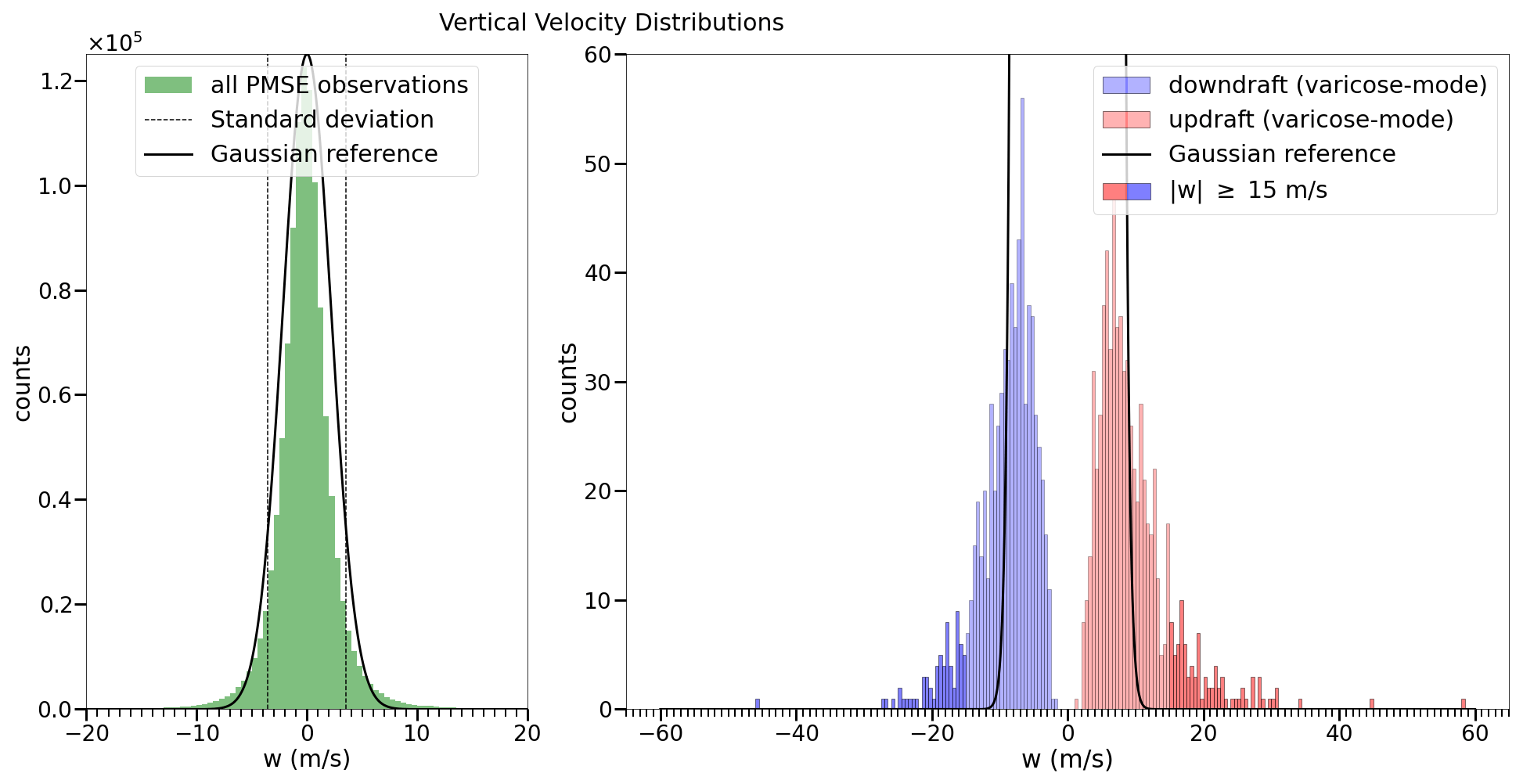
Figure 8Distribution (a) of vertical velocities across all altitudes and throughout the observation period and (b) of the maximum vertical velocities of varicose-mode events in blue (downdrafts) and red (updrafts). In both panels, the black curve represents a Gaussian reference.
3.4 High-velocity varicose-mode events
The distribution of vertical velocities in varicose-mode events is broad, with high-velocity events ( m s−1) accounting for about 17 % of the total varicose-mode event collection. Previous figures showing the distribution of all varicose-mode events over different timescales (year, month, or day), as well as providing information on their duration, vertical extent, and vertical extent change, also show events characterized by vertical velocities of m s−1. These are highlighted in the figures by more intense colors and thicker outlines of the bars.
It was found that high-velocity varicose-mode events occurred every year and can be observed in any month of a PMSE season except May (see Fig. 5a and b) and at any time of the day except for 18:00 UT (see Fig. 6a). Additionally, they can be found as single events, in pairs, or in event groups (see Fig. 6b). Specifically, 65 events were counted as single occurrences, constituting approximately 9 % of the total count of single events. For event pairs, the proportion is approximately 20 %, while group instances account for around 47 %. Transitioning from single events to event groups, there is a decrease in the absolute number of occurrences within each category, while the proportion of high-velocity events increases.
On average, these remarkable events last about (22 ± 13) min (see Fig. 7a), reach a maximum vertical extent of about (6.5 ± 2) km (see Fig. 7b), and experience a change in vertical extent by a factor of about (1.7 ± 0.7) (see Fig. 7c).
Figure 8b shows that updrafts have more absolute velocities above 15 m s−1 than downdrafts (42 vs. 39). While these numbers seem very similar, the distribution of events with m s−1 appears to be broader for upward winds because of a higher number of velocities above 20 m s−1. Specifically, there are 7 downwind and 17 upwind events in the latter category.
Motivated by the occurrence of an extreme event showing high vertical velocities in a varicose structure, this study has undertaken an extensive manual search for other events. It has become evident that the predictions made by DNS and models held true and that such events do not occur frequently. The study encompasses a dataset spanning the PMSE months between 2015 and 2021. However, the significance of this study lies in the observation of localized, temporally restricted structures characterized by a varicose mode.
4.1 Varicose-mode events and instabilities
In comparison to other studies, these structures bear the closest resemblance to mesospheric bores, a concept proposed by Dewan and Picard (1998). Their study introduced the term internal mesospheric undular bore to describe an event observed in airglow measurements, characterized by a sharp wave crest followed by smaller trailing waves. This event had contrasting effects on different layers of the atmosphere. It increased the brightness of the OH layer at 85 km and the Na layer at 90 km but had the opposite effect on the O and OI layers at 94 and 96 km, as reported by Taylor et al. (1995). Dewan and Picard (1998) drew parallels between these airglow observations and phenomena observed in the troposphere and water, such as undular tidal bores in riverbeds and “morning-glory” clouds. They suggested that these mesospheric bores require a channel-like structure, potentially provided by a thermal or Doppler duct, caused by a temperature inversion layer (also known as a mesospheric inversion layer, MIL) or wind shear. The theory of a duct for a guiding structure was initially confirmed by She et al. (2004) through the observation of temperature inversion layers coinciding with the occurrence of two mesospheric undular bore events over Fort Collins, Colorado, in 2002. This finding is further supported by Hozumi et al. (2019), who studied spaceborne airglow observations and found that most mesospheric bores observed between 55∘ N and 55∘ S occurred within such inversion layers. In contrast to the observations made by Dewan and Picard (1998), the trailing waves, as the bore-defining feature, are not evident in all of the observations in this study. Instead, they mostly appear as unattached wave crests, characteristic of solitary waves that occasionally result from bores (Koch et al., 2008).
In this study, the observed events can be described as solitary waves in a varicose mode, meaning quasi-simultaneous upward and downward movements (Lighthill, 1979). To investigate potential ducting mechanisms during the observed events, temperature measurements within a small radius around the MAARSY site and close-range measurements of the horizontal wind components are essential. Fortunately, data from the Spread-Spectrum Interferometric Multistatic Meteor radar Observing Network (SIMONe), operated by the Leibniz Institute of Atmospheric Physics (IAP) in close proximity to MAARSY, can be utilized for this purpose. Additionally, data from an iron lidar operated by IAP, located near MAARSY, could be examined to identify mesospheric temperature inversion layers in the future.
A further step towards understanding the underlying physics of these varicose (including extreme) events is to use the collected background conditions to attempt a replication of the varicose-mode structures and the exceptionally high vertical velocities through DNS. Initial attempts have been recently performed by Ramachandran et al. (2023). Using a two-dimensional DNS of the Navier–Stokes equation with the Boussinesq approximation, they successfully replicated key characteristics of a mesospheric bore event observed in OH airglow over Kühlungsborn, Germany, in March 2021. Their findings highlight the influential role of the temperature duct width and the amplitude of the initial perturbation in shaping the evolution and morphology of the bore.
4.2 Occurrence statistics
The analysis of more than 700 varicose structures in the MLT region revealed an overall occurrence rate of approximately 33 in 100. Although there is no discernible pattern in events across years, fluctuations in the total number of events per year were observed. The higher occurrence of events in 2018 and the relatively few events in 2020 demonstrate this variability. These lower event counts in 2020 (see Fig. 5a) may be attributed to the reduced dataset included in this study (see Fig. 2a). This explanation is challenged by the maximum number of events observed in 2018, despite a comparatively low number of observation hours included in this study. The implications of this discrepancy require further investigation. Individual months also contributed differently to the total occurrence, highlighting the influence of temporal factors on the occurrence of varicose events.
The concentration of events in the middle of the PMSE season, particularly in June and July, is consistent with previous studies that have identified these months as peak periods for PMSE activity. It is important to note that varicose-mode event occurrence was analyzed in relation to the number of 20 min PMSE windows, and a normalization factor was applied to account for diurnal and seasonal variations in PMSE occurrence. This normalization ensures the validity and comparability of event counts per PMSE season or month. The methodology included validation of PMSE occurrence within specific time periods using a threshold-based approach (see Sect. 2). The density of events is thus higher in the second half of the PMSE season than in the first half. When considering events as individual occurrences, pairs, or groups, the relative numbers of high-velocity events increase, although their absolute numbers are lower.
The observed diurnal pattern, with a maximum occurrence between midday and 16:00 UT and a local minimum between 18:00 and 20:00 UT, aligns with the known diurnal variability of PMSEs over Andøya indicated by the gray line in Fig. 6 (e.g., Hoffmann et al., 1999; Latteck et al., 2021). The significant variability in event counts relative to the average rate of PMSE occurrence strongly suggests a compelling link between varicose-mode events and the factors influencing PMSE patterns. This implies that both phenomena likely share common underlying mechanisms, indicating a potential interdependence between them. However, the limited dataset and reliance on PMSEs as a tracer prevent conclusive statements about annual, interannual, or diurnal periodicity.
If assuming these events are mesospheric bores, comparisons can be drawn regarding occurrence rates to a recently published study by Hozumi et al. (2019), who examined the occurrence probabilities of mesospheric bores observed using airglow imagers on the International Space Station. Note that the absence of evidence confirming the varicose structures as bores and the limited satellite observations (55∘ S to 55∘ N) outside MAARSY's range should be considered. Nevertheless, this suggests that if the structures found in this study are bores, they may also occur frequently in midlatitudes and equatorial regions, with a preference for middle and equatorial latitudes during equinox seasons. Regarding diurnal variations, Hozumi et al. (2019) found a stronger dependence on daytime at midlatitudes compared to near the Equator.
The study, initially motivated by a singular extraordinary event, unexpectedly discovered occurrences of events in pairs or groups. The close time intervals between individual events within a pair or group suggest conditioning and influence from one event to the next. The possibility of memory involvement and differences in the origin of isolated events versus events in pairs or groups are intriguing. Group events exhibit a distinct pattern with a leading wave crest and trailing waves, resembling bores. However, the amplitudes of the supposed trailing waves are nearly equivalent to the leading wave (see Fig. 4a), contrary to previous reports (e.g., Taylor et al., 1995; Dewan and Picard, 1998). The significance of these statistics is yet to be determined.
The occurrence patterns of high-velocity events ( m s−1) and varicose-mode events in general align, but there is no direct correlation with the absolute (Fig. 5a) or relative (Fig. 5b) number of the latter. In other words, a higher number of varicose-mode events does not necessarily correspond to a higher number of high-velocity events. An example can be seen in Fig. 5a for 2021, where the absolute number is higher in July compared to June, but this behavior is not mirrored by the events with absolute vertical velocities exceeding 15 m s−1 – there are significantly more of those in June than in July. Similarly, in the year 2020, no high-velocity events were observed in May, despite a larger absolute number of events compared to August. This lack of correlation is further highlighted in Fig. 5b, where it becomes apparent that years with a higher number of varicose-mode events per number of PMSE windows, such as in July, do not necessarily exhibit a higher occurrence of events with higher vertical velocities. The diurnal variation of high-velocity events is less pronounced compared to general varicose events, with a notable absence of them between 18:00 and 20:00 UT (see Fig. 6a).
Duration
The duration of varicose-mode events, averaging 20 min, demonstrates their relatively short-lived nature. This finding justifies the selection of a 20 min window size for counting PMSE occurrences, as it captures the majority of these events. Compared to the event described by Chau et al. (2021), which lasted approximately 25–30 min, this average duration is a bit smaller.
It is important to note that the radar illumination area in the mesosphere is relatively narrow (5.4 km diameter at 85 km altitude), and dynamical structures only pass through it, making them visible for a duration that depends on their speed through the field of view. The observed durations and vertical expansion variations in varicose-mode events provide valuable insights into their characteristics and potential underlying mechanisms. Mesospheric bores, for instance, can persist for several hours (e.g., simultaneous airglow and lidar observations by Smith et al., 2017; Fritts et al., 2020). The small observation volume in the mesosphere makes it challenging to determine exact lifetimes and to draw conclusions about the production and dissipation of the varicose-mode events.
In terms of duration, high-velocity events exhibit a similar average duration of around (22 ± 13) min compared to general varicose events but with a larger standard deviation. This prompts further investigation into the potential correlation between maximum vertical velocity and event duration.
4.3 Vertical and velocity characteristics
4.3.1 Vertical extent and extent change
The maximum vertical extent of the PMSE layer in varicose-mode events of (8 ± 2) km is smaller compared to the 12 km extreme event reported by Chau et al. (2021). Similarly, the expansion factor of the PMSE layer due to the varicose structure is, with a mean value of 1.5, significantly smaller than the factor of 3 observed in the extreme event. Notably, there is also a difference observed in the expansion factor between high velocity-events and general varicose-mode events. The former is slightly smaller (1.7 ± 0.7) than the latter. The contrary effect was found for the maximum vertical extent of the PMSE layer. The value for events with m s−1 lies at approximately (6.5 ± 2) km, which is about 20 % less than the value for all events.
The mechanisms influencing the expansion factor in varicose-mode events are not fully understood. It is believed that vertical velocities, horizontal wind properties, and temperature profiles play a role in determining the propagation duct in which these events are most likely to travel (e.g., Ramachandran et al., 2023).
The majority of bore observations are conducted using airglow, lidar, or satellites, providing a two-dimensional view in space. In such cases, only the initial height h0 is known by using, for example, half of the width of a temperature inversion layer (e.g., She et al., 2004), while the disturbed height h1 (for h0 and h1 see Fig. 4) remains unknown. To calculate the amplitude of a bore crest, a normalized bore amplitude (also referred to as bore strength) β of 0.3 is normally assumed based on models. This value serves as a measure to differentiate between turbulent and undular bores and is determined by using (e.g., Lighthill, 1979; Dewan and Picard, 1998). Radar-based bore observations allow for the direct determination of 2h1, avoiding assumptions in our observations. An average β of 0.53 for all observed varicose-mode events can be seen in Fig. 9 (see the solid red line). Significantly, events with m s−1 show a slightly higher average β of 0.68. This implies that if these structures are indeed bores, they exhibit a turbulent nature and the potential for wave breaking. However, an alternative theory proposed by She et al. (2004) suggests that for internal bores, β>0.3 can still sustain an undular bore configuration, as energy may leak out of the duct region.
Radar observations are limited to the radar field of view, making it uncertain whether these observed structures dissipate outside the observed area. A comparison to findings by Fritts et al. (2020) shows a similar β (0.7) in their study of bore observations done simultaneously by an all-sky imager and lidar. Although such a value suggests a turbulent solitary wave, the observation revealed undular bores, possibly due to the absence of a thermal duct, supporting a soliton development. This highlights the importance of investigating ducting conditions in case studies of the events analyzed in this study.
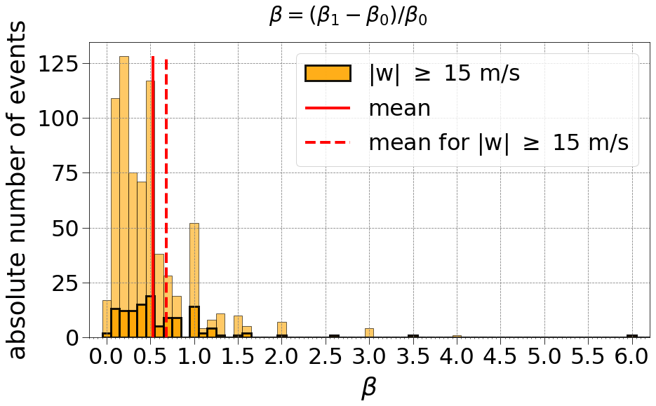
Figure 9Normalized bore amplitudes of the varicose-mode events in general. The solid (dashed) red line represents the mean of all events (events with m s−1).
4.3.2 Vertical velocities
Improving the accuracy of vertical velocity measurements using radar can be challenging due to several factors that contribute to uncertainty. The radar system itself contributes to some degree due to systematic errors, such as the variation of beam width and inaccuracies of beam orientation. To minimize this effect, MAARSY has been calibrated for transmission and reception. The pointing accuracy and nominal beam width have been verified by various experiments according to Renkwitz et al. (2017). While it is possible to determine vertical velocities by analyzing the Doppler shift of the received signal when the scatterer is directly over the vertically aligned radar beam, it is important to consider the limitations. Generally, the scatterers in the atmosphere are randomly distributed. Hence even with MAARSY's relatively narrow beam width, which is about 3.6∘, there is a possibility that scatterers will be detected that are not perfectly over the center of the radar location. Therefore, the measured radial wind will also contain a horizontal wind component, which depends on the mean angle of arrival as well as the magnitude and direction of the horizontal wind. Assuming the majority of scatterers are captured within the main beam and zenith angles of arrival predominantly fall below the radar beam's width, coupled with typical horizontal wind speeds below 100 m s−1, we can anticipate a maximum potential difference of approximately ±5 m s−1 between radial and vertical velocities. Consequently, it is reasonable to infer that the velocities under investigation in this study are primarily representative of the vertical component of the radial velocity, especially for velocities exceeding a few meters per second. Additionally, the identification of events in this study relied on visual assessment, which has inherent limitations. The choice of the color bar used in the visualization determined the detectability of varicose-mode events. A color bar ranging from −15 to 15 m s−1 was selected to focus on events exceeding the 3σ threshold, but it may have constrained the identification of events with lower velocities, which was deemed unnecessary given the study's objectives.
The observed mean vertical velocity of the varicose-mode events of 10 m s−1 is already twice as high as the expected maximum vertical velocity in the MLT, which was anticipated to lie within m s−1. In light of the extreme event reported by Chau et al. (2021) and the model predictions mentioned earlier, it is not surprising to observe instances with m s−1.
These magnitudes are notably high, surpassing more than 6 times the standard deviation of ≈ 2.5 m s−1 (see dashed black lines in Fig. 8). It is important to note that in the study conducted by Chau et al. (2021), vertical velocities were classified as “extreme” when exceeding 5 times the standard deviation. One could thus refer to the high-velocity events of this study as extreme as well.
Furthermore, it is observed that the occurrence of winds surpassing a threshold of ±15 m s−1 is comparable between updrafts and downdrafts. Nevertheless, downdrafts exhibit a narrower range of velocities compared to updrafts, primarily due to a larger quantity of updrafts with velocities exceeding 20 m s−1.
The general asymmetry of vertical velocities observed in this study (more downward- than upward-directed velocities in Fig. 8a) is consistent with previous findings. Gravitational sedimentation of ice particles forming PMSEs, as described by Gudadze et al. (2019), contributes to this asymmetry. The use of PMSEs as tracers in the vertical radar beam can introduce a bias towards downward-directed vertical velocities, as discussed by Hoppe and Fritts (1995), who used the EISCAT VHF radar. The authors suggest that gravity waves can cause a tendency to underestimate the upward motion when using VHF radars. This is because there is a negative relationship between the vertical motion caused by gravity waves and the radar's ability to detect them. They found that there is a correlation between certain types of vertical motions and radar measurements at different frequencies. For example, turbulence generated by upward-moving gravity waves can disrupt the radar's ability to measure them accurately. Additionally, it is plausible that in the case of downdrafts, regions with higher temperatures are quickly reached, leading to the melting of ice particles and subsequent dissolution of PMSEs. As a result, the tracer necessary to determine vertical velocities is again absent in such cases. Therefore, it is possible that the observed asymmetries may not be a true representation but rather a consequence of these influencing factors (e.g., Hoppe and Fritts, 1995; Gudadze et al., 2019).
To enhance the understanding of varicose-mode occurrence statistics, further analysis of additional MAARSY data, including previously excluded data, and data from preceding radar systems such as the ALomar WINd radar (ALWIN) is necessary. Expanding the research scope to incorporate other high-latitude MST radar data sources would also provide valuable insights. Considering the events' small-scale structure, radar imaging offers detailed insights into their morphology and spatial parameters in the horizontal plane, along with their motion direction within the radar beam. This imaging technique enables the resolution of smaller structures within a larger observation volume (e.g., Sommer and Chau, 2016). By using imaging combined with coherent MIMO (multiple input, multiple output) the angular resolution can be enhanced even further to around 1 km (Urco et al., 2019). Chau et al. (2018) presented another way of enhancing the quality of PMSE observations by combining MAARSY and the Kilpisjärvi Atmospheric Imaging Receiver Array (KAIRA) in a multistatic approach. This observation type would also enable the determination of a highly spatiotemporally resolved wind field of the polar MLT.
The main conclusion from this study emphasizes that the extreme event reported by Chau et al. (2021) is certainly not unique. After analyzing a radar dataset obtained from MAARSY during the PMSE seasons between 2015 and 2021, this study successfully confirms the occurrence of additional high-vertical-velocity events. Over the course of 7 years, spanning 4 months each, more than 700 incidents were identified that exhibited quasi-simultaneous upward and downward movements. Notably, a significant fraction of these events displayed absolute vertical velocities surpassing a threshold of 15 m s−1 (3σ), qualifying them as extreme.
Although the majority of the recorded cases featured velocities below the aforementioned threshold, detailed statistical analyses were performed separately for varicose-mode cases in general and those with large vertical velocities. Our analyses examined the occurrence statistics and vertical extent and vertical velocity characteristics of these events as well as their duration. It can be summarized that varicose-mode events occurred in every year covered by the study, regardless of the PMSE month or time of day, with some variability in both aspects. The occurrence of varicose-mode events seems to align with the occurrence of PMSEs, which in general held true for high-velocity events as well.
Further investigation into the duration, maximum vertical extent, and changes in vertical extent caused by the varicose structure () revealed an average duration of approximately 20 min (22 min for events with velocities exceeding 15 m s−1), an extent of around 8 km (6.5 km for events with velocities exceeding 15 m s−1), and a change in the maximum vertical extent of 50 % (70 % for events with velocities exceeding 15 m s−1).
With 2.5 %, the months June and July exhibit the highest likelihood of encountering extreme events also given the highest occurrence of PMSEs in general, thereby offering a favorable opportunity to conduct in-depth investigations and gather valuable data related to such phenomena. In order to comprehensively capture and examine extreme events through a well-coordinated campaign incorporating a multi-instrumental approach, the study at hand suggests that the optimal time window would fall within the months of June and July.
The data are available under https://doi.org/10.22000/1688 (Hartisch et al., 2024). The data to reproduce Figs. 1 and 3 were taken from https://doi.org/10.22000/396 (Chau, 2021).
JH identified, characterized, and analyzed the varicose-mode events described in the paper and led the writing. JLC contributed the main idea for analyzing varicose-mode events and helped structure the paper's organization. RL conducted radar experiments with MAARSY and performed preliminary analyses. TR performed a comparative analysis of radar data, verified the incident angle of arrival of radar echoes of selected events including receiver phase calibration, and aided in interpreting the study's findings. MZ processed the raw data, analyzed the autocorrelation functions, and calculated the radial velocities and signal-to-noise ratios. All authors have contributed to the improvement of the paper in written form.
The authors declare that they have no conflict of interest.
Publisher's note: Copernicus Publications remains neutral with regard to jurisdictional claims made in the text, published maps, institutional affiliations, or any other geographical representation in this paper. While Copernicus Publications makes every effort to include appropriate place names, the final responsibility lies with the authors.
This article is part of the special issue “Special issue on the joint 20th International EISCAT Symposium and 15th International Workshop on Layered Phenomena in the Mesopause Region”. It is a result of the Joint 20th International EISCAT Symposium 2022 and 15th International Workshop on Layered Phenomena in the Mesopause Region, Eskilstuna, Sweden, 15–19 August 2022.
Jennifer Hartisch thanks Kesava Ramachandran, Fabio Feraco, and Miguel Urco for helpful discussions.
The publication of this article was funded by the Open Access Fund of the Leibniz Association.
This paper was edited by Andrew J. Kavanagh and reviewed by two anonymous referees.
Chau, J. L., McKay, D., Vierinen, J. P., La Hoz, C., Ulich, T., Lehtinen, M., and Latteck, R.: Multi-static spatial and angular studies of polar mesospheric summer echoes combining MAARSY and KAIRA, Atmos. Chem. Phys., 18, 9547–9560, https://doi.org/10.5194/acp-18-9547-2018, 2018. a
Chau, J. L.: ChauGRL2021, Leibniz Institute of Atmospheric Physics at the University of Rostock [data set], https://doi.org/10.22000/396, 2021. a
Chau, J. L., Marino, R., Feraco, F., Urco, J. M., Baumgarten, G., Lübken, F., Hocking, W. K., Schult, C., Renkwitz, T., and Latteck, R.: Radar Observation of Extreme Vertical Drafts in the Polar Summer Mesosphere, Geophys. Res. Lett., 48, e2021GL094918, https://doi.org/10.1029/2021GL094918, 2021. a, b, c, d, e, f, g, h, i, j, k, l, m
Dewan, E. M. and Picard, R. H.: Mesospheric bores, J. Geophys. Res.-Atmos., 103, 6295–6305, https://doi.org/10.1029/97JD02498, 1998. a, b, c, d, e, f, g
Dong, W., Fritts, D. C., Thomas, G. E., and Lund, T. S.: Modeling Responses of Polar Mesospheric Clouds to Gravity Wave and Instability Dynamics and Induced Large-Scale Motions, J. Geophys. Res.-Atmos., 126, e2021JD034643, https://doi.org/10.1029/2021JD034643, 2021. a, b
Farley, D. T.: On-line data processing techniques for MST radars, Radio Sci., 20, 1177–1184, https://doi.org/10.1029/RS020i006p01177, 1985. a
Feraco, F., Marino, R., Pumir, A., Primavera, L., Mininni, P. D., Pouquet, A., and Rosenberg, D.: Vertical drafts and mixing in stratified turbulence: Sharp transition with Froude number, Europhys. Lett., 123, 44002, https://doi.org/10.1209/0295-5075/123/44002, 2018. a, b
Fritts, D. C., Kaifler, N., Kaifler, B., Geach, C., Kjellstrand, C. B., Williams, B. P., Eckermann, S. D., Miller, A. D., Rapp, M., Jones, G., Limon, M., Reimuller, J., and Wang, L.: Mesospheric Bore Evolution and Instability Dynamics Observed in PMC Turbo Imaging and Rayleigh Lidar Profiling Over Northeastern Canada on 13 July 2018, J. Geophys. Res.-Atmos., 125, e2019JD032037, https://doi.org/10.1029/2019JD032037, 2020. a, b, c
Garcia, R. R. and Solomon, S.: The effect of breaking gravity waves on the dynamics and chemical composition of the mesosphere and lower thermosphere, J. Geophys. Res.-Atmos., 90, 3850–3868, https://doi.org/10.1029/JD090ID02P03850, 1985. a
Gudadze, N., Stober, G., and Chau, J. L.: Can VHF radars at polar latitudes measure mean vertical winds in the presence of PMSE?, Atmos. Chem. Phys., 19, 4485–4497, https://doi.org/10.5194/acp-19-4485-2019, 2019. a, b, c
Hartisch, J., Chau, J., Latteck, R., Renkwitz, T., and Zecha, M.: HartischAG2024, Leibniz Institute of Atmospheric Physics at the University of Rostock [data set], https://doi.org/10.22000/1688, 2024. a
Hoffmann, P., Singer, W., and Bremer, J.: Mean seasonal and diurnal variations of PMSE and winds from 4 years of radar observations at ALOMAR, Geophys. Res. Lett., 26, 1525–1528, https://doi.org/10.1029/1999GL900279, 1999. a
Hoffmann, P., Singer, W., and Keuer, D.: Variability of the mesospheric wind field at middle and Arctic latitudes in winter and its relation to stratospheric circulation disturbances, J. Atmos. Sol.-Terr. Phy., 64, 1229–1240, https://doi.org/10.1016/S1364-6826(02)00071-8, 2002. a
Hoppe, U.-P. and Fritts, D. C.: On the downward bias in vertical velocity measurements by VHF radars, Geophys. Res. Lett., 22, 619–622, https://doi.org/10.1029/95GL00165, 1995. a, b
Hozumi, Y., Saito, A., Sakanoi, T., Yamazaki, A., Hosokawa, K., and Nakamura, T.: Geographical and Seasonal Variability of Mesospheric Bores Observed from the International Space Station, J. Geophys. Res.-Space, 124, 3775–3785, https://doi.org/10.1029/2019JA026635, 2019. a, b, c
Jaen, J., Renkwitz, T., Chau, J. L., He, M., Hoffmann, P., Yamazaki, Y., Jacobi, C., Tsutsumi, M., Matthias, V., and Hall, C.: Long-term studies of mesosphere and lower-thermosphere summer length definitions based on mean zonal wind features observed for more than one solar cycle at middle and high latitudes in the Northern Hemisphere, Ann. Geophys., 40, 23–35, https://doi.org/10.5194/angeo-40-23-2022, 2022. a
Koch, S. E., Flamat, C., Wilson, J. W., Gentry, B. M., and Jamison, B. D.: An Atmospheric Soliton Observed with Doppler Radar, Differential Absorption Lidar, and a Molecular Doppler Lidar, J. Atmos. Ocean. Tech., 25, 1267–1287, https://doi.org/10.1175/2007JTECHA951.1, 2008. a
Latteck, R. and Bremer, J.: Long-term variations of polar mesospheric summer echoes observed at Andøya (69∘ N), J. Atmos. Sol.-Terr. Phy., 163, 31–37, https://doi.org/10.1016/J.JASTP.2017.07.005, 2017. a, b
Latteck, R., Singer, W., Rapp, M., Vandepeer, B., Renkwitz, T., Zecha, M., and Stober, G.: MAARSY: The new MST radar on AndyaSystem description and first results, Radio Sci., 47, RS1006, https://doi.org/10.1029/2011RS004775, 2012. a
Latteck, R., Renkwitz, T., and Chau, J. L.: Two decades of long-term observations of polar mesospheric echoes at 69∘ N, J. Atmos. Sol.-Terr. Phy., 216, 105576, https://doi.org/10.1016/J.JASTP.2021.105576, 2021. a, b, c
Lehmann, R.: 3σ-Rule for Outlier Detection from the Viewpoint of Geodetic Adjustment, J. Surv. Eng., 139, 157–165, https://doi.org/10.1061/(ASCE)SU.1943-5428.0000112, 2013. a
Li, Q., Rapp, M., Stober, G., and Latteck, R.: High-resolution vertical velocities and their power spectrum observed with the MAARSY radar – Part 1: frequency spectrum, Ann. Geophys., 36, 577–586, https://doi.org/10.5194/angeo-36-577-2018, 2018. a
Lighthill, J.: Waves in Fluids, J. Fluid Mech., 90, 605–607, https://doi.org/10.1017/S0022112079212421, 1979. a, b
Lübken, F. J., Jarvis, M. J., and Jones, G. O. L.: First in situ temperature measurements at the Antarctic summer mesopause, Geophys. Res. Lett., 26, 3581–3584, https://doi.org/10.1029/1999GL010719, 1999. a
Ramachandran, K., Sivakandan, M., Chau, J. L., Urco, J. M., Gerding, M., Grundmann, S., and Smith, S. M.: Investigation of a Dissipating Mesospheric Bore Using Airglow Imager and Direct Numerical Simulation, J. Geophys. Res.-Space, 128, e2022JA031114, https://doi.org/10.1029/2022JA031114, 2023. a, b
Rapp, M. and Lübken, F.-J.: Polar mesosphere summer echoes (PMSE): Review of observations and current understanding, Atmos. Chem. Phys., 4, 2601–2633, https://doi.org/10.5194/acp-4-2601-2004, 2004. a, b
She, C. Y., Li, T., Williams, B. P., Yuan, T., and Picard, R. H.: Concurrent OH imager and sodium temperature/wind lidar observation of a mesopause region undular bore event over Fort Collins/Platteville, Colorado, J. Geophys. Res.-Atmos., 109, 1–8, https://doi.org/10.1029/2004JD004742, 2004. a, b, c
Smith, S. M., Stober, G., Jacobi, C., Chau, J. L., Gerding, M., Mlynczak, M. G., Russell, J. M., Baumgardner, J. L., Mendillo, M., Lazzarin, M., and Umbriaco, G.: Characterization of a Double Mesospheric Bore Over Europe, J. Geophys. Res.-Space, 122, 9738–9750, https://doi.org/10.1002/2017JA024225, 2017. a
Sommer, S. and Chau, J. L.: Patches of polar mesospheric summer echoes characterized from radar imaging observations with MAARSY, Ann. Geophys., 34, 1231–1241, https://doi.org/10.5194/angeo-34-1231-2016, 2016. a
Taylor, M. J., Turnbull, D. N., and Lowe, R. P.: Spectrometric and imaging measurements of a spectacular gravity wave event observed during the ALOHA-93 Campaign, Geophys. Res. Lett., 22, 2849–2852, https://doi.org/10.1029/95GL02948, 1995. a, b, c
Urco, J. M., Chau, J. L., Weber, T., and Latteck, R.: Enhancing the spatiotemporal features of polar mesosphere summer echoes using coherent MIMO and radar imaging at MAARSY, Atmos. Meas. Tech., 12, 955–969, https://doi.org/10.5194/amt-12-955-2019, 2019. a
Woodman, R. F. and Guillen, A.: Radar Observations of Winds and Turbulence in the Stratosphere and Mesosphere, J. Atmos. Sci., 31, 493–505, https://doi.org/10.1175/1520-0469(1974)031<0493:ROOWAT>2.0.CO;2, 1974. a