Local bow shock environment during magnetosheath jet formation: results from a hybrid-Vlasov simulation

Magnetosheath jets are plasma structures that are characterised by enhanced dynamic pressure and/or plasma velocity. In this study, we investigate the formation of magnetosheath jets in four two-dimensional simulation runs of the global magnetospheric hybrid-Vlasov model Vlasiator. We focus on jets whose origins were not clearly determined in a previous study using the same simulations (Suni et al., 2021) to have been associated with foreshock structures of enhanced dynamic pressure and magnetic field. We find that these jets can be divided into two categories based on their direction of propagation, either predominantly antisunward or predominantly toward the flanks of the magnetosphere. As antisunward-propagating jets can potentially impact the magnetopause and have effects on the magnetosphere, understanding which foreshock and bow shock phenomena are associated with them is important. The antisunward-propagating jets have properties indistinguishable from those of the jets found in the previous study. This indicates that the antisunward jets investigated in this paper belong to the same continuum as the jets previously found to be caused by foreshock structures; however, due to the criteria used in the previous study, they did not appear in this category before. These jets together make up 86 % of all jets in this study. The flankward-propagating jets make up 14 % of all jets and are different, showing no clear association with foreshock structures and exhibiting temperature anisotropy unlike the other jets. We suggest that they could consist of quasi-perpendicular magnetosheath plasma, indicating that these jets could be associated with local turning of the shock geometry from quasi-parallel to quasi-perpendicular. This turning could be due to bow shock reformation at the oblique shock caused by foreshock ultralow-frequency (ULF) wave activity.

1 Introduction

When the supermagnetosonic solar wind interacts with Earth's magnetic field, a bow shock forms ahead of the Earth's magnetic domain. The part of the shock where the interplanetary magnetic field (IMF) is roughly parallel to the shock normal direction is called the quasi-parallel bow shock. The part where the IMF is roughly perpendicular to the shock normal direction is known as the quasi-perpendicular bow shock. Earthward of the IMF field line tangential to the bow shock, solar wind particles can be reflected by the bow shock and travel back upstream along magnetic field lines and interact with the pristine solar wind, causing a foreshock to form (e.g. Eastwood et al., 2005b; Wilson, 2016). The part of the foreshock containing reflected electrons is called the electron foreshock, and its sunward edge is close to the tangential field line. The edge of the ion foreshock, which contains field-aligned electron and ion beams but exhibits no wave activity, is earthward of the electron foreshock edge. The interaction between the solar wind and the reflected ions generates ultralow-frequency (ULF) waves via the ion–ion beam right-hand instability (Gary, 1991). The waves are advected back toward the bow shock by the solar wind flow. The part of the foreshock containing these ULF waves along with suprathermal electrons and ions is known as the ULF foreshock (Eastwood et al., 2005b; Andrés et al., 2015), and because the wave generation requires a finite time dictated by the instability growth rate (Blanco-Cano et al., 2009), the edge of the ULF foreshock (the ULF foreshock boundary) is earthward of the ion foreshock edge.

As the solar wind plasma traverses the bow shock, it is compressed, heated, and decelerated. The region of space where this shocked plasma flows around Earth's magnetosphere is known as Earth's magnetosheath (e.g. Lucek et al., 2005). The boundary between the magnetosheath and the magnetosphere is called the magnetopause. As with the bow shock, the magnetosheath can also be divided into two subregions. The part of the magnetosheath downstream of the quasi-parallel bow shock is known as the quasi-parallel magnetosheath. The ULF waves generated in the foreshock can be transmitted through the bow shock into the quasi-parallel magnetosheath, causing it to be dynamic as well (e.g. Dimmock et al., 2014; Turc et al., 2023). The part of the magnetosheath downstream of the quasi-perpendicular shock is called the quasi-perpendicular magnetosheath.

The dynamic quasi-parallel magnetosheath exhibits many kinds of transient phenomena (Zhang et al., 2022). One such phenomenon is magnetosheath jets. They were first observed by spacecraft in 1996 (Němeček et al., 1998) and have since then been described in many observational studies (e.g. Savin et al., 2008; Amata et al., 2011; Dmitriev and Suvorova, 2015; Hietala and Plaschke, 2013; Plaschke et al., 2017, 2020; Gunell et al., 2014; Gutynska et al., 2015; Plaschke and Hietala, 2018; Wang et al., 2018; Goncharov et al., 2020; Raptis et al., 2022b) as well as in simulations (e.g. Karimabadi et al., 2014; Hao et al., 2016; Omidi et al., 2016; Palmroth et al., 2018b; Omelchenko et al., 2021). Magnetosheath jets are usually defined as structures or regions of enhanced dynamic pressure P_dyn=ρ_mv², where ρ_m is the mass density and v the bulk speed of the plasma, in the magnetosheath, although specific definitions and terminology differ from study to study (see Plaschke et al., 2018). The “transient flux enhancements” studied by Němeček et al. (1998) were defined as enhancements of ion flux in the magnetosheath, while Hietala et al. (2012) defined “supermagnetosonic jets” as regions where the magnetosheath flow is supermagnetosonic. Karlsson et al. (2012, 2015) studied “plasmoids”, regions of enhanced magnetosheath density, while Plaschke et al. (2013) defined “high speed jets” using the enhancement of x directional dynamic pressure. In this study we employ the definition of Archer and Horbury (2013), whose “dynamic pressure enhancements” are defined as regions where the dynamic pressure in the magnetosheath is at least twice the time average of the magnetosheath dynamic pressure. This definition was deemed to be most appropriate for capturing transient dynamic pressure enhancements in previous studies using the same simulation data as this study (Palmroth et al., 2021; Suni et al., 2021).

Magnetosheath jets occur mainly in the quasi-parallel magnetosheath (Plaschke et al., 2013; Archer and Horbury, 2013; Vuorinen et al., 2019), and they form particularly frequently and travel deeper into the magnetosheath when the angle between the IMF direction and the Sun–Earth line (the cone angle) is small, the solar wind Alfvén Mach number is high, and the solar wind density is low (LaMoury et al., 2021; Koller et al., 2023). The dynamic pressure enhancements of jets may be associated with either increased density or increased velocity, or both (e.g. Archer and Horbury, 2013). Jets are also usually associated with enhanced magnetic field strength (especially when the density is enhanced; see Plaschke et al., 2013; Archer and Horbury, 2013; Karlsson et al., 2015) and decreased plasma temperature (Archer et al., 2012; Dmitriev and Suvorova, 2012; Plaschke et al., 2013). Jets have typical spatial scales of 1 R_E, but studies of jet morphology have found that the shapes and sizes of jets can vary quite significantly (see Plaschke et al., 2018). Jets whose propagation velocities show greater alignment with the Sun–Earth line than that shown by the ambient magnetosheath flow velocity, as well as jets that form very close to the subsolar point and are advected by the magnetosheath flow, can reach the magnetopause. These jets have been found to be quite common, with magnetopause impacts being estimated to occur several times per hour (Plaschke et al., 2016). Jets impacting the magnetopause can have effects on the magnetosphere by e.g. launching magnetospheric ULF waves (Archer et al., 2013; Wang et al., 2022), causing reconnection at the magnetopause (Hietala et al., 2018), and enhancing particle precipitation into the ionosphere (Hietala et al., 2012).

Many different mechanisms for the formation of magnetosheath jets have been suggested. Hietala et al. (2009, 2012) proposed that ripples on the bow shock surface can allow solar wind plasma to traverse the shock with only minimal deceleration, while Archer et al. (2012) suggested that solar wind discontinuities passing through the bow shock could lead to dynamic pressure enhancement. According to Savin et al. (2012), hot flow anomalies (HFAs) at the shock could generate jets. Karlsson et al. (2015) proposed that foreshock short, large-amplitude magnetic structures (SLAMS) impacting the shock could travel through the shock and become jets. Raptis et al. (2022b), using Magnetospheric Multiscale (MMS) data, observed the formation of magnetosheath jets as a direct consequence of foreshock wave evolution and bow shock reformation by compressive structures.

Many kinds of compressive structures have been observed in the foreshock. Some of the strongest structures are associated with the ULF wave field, and they are traditionally separated into two main categories. Shocklets (Hoppe et al., 1981) resemble steepened ULF wave trains or small shocks, exhibit magnetic field enhancements <2 times the IMF strength, and have scale sizes on the order of 1 R_E. SLAMS (Schwartz and Burgess, 1991), on the other hand, appear to be isolated coherent structures exhibiting magnetic field enhancements between 3 and 5 times the IMF strength, and having smaller spatial extent than shocklets (Lucek et al., 2002, 2004, 2008). Schwartz and Burgess (1991) suggested that as SLAMS are advected by the solar wind flow toward the shock, their amplitudes grow until they resemble magnetosheath plasma, at which point the SLAMS can merge with the bow shock in a process known as bow shock reformation.

Investigating the formation mechanism of a jet with spacecraft measurements is challenging, as observing jet formation requires very fortuitous conjunctions of multiple spacecraft (as in e.g. Raptis et al., 2022b). Numerical simulations do not have this limitation and are thus useful in investigating jet formation mechanisms. For instance, Omelchenko et al. (2021) used the 3D hybrid-particle-in-cell (PIC) simulation HYPERS to formulate a theory that turbulent entanglement of solar wind and magnetospheric magnetic field lines can provide favourable conditions for incursion of fast solar wind plasma into the magnetosheath and the formation of magnetosheath jets.

In this study, we use the global hybrid-Vlasov simulation Vlasiator (Palmroth et al., 2018a) to investigate magnetosheath jets. Vlasiator has been found to accurately model foreshock processes (Palmroth et al., 2015; Turc et al., 2023), SLAMS and bow shock reformation (Johlander et al., 2022), and magnetosheath jets (Palmroth et al., 2021), showing agreement with spacecraft observations. In Suni et al. (2021), we investigated the formation of magnetosheath jets in four two-dimensional Vlasiator simulation runs. We found that under steady solar wind conditions and quasi-radial IMF, the formation of up to 75 % of jets can be explained by foreshock structures of enhanced dynamic pressure and magnetic field impacting the bow shock. We called these “foreshock compressive structures” (FCS), defined as regions upstream of the bow shock that fulfil

$$\begin{array}{}\text{(1)}& \begin{array}{rl}{P}_{\mathrm{dyn}}& \ge \mathrm{1.2}{P}_{\mathrm{dyn},\mathrm{sw}}\\ \left|\mathit{B}\right|& \ge \mathit{\eta }\left|{\mathit{B}}_{\mathrm{IMF}}\right|,\end{array}\end{array}$$

where P_dyn is the local dynamic pressure, P_dyn,sw is the solar wind dynamic pressure, $\left|\mathit{B}\right|$ is the magnetic field magnitude, $\left|{\mathit{B}}_{\mathrm{IMF}}\right|$ is the IMF magnitude, and η is a threshold that can take values between 1.1 and 3.0. This encompasses, but is not limited to, the definition of shocklets and the lower bound of SLAMS, and makes no assumptions about any particular formation mechanism for the foreshock structures. In Suni et al. (2021), approximately 75 % of the jets are associated with such structures for η=1.1. We also found that the jets associated with FCS (called FCS jets) penetrate deeper into the magnetosheath than the other jets (called non-FCS jets). The formation mechanisms of the remaining 25 % of jets were left to a future study.

In this study, we investigate the 25 % of jets not studied by Suni et al. (2021). Using statistical analysis, we compare them to the 75 % of jets found to be connected to FCS. We analyse the plasma and magnetic field properties at and around the formation time and location of the jets. As in Suni et al. (2021), we require that the jets form at the bow shock. We find that the 25 % of jets propagate either predominantly antisunward or flankward. We separate the jets under study here into two classes based on propagation direction. Using case studies and statistical analysis, we compare the properties of these two classes to each other.

2 Model and methods

2.1 Vlasiator

Vlasiator (Palmroth et al., 2018a) is a global magnetospheric high-performance hybrid-Vlasov simulation. It models protons as velocity distribution functions and electrons as a massless charge-neutralising fluid. The proton distribution functions evolve in time according to the Vlasov equation, while the electromagnetic fields evolve according to Maxwell's equations. The plasma and fields are coupled through the generalised Ohm's law including the Hall current term. Vlasiator is intrinsically six-dimensional (6D), with three position space dimensions ($x,y,z$) and three velocity space dimensions ($v_x,v_y,v_z$).

In this study we investigate four Vlasiator simulation runs (see simulation parameters in Table 1). These runs are the same ones studied by Palmroth et al. (2021) and Suni et al. (2021), and they neglect the position space z dimension in order to limit the computational costs of the simulation. The four runs thus simulate the geocentric solar ecliptic (GSE) xy plane, with simulation domains large enough to capture the solar wind, foreshock, dayside magnetosheath and magnetosphere, and partially the nightside. The radius of the Earth is $R_{\mathrm{E}}=\mathrm{6.371}\times {\mathrm{10}}^{\mathrm{6}}$ m. In runs HM30 and LM30, the domain size is $\sim [-\mathrm{7.9},\mathrm{47}]$ R_E ≈ $[-\mathrm{220},\mathrm{1311}]$ d_i in x, $\sim [-\mathrm{31},\mathrm{31}]$ R_E ≈ $[-\mathrm{875},\mathrm{875}]$ d_i in y, and $\sim [-\mathrm{0.018},\mathrm{0.018}]$ R_E ≈ $[-\mathrm{0.5},\mathrm{0.5}]$ d_i in z, and the mesh size $(x,y,z)$ is $\mathrm{1530}\times \mathrm{1750}\times \mathrm{1}$ cells. In runs HM05 and LM05, the domain size is $\sim [-\mathrm{7.9},\mathrm{64}]$ R_E ≈ $[-\mathrm{400},\mathrm{3234}]$ d_i in x, $\sim [-\mathrm{31},\mathrm{31}]$ R_E ≈ $[-\mathrm{1590},\mathrm{1590}]$ d_i in y, and $\sim [-\mathrm{0.018},\mathrm{0.018}]$ R_E ≈ $[-\mathrm{0.9},\mathrm{0.9}]$ d_i in z, and the mesh size is $\mathrm{2000}\times \mathrm{1750}\times \mathrm{1}$ cells. The point dipole that generates the geomagnetic field is positioned at the origin and is implemented with the Earth's dipole moment, 8.0×10²² Am². The dipole moment is aligned with the GSE z axis, so the GSE coordinate system is equivalent to the GSM coordinate system in this case. The magnetopause standoff distance is around 8 R_E in all runs. This is slightly different from the ∼10 R_E expected in reality, and it is likely due to the 2D geometry of the simulation runs, as discussed in Palmroth et al. (2018b). Figure 1a shows the dynamic pressure in the entire simulation domain in run HM05 at an example time t=489.5 s. The IMF is quasi-radial (≤30^∘ IMF cone angle) in all runs. The outer simulation boundaries are periodic in the out-of-plane (±z) directions, the ±y and −x boundaries apply homogeneous Neumann conditions, and the +x boundary is set according to the constant solar wind parameters. In all four runs the inner simulation boundary consists of a perfect conductor at a radius of 5 R_E from the origin, which is at the centre of the Earth. The high solar wind velocity was chosen to facilitate quick development of the bow shock and magnetosheath in the simulation. The Alfvén Mach number, which is the most important parameter for realistic evolution of the plasma environment near Earth's bow shock, is however within the normal range of observations at Earth in all the runs (Winterhalter and Kivelson, 1988; Ma et al., 2020).

Table 1 Parameters of the different simulation runs used in the study. From left to right, the columns give the run identifier, IMF vector in GSE, IMF strength, IMF cone angle, solar wind number density, solar wind velocity, solar wind Alfvén Mach number, solar wind ion inertial length, the box in which jets were searched for (x_min, x_max, y_min, y_max), and jet tracking duration. For all runs, the solar wind temperature is 0.5 MK, the position space resolution is 227 km, and the velocity space resolution is 30 km s⁻¹.

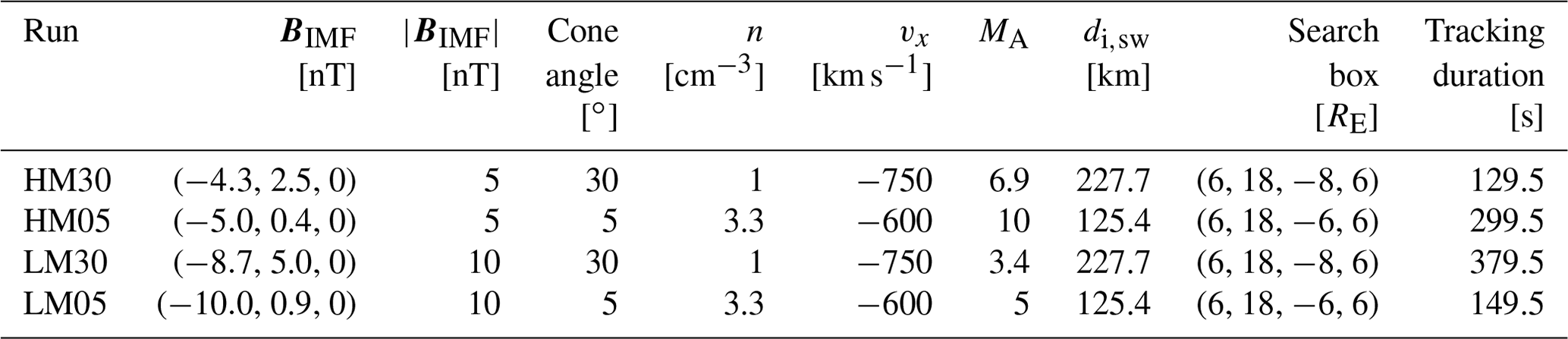
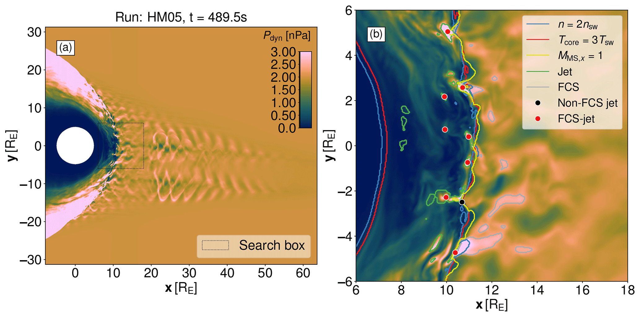
Figure 1 (a) Overview of dynamic pressure in the entire simulation box of run HM05 at an example time t=489.5 s. The dotted black box shows the extent of where we search for jets in this run. (b) Zoomed-in view of the search box at the same time in the same run. The plasma compression, plasma heating, and magnetosonic Mach number bow shock criteria are plotted as blue, red, and yellow contours respectively. Jets and FCS are delineated by green and grey contours respectively. Non-FCS jets and FCS jets are marked with black and red dots respectively.

2.2 Jet identification and tracking

In order to identify, separate, and track magnetosheath jets over time, we use the methods developed in Palmroth et al. (2021) and Suni et al. (2021). We search for jets in a search box which is chosen to focus on the subsolar magnetosheath in each run and for a tracking duration, limited by the simulation duration of each run, starting at 290 s (see Table 1). The extent of the search box in run HM05 is marked with dotted black lines in Fig. 1a. We define jets according to the criterion presented in Archer and Horbury (2013) as regions consisting of cells in the magnetosheath where the instantaneous dynamic pressure is at least twice the 3 min moving time average of the dynamic pressure, P_dyn≥2〈P_dyn〉_3min. Due to the limited simulation durations of the runs used in this study, we use a 3 min time average instead of the original 20 min time average used by Archer and Horbury (2013). The regions fulfilling this criterion at one time step in run HM05 are delineated with green contours in Fig. 1b. Jets that are identified at only one time step are discarded, as their propagation cannot be calculated from tracking the jet. While the method we use can identify jets anywhere in the magnetosheath, we additionally require that the jets we study form at the bow shock, as Palmroth et al. (2021) proposed that regions fulfilling the jet criteria that form deeper in the magnetosheath are merely momentary dynamic pressure fluctuations in a low ambient dynamic pressure environment rather than jets. We define the bow shock in two different ways adapted from Battarbee et al. (2020): the boundary where the temperature of the core ion population (as discussed in Wilson et al., 2014) is 3 times the solar wind temperature, T_core=3T_sw (plasma heating) and the boundary where the x directional magnetosonic Mach number is 1, $M_{\mathrm{ms},x}=v_x/\sqrt{v_{\mathrm{s}}^{\mathrm{2}}+v_{\mathrm{A}}^{\mathrm{2}}}=\mathrm{1}$ (red and yellow contours respectively in Fig. 1). A third definition, the boundary where the ion density is twice the solar wind density, n=2n_sw (plasma compression, blue contour in Fig. 1), is also shown for comparison, but because this threshold is often fulfilled within foreshock structures that contribute to shock reformation (Schwartz and Burgess, 1991; Johlander et al., 2022), it frequently misidentifies foreshock structures as magnetosheath plasma, and thus it is not used in jet categorisation or analysis. The magnetosheath is defined using the temperature criterion as the region of the simulation where T_core≥3T_sw. A jet is considered to form at the bow shock if the simulation cells in position space comprising the jet are in contact with either the temperature boundary or the Mach number boundary. Because we require information about whether magnetosheath jets are connected to foreshock structures or not, instantaneous values of T_core and M_MS,x are used instead of time averaging to acquire smooth and stable boundaries as done in e.g. Ng et al. (2022). The x directional Mach number is a suitable proxy for the bow shock location only near the nose of the bow shock, but as we search for jets in a subregion of the dayside magnetosheath (see Table 1), the behaviour of the x directional Mach number at the flanks is not an issue. We discard jets that exist for only a single simulation output time step, as well as jets that are found through visual inspection to clearly be the same structure as another jet in the data set or which form at a location that is found not to actually be at the bow shock.

The jets that form at the bow shock are initially separated into two categories as in Suni et al. (2021): those that form in contact with FCS, called FCS jets (marked with red dots in Fig. 1b) and those that do not, whose origins are unclear and which are called non-FCS jets (marked with a black dot in Fig. 1b). In Suni et al. (2021) we defined FCS as structures upstream of the bow shock (with the boundary defined as T_core=3T_sw) fulfilling the criteria of Eq. (1). In order to capture even the weakest FCS, in this study we use a magnetic threshold of η=1.1. The regions fulfilling the FCS criteria are delineated with grey contours in Fig. 1b).

3 Results

3.1 Jet classification

In order to study the propagation of jets in the magnetosheath, we define for each jet

• a formation time t₀ and

• a formation site (x₀,y₀),

where t₀ is the earliest simulation time step at which the jet is identified and, to emphasise the parts of the jet with higher dynamic pressure, (x₀,y₀) is a weighted mean of the cells comprising the jet,

$$\begin{array}{}\text{(2)}& \begin{array}{rl}(\stackrel{\mathrm{‾}}{x},\stackrel{\mathrm{‾}}{y})\left(t\right)& =\left({\displaystyle \frac{\sum _{k\in \mathrm{cells}\left(t\right)}{w}_k{x}_k}{\sum _{k\in \mathrm{cells}\left(t\right)}{w}_k}},{\displaystyle \frac{\sum _{k\in \mathrm{cells}\left(t\right)}{w}_k{y}_k}{\sum _{k\in \mathrm{cells}\left(t\right)}{w}_k}}\right)\\ w_k& ={\displaystyle \frac{P_{\mathrm{dyn},k}}{\langle P_{\mathrm{dyn},k}{\rangle }_{\mathrm{3}\min }}}-\mathrm{2},\end{array}\end{array}$$

at t₀, $(x_{\mathrm{0}},y_{\mathrm{0}})=(\stackrel{\mathrm{‾}}{x},\stackrel{\mathrm{‾}}{y})\left(t_{\mathrm{0}}\right)$, where the weights w_k are a measure of how much the dynamic pressure of each cell exceeds the criterion used to define the jets. To calculate the propagation velocity of the dynamic pressure enhancement associated with the jet, we define a formation of three virtual spacecraft (VSC) in an equilateral triangle centred on (x₀,y₀) and with an inter-spacecraft separation of $\sqrt{\mathrm{3}}\mathrm{d}x$, where dx=227 km is the position space resolution (cell size) of the simulation runs (see Table 1 caption), which gives $\sqrt{\mathrm{3}}\mathrm{d}x\approx \mathrm{393}$ km ≈ 0.06 R_E (see Fig. 2a). Assuming that the propagating structure can be considered a plane wave, we apply multi-spacecraft timing analysis (Paschmann and Daly, 1998; Schwartz, 1998) to the time series of dynamic pressure measured from t₀−10 s to t₀+10 s at each of the three VSCs. The dynamic pressure time series of the reference spacecraft, for which the VSC at $(x_{\mathrm{0}},y_{\mathrm{0}}+\mathrm{d}x)$ was chosen, is cross-correlated with the dynamic pressure time series of the other two VSCs, and the times of maximum cross-correlation are used to get time lags between the time series. Together with the VSC separations, this yields the propagation velocity v_n along the normal direction $\widehat{\mathit{n}}$ of the dynamic pressure enhancement corresponding to the jet. Because v_n does not take into account the plasma bulk velocity perpendicular to the normal direction $\widehat{\mathit{n}}$, we estimate the total propagation velocity of the jet in the simulation frame as $\mathit{v}={\mathit{v}}_{\mathrm{bulk}}+(v_n-{\mathit{v}}_{\mathrm{bulk}}\cdot \widehat{\mathit{n}})\widehat{\mathit{n}}$ (similarly to Archer et al., 2005), where v_bulk is the mean bulk velocity measured by the reference spacecraft in the [t₀−10 s, t₀+10 s] interval. Subintervals where the VSC is considered to be in the foreshock (defined as T_core<3T_sw), if any, are excluded.

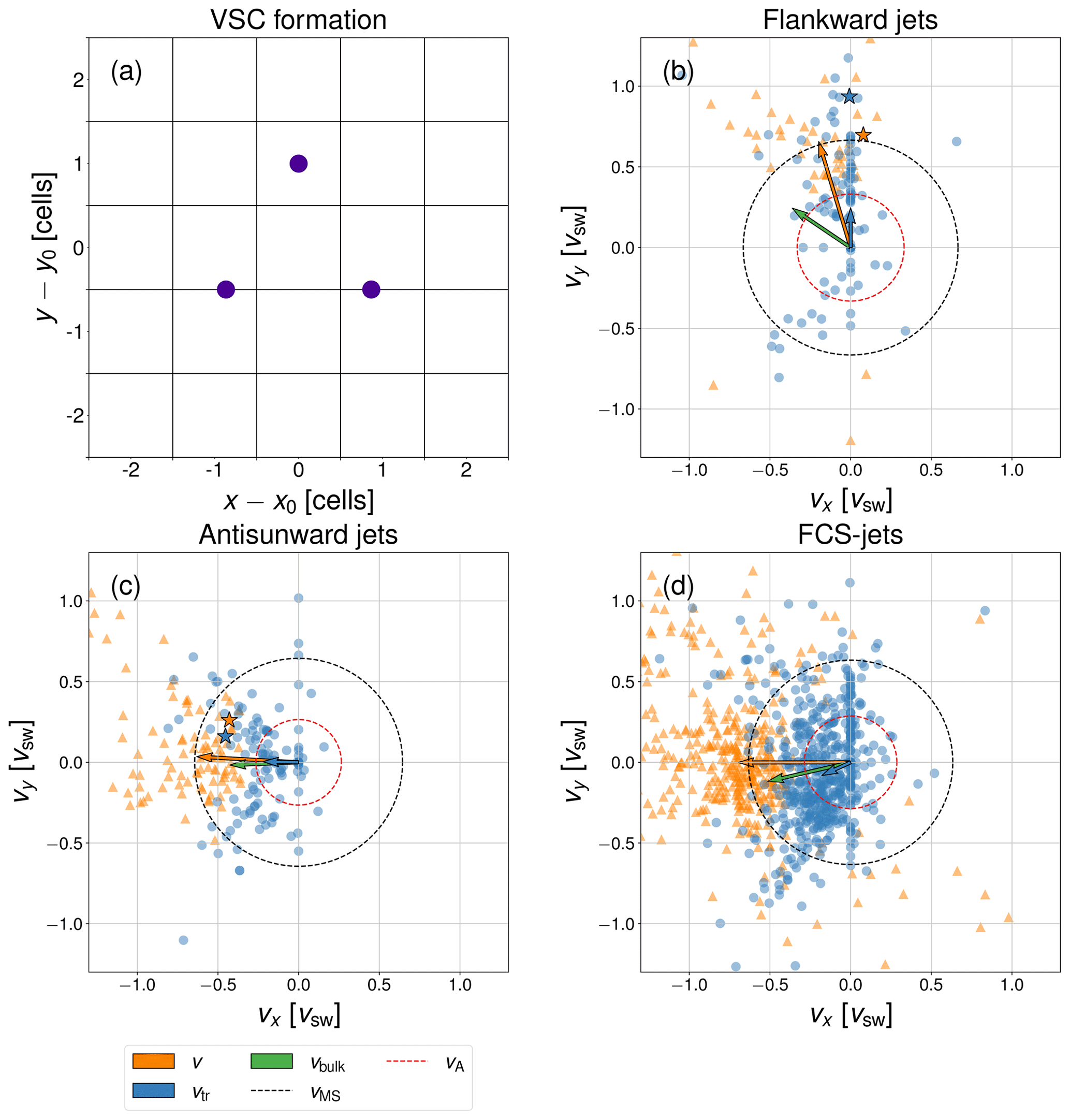
Figure 2 (a) Virtual spacecraft triangle formation, with respect to formation site (x₀,y₀), used in the timing analysis. (b–d) Jet propagation velocities in the simulation frame calculated from timing analysis (orange triangles) and based on the tracking of the weighted centres of the jets (blue dots), as well as median bulk velocity (green arrow) and median Alfvén (red circle) and magnetosonic speeds (black circle) for (b) flankward jets, (c) antisunward jets, and (d) FCS jets. Individual markers show the propagation velocity vectors of individual jets, while the arrows show the medians of each velocity. The stars mark the propagation velocities of example jets used in the case studies. Jet propagation velocities from timing analysis for which the maximum cross-correlation between any VSC pair is less than 0.8 are deemed unreliable and are not plotted or included in the calculations of the medians.

For each jet, we also use the time-evolution of $(\stackrel{\mathrm{‾}}{x},\stackrel{\mathrm{‾}}{y})$ to calculate an alternative propagation velocity v_tr, defined by the change of $(\stackrel{\mathrm{‾}}{x},\stackrel{\mathrm{‾}}{y})$ from t₀ to t₁:

$$\begin{array}{}\text{(3)}& {\mathit{v}}_{\mathrm{tr}}={\displaystyle \frac{(\stackrel{\mathrm{‾}}{x},\stackrel{\mathrm{‾}}{y})\left(t_{\mathrm{1}}\right)-(\stackrel{\mathrm{‾}}{x},\stackrel{\mathrm{‾}}{y})\left(t_{\mathrm{0}}\right)}{t_{\mathrm{1}}-t_{\mathrm{0}}}},\end{array}$$

where t₁ is taken 2 s (four output time steps at 0.5 s time resolution) after jet formation. If the jet only exists for less than 2 s, then t₁ is the last time when the jet is identified.

Because the calculation of v is based on the observation of a temporal structure by a small number of virtual spacecraft while the calculation of v_tr is based on the motion of a spatial structure consisting of cells in position space, it is expected that there will be some differences between the two estimates of the jet propagation velocity. For jets consisting of dynamic pressure enhancements that are large enough to be observed by all three VSCs and whose shapes do not change significantly during propagation, v and v_tr are expected to be quite similar. Because we do observe jets that are very small at the time of formation and then elongate in some direction, we expect there to be differences between v and v_tr in many cases.

Analysing the propagation velocities of non-FCS jets, we find that they can be classified based on whether they propagate antisunward or toward the flanks. Thus, we classify the non-FCS jets according to their directions of propagation in the simulation frame v: jets whose propagation velocity vector is within 45^∘ from the antisunward (−x) direction are classified as “antisunward jets”, while the remaining jets are classified as “flankward jets”. In cases when the maximum cross-correlation of the dynamic pressure time series between any VSC pair is less than 0.8 (Eastwood et al., 2005a), we deem the timing analysis as being possibly unreliable and perform the classification based on v_tr instead. This can occur when not all virtual spacecraft observe the jet-associated dynamic pressure enhancement clearly. After the non-FCS jets are categorised in this way, the formation sites and times of the jets are visually inspected and jets that are not actually connected with the bow shock (as defined by the core heating or magnetosonic Mach number criteria) or which are clearly part of the same structure as any previously identified jet are discarded. Table 2 shows the number of jets of each category found in each of the four simulation runs, as well as the number of FCS jets for comparison and the ratios of the numbers of antisunward, flankward, total non-FCS jets, and FCS jets to the total number of all jets. FCS jets make up 71 % of all jets. Because we discard jets that exist for only one time step in this study, and because the previous estimate of 75 % found by Suni et al. (2021) was based on a figure, there is a slight difference between this study and Suni et al. (2021). Non-FCS jets make up the remaining 29 % of jets, and roughly half of the non-FCS jets are antisunward and half flankward. The ratio of antisunward jets to flankward jets is >1 for the 5^∘ IMF cone angle runs, and <1 for the 30^∘ cone angle runs.

Table 2 Number of jets of each category and total number of non-FCS jets found in each of the different simulation runs as well as in all runs combined. The number of FCS jets found in each run and all runs combined are also given, as well as the proportions of the different jet categories and FCS jets to the total number of jets.

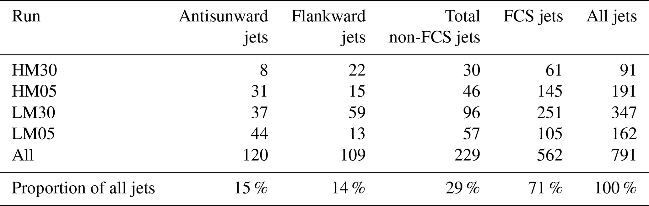
Figure 2b–d shows the propagation velocities v and v_tr for all flankward jets, antisunward jets, and FCS jets respectively, as well as the medians of the propagation velocities and average bulk velocity at the reference VSC, with the median Alfvén and magnetosonic speeds at the reference VSC for comparison. v obtained from timing analysis where the maximum cross-correlation between any VSC pair is below 0.8 are not plotted or included in median calculations. The v_x and v_y axes are both cropped to $[-\mathrm{1.3}{v}_{\mathrm{sw}},\mathrm{1.3}{v}_{\mathrm{sw}}]$ as this allows the majority of the data points to be shown without obscuring the medians and Alfvén and magnetosonic speeds. Here, 6 flankward jet, 8 antisunward jet, and 58 FCS jet v data points fall outside the axes limits, while 0, 1, and 20 flankward, antisunward and FCS jet v_tr data points fall outside the axes. We can see that in the case of flankward jets, propagation is biased toward the dusk flank, as is the bulk flow, which suggests that most flankward jets form on the duskward side of the subsolar point. For antisunward jets and FCS jets, on the other hand, the propagation velocities and bulk flow are distributed almost equally on the dawn and dusk sides, while the bulk flow is slightly biased toward dawn for FCS jets. This is consistent with the deflection of the antisunward solar wind flow by the shock around the subsolar point. Most flankward jets propagate faster flankward than the bulk flow, while the propagation of antisunward jets appears to be quite closely aligned with the bulk flow. For all jet types, we can see some cases where v_tr has no x directional component. This is likely due to those particular jets being very short-lived and extending only one cell in the x direction, in which case the weighted centre coordinate is effectively quantised due to the finite simulation cell size. Indeed, 12 % of flankward jets, 5 % of antisunward jets, and 2 % of FCS jets have a lifetime maximum size of only one cell, but excluding these jets does not change the results of the analyses conducted in this study.

3.2 Case studies

Having classified the non-FCS jets, we investigate possible differences in the plasma and magnetic field properties surrounding the formation of jets of different categories by selecting one typical flankward jet (marked with stars in Fig. 2b) and one typical antisunward jet (marked with stars in Fig. 2c) as examples for individual analysis. Figure 3 shows the properties surrounding the formation of the example flankward jet: panel (a) shows the dynamic pressure around the formation site (marked by the crosshairs) at t₀, with contours delineating regions where the different bow shock criteria and the jet and FCS criteria are fulfilled. The black dot marks the weighted centre $(\stackrel{\mathrm{‾}}{x},\stackrel{\mathrm{‾}}{y})$ of the flankward jet in question. The streamlines show the magnetic field. Panel (b) shows the time series from t₀−10 s to t₀+10 s of dynamic pressure along a line segment centred on (x₀,y₀) and extending 20 cells (∼0.71 R_E) in the −x and +x directions. Also shown are contours marking the x coordinates of the three bow shock criteria at y₀ as a function of time, as well as crosshairs marking (x₀,t₀). Panel (c) shows the results of the timing analysis for the flankward jet under consideration. Panels (d)–(h) show the time series from t₀−10 s to t₀+10 s at the formation site of density; velocity x component, magnitude of the yz components, and the total magnitude; dynamic pressure; magnitude of the magnetic field x component, yz components, and the total field; and temperature components perpendicular and parallel to the magnetic field. The decision to show yz components instead of y and z separately was made to highlight the difference between the antisunward component and its orthogonal counterpart, as the magnetosheath flow and the effect of IMF clock angle on the magnetosheath are expected to be roughly rotationally symmetric. To improve clarity, we plot $\left|B_x\right|$ instead of B_x as the sign of B_x is mainly determined by the sign of the IMF B_x. The dashed lines mark t₀.

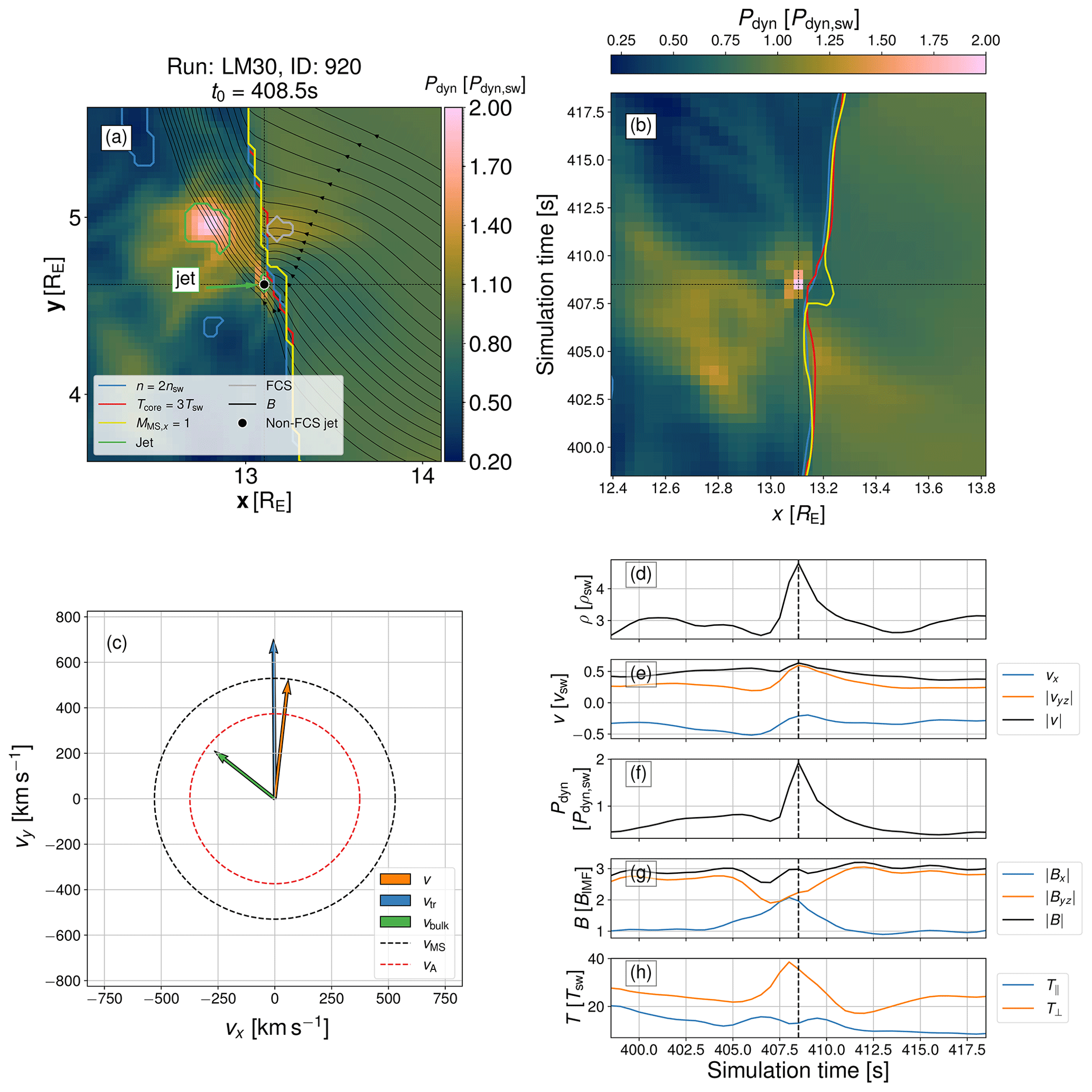
Figure 3 Properties of the near-bow shock environment around the formation time t₀ and place (x₀,y₀) of an example flankward jet: (a) view of dynamic pressure with contours showing the fulfilling of the three bow shock criteria (plasma compression in blue plasma heating in red and magnetosonic Mach number in yellow), the jet criteria (green), and FCS criteria (grey), with black dots indicating the weighted centres of tracked non-FCS jets, and magnetic field lines shown as black streamlines; (b) cut-through time series around t₀ and x₀ at y₀ showing dynamic pressure and the three bow shock criteria as contours; (c) timing analysis from a triangle of VSCs centred on (x₀,y₀), showing propagation velocities, bulk velocity, and Alfvén and magnetosonic speeds; (d–h) time series of plasma and magnetic field properties around t₀ at (x₀,y₀).

We can see from the simulation view (Fig. 3a) that the jet forms at the bow shock several R_E duskward of the subsolar point and that while waves are visible in the magnetic field on the upstream side, the dynamic pressure sunward of the jet is quite homogeneous, indicating the absence of compressional waves. This suggests that the formation site is close to the ULF foreshock edge. Immediately sunward of the formation site, the three bow shock criteria are not exactly co-located – the magnetosonic Mach boundary is sunward of the other two – i.e. the bow shock is “non-local” (Battarbee et al., 2020). The cut-through time series shows that the formation of the jet is associated with lower dynamic pressure upstream of the formation site. Just before the formation time, the appearance of the bow shock non-locality can be seen. Figure 3c shows that the magnetosheath bulk velocity is sub-Alfvénic, while the jet propagation velocities are all super-Alfvénic in the simulation frame. The weighted centre of the jet even propagates with supermagnetosonic speed. The time series show that the formation of the jet is associated with a large and steep increase in plasma density, as well as deflection of the plasma flow from v_x-dominated to v_yz-dominated. The formation is also preceded by a strengthening of B_x and weakening of B_yz. Just before the formation time, there is a large increase in T_⟂ and a small decrease in T_∥, and as a consequence the temperature anisotropy $T_{⟂}/T_{\parallel }$ increases.

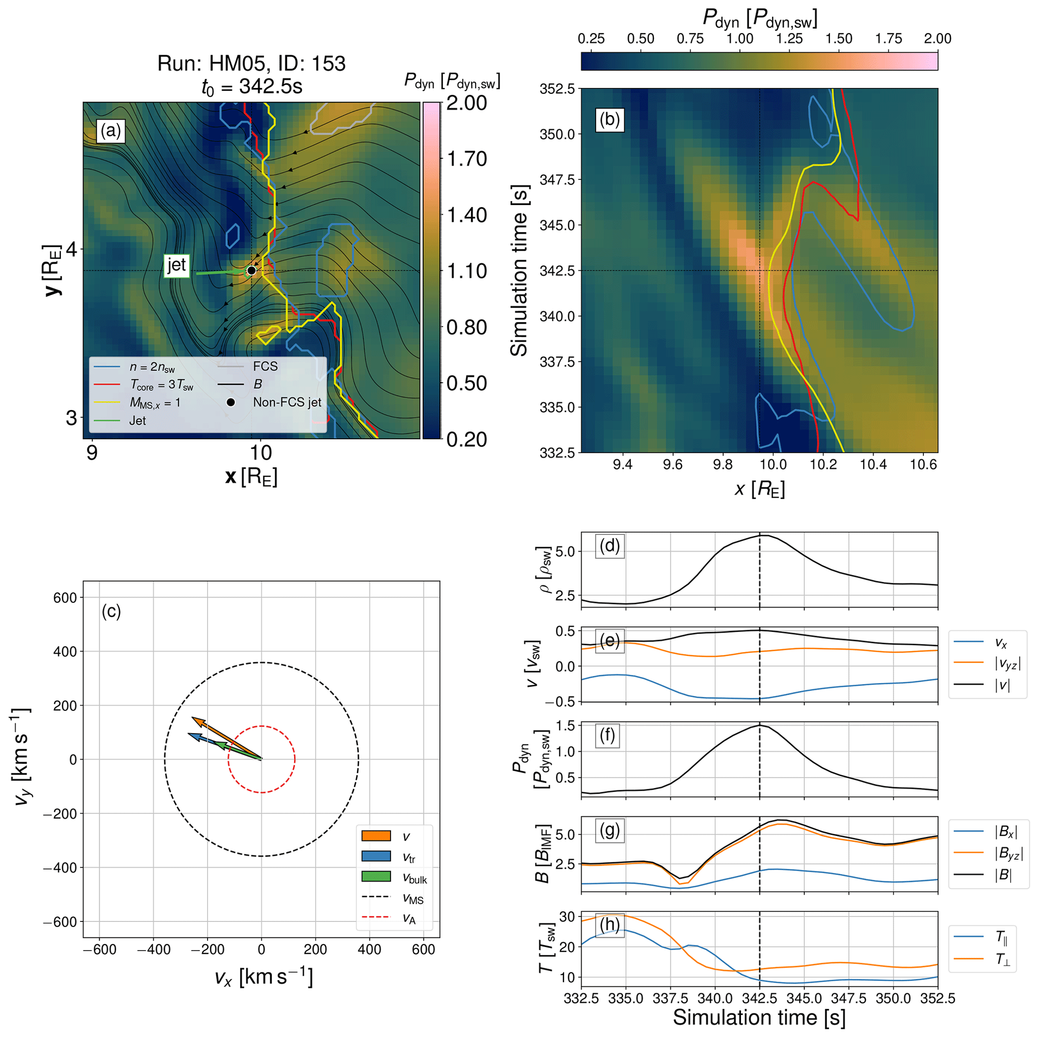
Figure 4 shows the surroundings of the forming example antisunward jet, presented in the same way as the example of the flankward jet. The simulation view in panel (a) shows that this antisunward jet also forms several R_E duskward of the subsolar point but under very different conditions. As the simulation run in question has an IMF cone angle of 5^∘, the formation site is downstream of the deep ULF foreshock. The magnetic field both upstream and downstream displays intense fluctuations, and compressional structures can be seen on the upstream side. The bow shock immediately sunward of this jet is also non-local, but now the magnetosonic Mach number boundary is earthward of the other two bow shock boundaries. In the cut-through time series, we can see a foreshock dynamic pressure enhancement advecting toward and impacting the bow shock, which is followed by the formation of the jet at the impact location. A few seconds after the formation time, a bow shock reformation event (see Johlander et al., 2022) occurs, as shown by the blue contour extending further into the upstream in Fig. 4b. The timing analysis shows that the jet propagation velocities and ambient bulk velocity are all super-Alfvénic but submagnetosonic, and the jet propagates in the bulk flow direction. The time series show that the formation of the jet is associated with an increase in density and magnetic field strength, to which the B_yz component contributes more than B_x. The formation is preceded by enhanced v_x and a decrease in v_yz as well as a decrease in both T_⟂ and T_∥ and approximately isotropic temperature.

Figure 4 Same format as Fig. 3 but for an example antisunward jet.

3.3 Statistical analysis

The examples show that flankward and antisunward jets appear to differ in the properties of the plasma surrounding and comprising them. To investigate this further, we conduct a statistical study of all flankward, antisunward, and FCS jets. Figure 5 shows a superposed epoch analysis (SEA) of cut-through time series of plasma density (panels a, f, k), v_x (panels b, g, l), dynamic pressure (panels c, h, m), magnetic field strength (panels d, i, n), and temperature (panels e, j, o), with t₀ of each jet serving as the epoch time and x₀ serving as the epoch x. Also shown are the average bow shock distances at y₀ as a function of time. We can see that, on average, flankward jets are not associated with any foreshock structures convecting into the bow shock, at least not exactly sunward of the formation sites. Flankward jets also appear to be mainly density driven, with little-to-no velocity enhancement in the magnetosheath at the formation site and time but a noticeable enhancement of density. The plasma at the formation site and time is generally cooler than the ambient magnetosheath plasma but is surrounded by localised temperature enhancements. Flankward jets are associated with a sunward motion of the bow shock, with the motion becoming faster after the formation time. The jet formation is also followed by an enhancement of magnetic field strength in the magnetosheath. Antisunward and FCS jets, on the other hand, appear to be very similar to each other and different from flankward jets. Both are associated with foreshock structures of enhanced density, dynamic pressure, and magnetic field advecting into the bow shock. The impact is concurrent with jet formation and the incursion of fast and cold solar wind plasma into the magnetosheath. For all jet types shown in Fig. 5, the bow shock location changes over time. The sunward motion occurring over the entire 30 s time window is most likely due to 2D simulation effects which cause the bow shock to move sunward in general, while the short timescale changes around the jet formation times could be local corrugation of the bow shock.

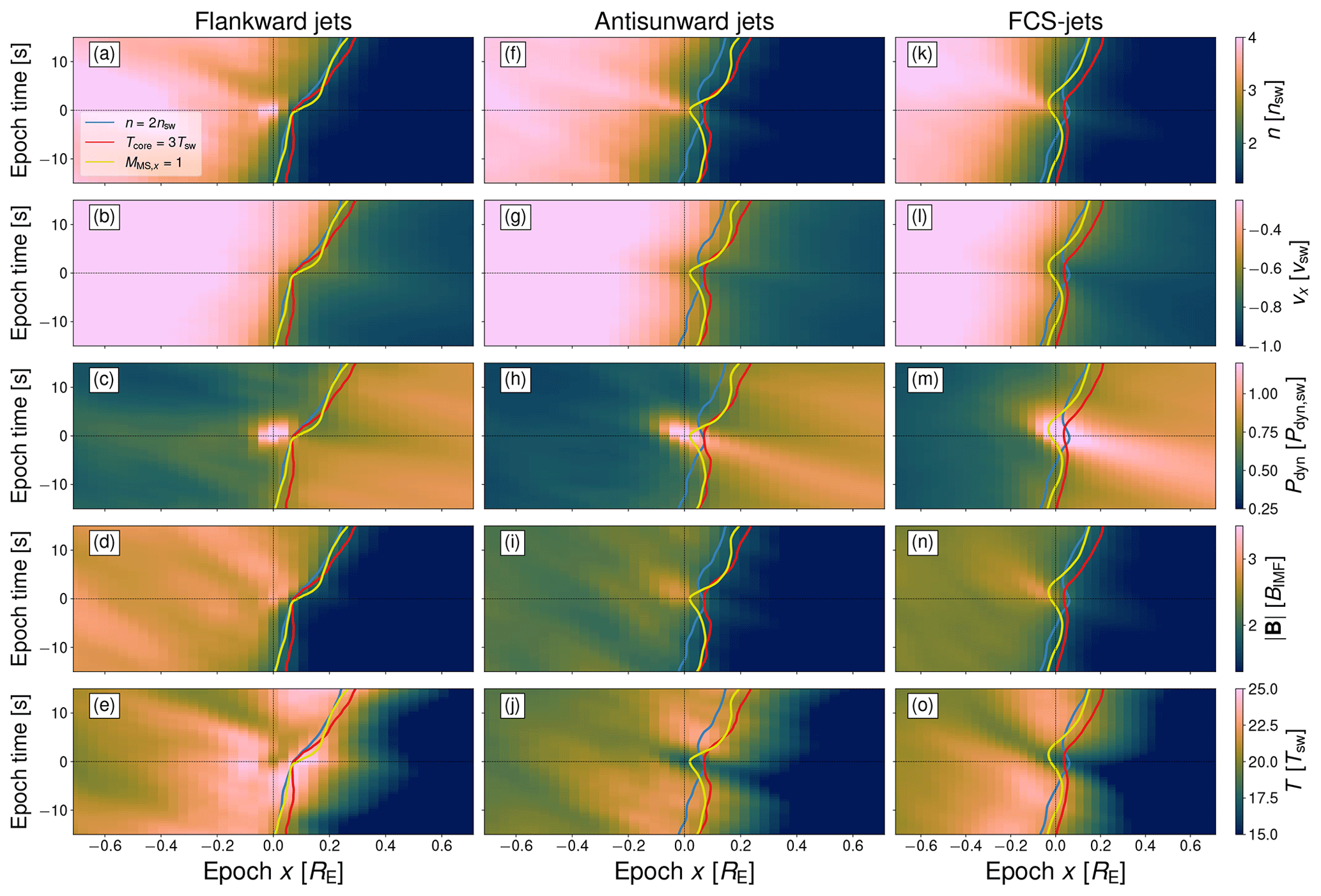
Figure 5 Superposed epoch analysis of cut-through time series of plasma density, x directional velocity component, dynamic pressure, magnetic field strength, and temperature for flankward jets, antisunward jets, and FCS jets. The formation time t₀ for each jet was chosen as the epoch time, while the formation site x coordinate x₀ was chosen as the epoch location. Also shown are the average locations of the plasma density, plasma heating, and magnetosonic Mach number bow shock criteria as blue, red, and yellow contours respectively.

Figure 6 shows an SEA of the time series at the jet formation sites of plasma density (panels a, g, m), velocity components and magnitude (panels b, h, n), dynamic pressure (panels c, i, o), magnitude of magnetic field components and total field (panels d, j, p), parallel and perpendicular temperature (panels e, k, q), and temperature anisotropy (panels f, l, r) for flankward jets, antisunward jets, and FCS jets. The formation time of each jet is chosen as the epoch time. Also shown are box-and-whisker plots showing the median, 25th percentile, 75th percentile, and the lowest and highest data points that are within 1.5 times the interquartile range (IQR) from the quartiles of the time series data used in the SEA sampled at epoch times −6.5, 0, and 6.5 s. We can see that flankward jets exhibit the greatest density enhancement on average, while FCS jets exhibit the smallest. To some extent, this may be affected by the fact that most jets of all kinds are found in runs LM05 and LM30 (see Table 2), where the low solar wind Alfvén Mach number may lead to less compression of the plasma at the shock. In contrast, FCS jets display the greatest enhancement in velocity, while flankward jets display the smallest. For flankward jets the velocity enhancement is in the v_yz component, unlike for antisunward and FCS jets, where both v_x and v_yz are enhanced. The resulting enhancement in dynamic pressure is similar for all kinds of jets. The magnetic field enhancement is also similar across all categories, with the main difference being an enhancement in B_yz after jet formation for flankward jets. The formation of all kinds of jets is preceded by and associated with a decrease in T_∥, but for flankward jets formation is associated with nearly constant T_⟂ that leads to enhanced temperature anisotropy, whereas for antisunward and FCS jets T_⟂ also decreases around the formation time. The box-and-whisker plots show that there is considerable variation in the time series of jets belonging to each category, but the interquartile ranges are similar to the differences between the categories.

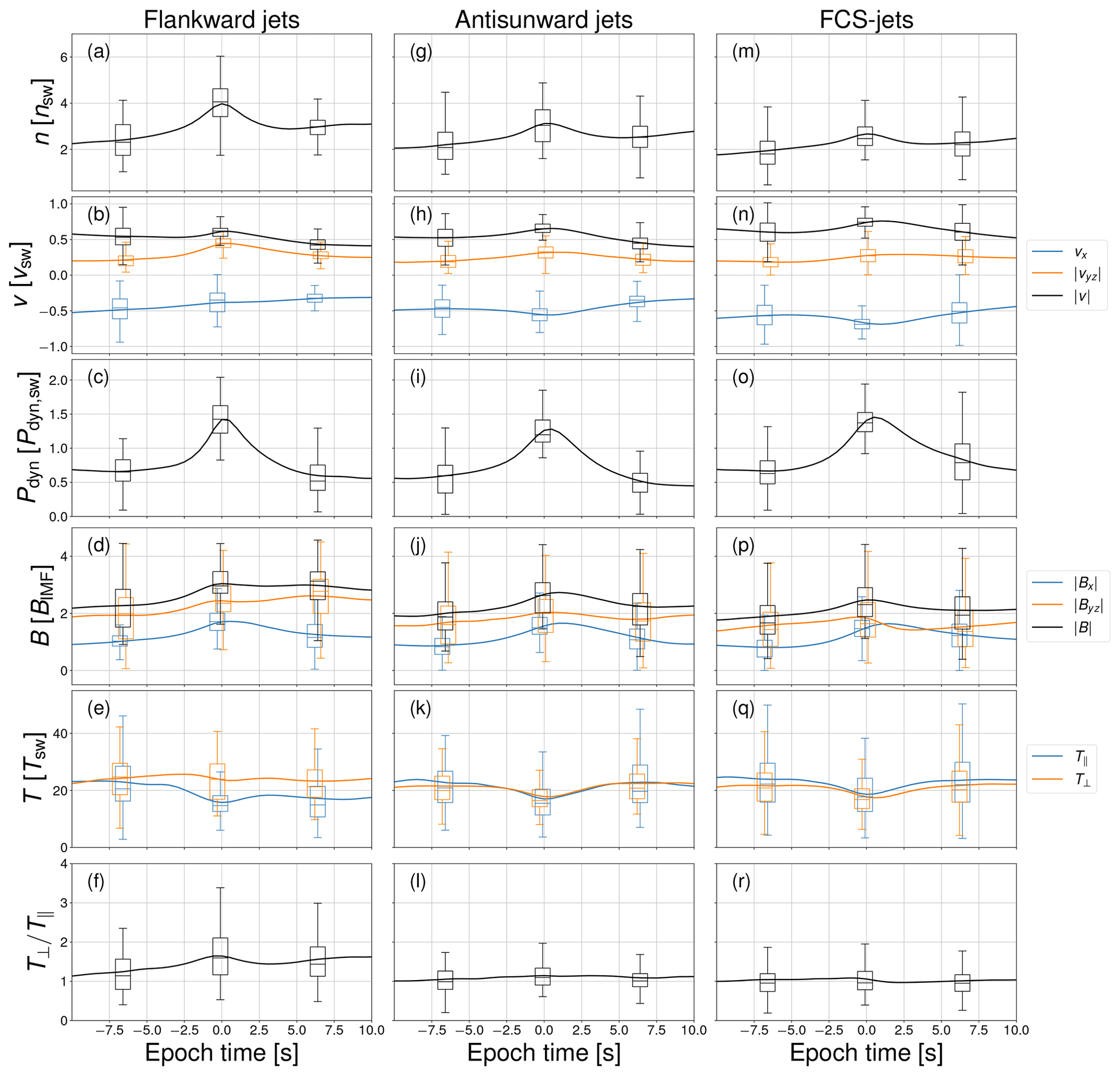
Figure 6 Superposed epoch analysis of single VSC time series, showing density, velocity components and magnitude, dynamic pressure, magnetic field components and magnitude, parallel and perpendicular temperature, and temperature anisotropy for flankward jets, antisunward jets, and FCS jets. The formation time t₀ of each jet was chosen as the epoch time. Also shown are box-and-whisker plots at epoch times −6.5, 0, and 6.5 s. The boxes show the 25th percentile, the median, and the 75th percentile, while the whiskers mark the lowest and highest data points that are within 1.5 times the interquartile range ($\mathrm{IQR}=Q_{\mathrm{3}}-Q_{\mathrm{1}}$) from the quartiles.

Finally, we investigate the formation sites of the different jet categories. Figure 7 shows the formation sites of flankward jets and antisunward jets, as well as FCS jets for comparison, in the four simulation runs. Also depicted are the extent of the ion foreshock, defined as the presence of reflected ions (dashed black curve visible in panels b and d), the extent of the ULF foreshock, defined as enhancement of B_z, at t=400 s in each run, similarly to Turc et al. (2018) (pink and brown contours), and the extent of the jet search box (dotted black lines; see Table 1) in each run. The example jets studied in Sect. 3.2 are marked with stars. We can see that antisunward and FCS jets form everywhere at the bow shock in the search box in all simulation runs, but the majority of flankward jets form at the edge of the ULF foreshock on the dusk flank side, in agreement with the median bulk velocity in Fig. 2b, in the 30^∘ IMF cone angle runs.

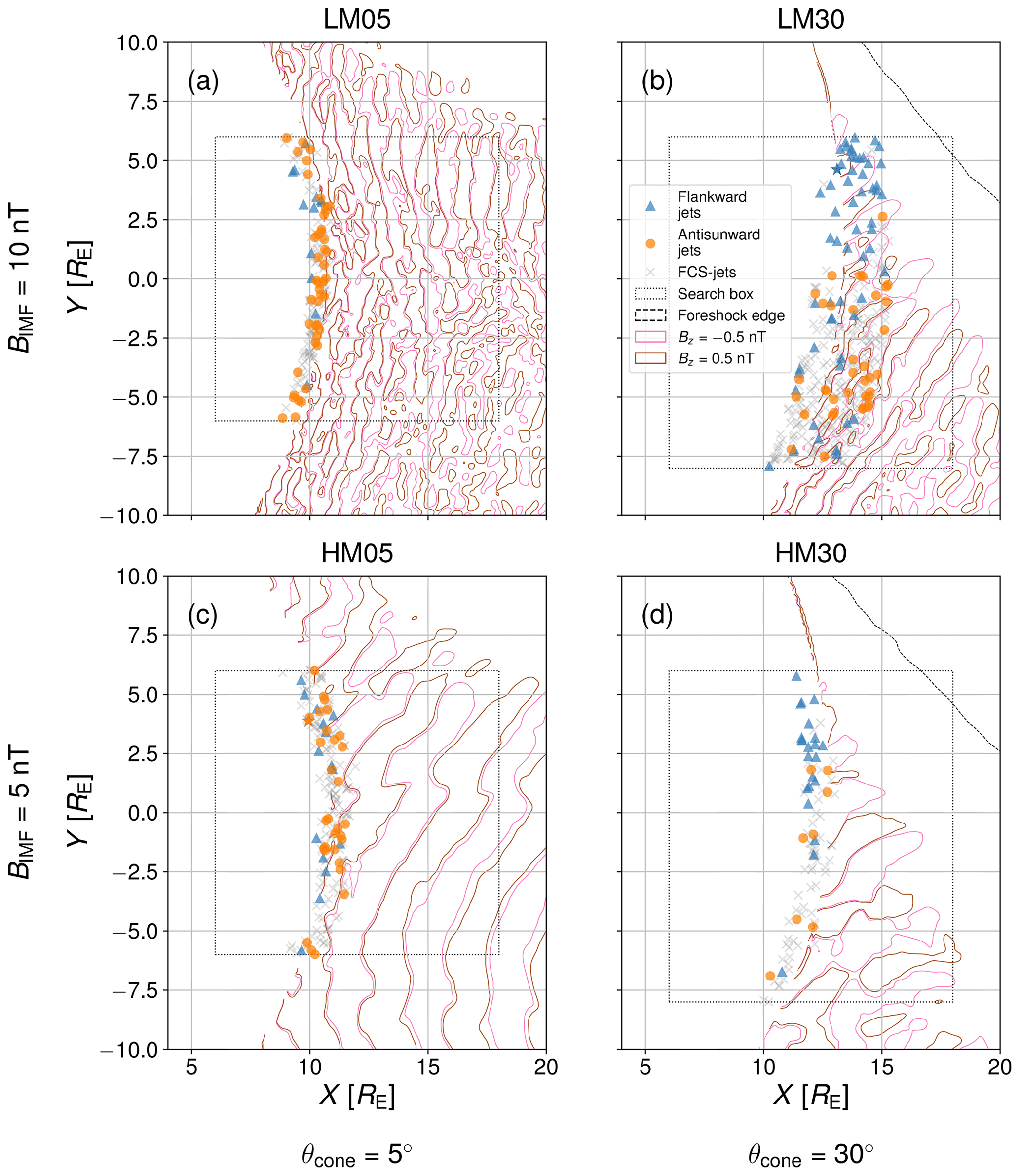
Figure 7 Formation sites (x₀,y₀) of all non-FCS jets separated by category, as well as FCS jets for comparison, in the four runs: (a) LM05, (b) LM30, (c) HM05, and (d) HM30. Flankward and antisunward jets are shown as blue triangles and orange circles respectively. The actual spatial extent of the jets is not shown. The jets used for the case studies are marked with stars. FCS jets are shown as grey crosses. The dashed black curve shows the edge of the foreshock, as defined by the presence of reflected ions, and thus the extent of the ion foreshock at t=400 s in each run. The pink and brown curves show, also at t=400 s, the contours of $B_z=-\mathrm{0.5}$ nT and B_z=0.5 nT respectively, indicating the presence of ULF waves and the extent of the ULF foreshock. The horizontal dotted black lines show the extent of the jet search box in each run.

4 Discussion

In this study we have investigated the formation of jets that were not associated with foreshock compressive structures in Suni et al. (2021) by classifying them based on their direction of propagation. We have found that these non-FCS jets can be separated into two categories based on their direction of propagation: flankward and antisunward jets. We have conducted case studies by analysing two example jets in four different ways: 2D simulation views, cut-through time series, analysis of jet propagation, and virtual spacecraft time series at the formation site. We have performed a statistical analysis by conducting superposed epoch analyses of the cut-through time series and the virtual spacecraft time series, as well as compared the median propagation velocities and visualised where along the bow shock different jets form, for flankward jets and antisunward jets, as well as for FCS jets for comparison. We have found that antisunward jets have the same properties and origin as FCS jets. Flankward jets, on the other hand, differ in many ways from the other jets.

As we have seen in Fig. 5, antisunward jets and FCS jets are both associated with foreshock structures of enhanced density, dynamic pressure, and slightly enhanced magnetic field strength convecting into the bow shock, the impact coinciding with jet formation in the magnetosheath. The impact is also associated with the intrusion of fast and cold solar wind plasma into the magnetosheath. We find that the plasma in the jets is colder and faster than the surrounding plasma, which agrees with previous results from Vlasiator and MMS spacecraft observations (Palmroth et al., 2021) as well as data from the five Time History of Events and Macroscale Interactions during Substorms (THEMIS) spacecraft (Plaschke et al., 2013). From Fig. 6 we have seen that the velocity enhancement at the jet formation site is mainly in v_x, the magnetic field enhancement is mainly in B_x, and the temperature decrease is both in the parallel and the perpendicular component, for both antisunward and FCS jets. Figures 2 and 7 show that antisunward and FCS jets form in the same regions of the magnetosheath and they both mainly propagate antisunward.

Our analysis of the antisunward jets thus indicates that antisunward jets were previously categorised in the non-FCS group due to the selected thresholds for the parameter η and/or the dynamic pressure threshold 1.2 in Eq. (1), and not because they are a fundamentally different phenomenon. Because antisunward and FCS jets make up 683 of the total 790 jets used in this study (see Table 2), this means that 86 % of jets that form at the bow shock under the steady solar wind conditions and quasi-radial IMF in our four simulation runs are associated with structures of enhanced dynamic pressure and magnetic field strength in the foreshock. As can be seen in Fig. 5, as the foreshock structures approach the bow shock, their density/dynamic pressure and magnetic field grow. This agrees with the formation mechanism of Raptis et al. (2022b), who used the MMS spacecraft constellation to observe foreshock waves becoming compressive when approaching the bow shock and subsequently causing bow shock reformation and magnetosheath jet formation as they make contact with the shock. While the average density and magnetic field in Fig. 5 do not quite reach magnetosheath values and thus systematic bow shock reformation is not visible, the steepening process of the structures/waves is similar. It should be noted, however, that the agreement between this study and Raptis et al. (2022b) does not exclude the possibility that the ripple formation mechanism proposed by Hietala et al. (2009) or the magnetokinetic mechanism of Omelchenko et al. (2021) are also responsible for, or linked to, the formation of jets under similar or different solar wind conditions. However, we have not found these mechanisms at work in our simulations so far.

In contrast, the flankward jets that make up the remaining 14 % of the jets investigated in this study have different properties. Their large temperature anisotropy (with T_⟂ being larger than T_∥; see Fig. 6) and the deflection of the shocked solar wind plasma (enhancement of v_yz rather than v_x) are reminiscent of the “quasi-perpendicular jets” described by Raptis et al. (2020). However, these quasi-perpendicular jets in Raptis et al. (2020) show modest enhancements or even decreases in the plasma density, while the flankward jets in this study are on average associated with higher density enhancements than antisunward and FCS jets. The unexpectedly large overall density found in flankward jets could be due to the 2D nature of the simulation runs used in this study, as this prevents structures from dissipating in the out-of-plane direction (Pfau-Kempf et al., 2016; Suni et al., 2021), although this cannot account for the temporary enhancement in density. The observation that some jets are more density driven than others is, however, consistent with spacecraft measurements (Archer and Horbury, 2013), and these could be related to the plasmoids of Karlsson et al. (2015). From Fig. 6 we can also see that the temperature anisotropy at the formation site remains greater than 1 for up to 10 s after jet formation, as does the enhancement of B_yz.

Our analysis of the flankward jets therefore suggests that the formation of flankward jets could be concurrent with a local change in bow shock geometry from quasi-parallel to quasi-perpendicular. Quasi-perpendicular shocks are associated with a sharper jump of plasma and magnetic field properties across the shock than quasi-parallel shocks, which could explain the enhancement of density inside the flankward jets. The enhancement of v_yz and decrease in v_x are also consistent with a change in the angle between the bow shock normal and the direction of the incoming solar wind. The local turning of a shock from quasi-parallel to quasi-perpendicular due to growing out-of-plane magnetic perturbations is a known phenomenon (e.g. Baumjohann and Treumann, 1996), but this turning has also been observed in association with bow shock reformation (Gingell et al., 2017; Liu et al., 2021). Liu et al. (2021) find that this turning can occur due to reformation at the oblique bow shock, which could explain why flankward jets form mainly at the edge of the ULF foreshock upstream of the oblique bow shock. At the oblique shock, the ULF waves are able to modulate the upstream conditions but do not generate compressional structures that would lead to the formation of antisunward or FCS jets instead.

Considering the fact that the velocity enhancements of flankward jets are in the y direction and that they are associated with weakening v_x (see Fig. 6), it should be noted that these jets would not necessarily be captured if we had used a different jet criterion. For instance, the Plaschke et al. (2013) and Koller et al. (2022) criteria consider only x directional dynamic pressure, which may not be enhanced in flankward jets. Furthermore, Raptis et al. (2022a) showed that the velocity distributions inside of magnetosheath jets can consist of multiple particle populations – a faster jet population and a slower background population, in which case using criteria that rely on plasma moments and derived properties, such as dynamic pressure, may not correctly identify all jets. The implications of this in Vlasiator will be investigated in a future study.

5 Conclusions

In this study we have investigated the origins of magnetosheath jets in four two-dimensional simulation runs of the global magnetospheric hybrid-Vlasov model Vlasiator. We have focused on jets that Suni et al. (2021) found not to be associated with foreshock compressive structures (FCS). We have found that these jets can be separated based on propagation direction, either antisunward or flankward. We have shown that the FCS-associated jets previously investigated in Suni et al. (2021) and the antisunward jets investigated in this study are fundamentally the same, and thus 86 % of all the jets forming at the bow shock in four Vlasiator simulation runs with steady solar wind conditions and quasi-radial IMF form due to foreshock structures of enhanced dynamic pressure and magnetic field strength impacting the bow shock. Thus the reason why the antisunward jets were previously categorised in the non-FCS group is because the defining criteria of FCS jets were too restrictive. The formation of these jets in the simulations is consistent with the formation mechanism observed with spacecraft in Raptis et al. (2022b).

We show that the remaining 14 % of jets (the flankward jets) exhibit different properties from the 86 % of jets that are associated with foreshock compressive structures. The flankward jets are not associated with foreshock structures and form mainly downstream of the ULF foreshock boundary. Instead, they display some features of quasi-perpendicular magnetosheath plasma, such as high temperature anisotropy and enhanced magnetic field and velocity in the direction transverse to the shock front. The flankward jets also have enhanced density, and in this respect they differ from spacecraft observations of jets in the quasi-perpendicular magnetosheath. These properties indicate that they might form behind a part of the bow shock that locally changes from quasi-parallel to quasi-perpendicular. If this is true, multi-spacecraft measurements should be searched for simultaneous observations of magnetosheath jets and signatures of the bow shock turning from quasi-parallel to quasi-perpendicular, such as disappearance of reflected ions just upstream of the shock. While jets that propagate flankward are not expected to have direct effects on the magnetosphere by impacting the magnetopause, these results advance our understanding of the effects that bow shock reformation can have in the magnetosheath.

To our knowledge, there are no observational studies characterising the propagation velocity of magnetosheath jets to which we could directly compare our results. This is likely due to the challenges in obtaining the jet propagation velocity, which requires multi-point measurements. Future studies could for example revisit observations of magnetosheath jets from the four-spacecraft MMS mission to test whether observed jets can be categorised based on their propagation direction. Based on this study it would be also be important to search spacecraft observations for evidence of the local turning of the bow shock from quasi-parallel to quasi-perpendicular.