Three-dimensional ionospheric conductivity associated with pulsating auroral patches: reconstruction from ground-based optical observations

Pulsating auroras (PsAs) appear over a wide area within the aurora oval in the midnight–morning–noon sector. In previous studies, observations by magnetometers on board satellites have reported the presence of field-aligned currents (FACs) near the edges and interiors of pulsating aurora patches. PsAs are thus a key research target for understanding the magnetosphere–ionosphere coupling process. However, the three-dimensional (3-D) structure of the electric currents has yet to be clarified, since each satellite observation is limited to a single dimension along its orbit. This study's aim was a reconstruction of the 3-D structure of ionospheric conductivity, which is necessary to elucidate the 3-D ionospheric current. Tomographic analysis was used to estimate the 3-D ionospheric conductivity for rapidly changing auroral phenomena such as PsAs. The reconstructed Hall conductivity reached its maximum value of 1.4 × 10⁻³ S m⁻¹ at 94 km altitude, while the Pedersen conductivity reached its maximum value of 2.6 × 10⁻⁴ S m⁻¹ at 116 km altitude. A secondary peak in the Pedersen conductivity, due to electron motion, at 9.9 × 10⁻⁵ S m⁻¹ appears at 86 km altitude. The electron Pedersen conductivity maximum value in the D region was approximately 38 % of the ion Pedersen conductivity maximum value in the E region. The FAC, derived under the assumption of a uniform ionospheric electric field, was approximately 70 µA m⁻² near the edge of the PsA patch. This FAC value was approximately 10 times that observed by satellites in previous studies. If the conductivity around the patch is underestimated or the assumption of a uniform field distribution is incorrect, the FAC could be overestimated. By contrast, due to sharper boundary structures, the FAC could actually have had such a large FAC.

1 Introduction

Pulsating auroras (PsAs) are a kind of diffuse aurora with a quasi-periodic luminosity modulation of ∼ 2–20 s (Yamamoto, 1988). Although PsAs are dimmer in brightness than typical discrete auroras (some hundreds of Rayleigh (R) to tens of kilo-Rayleigh at atomic oxygen (OI) 557.7 nm; a few hundred Rayleigh to ∼ 10 kR at the N${}_{\mathrm{2}}^{+}$ first negative band 427.8 nm) (McEwen et al., 1981; Royrvik and Davis, 1977), they are a general auroral phenomenon because of their wide range of appearances from the midnight to noon sectors depending on geomagnetic activities (Oguti et al., 1981; Royrvik and Davis, 1977). Typically, PsAs are grouped into three classes: auroral arcs, arc segments, and patches. This study focuses on patch-type PsAs.

Previous observations by satellite-borne magnetometers have indicated the occurrence of field-aligned currents (FACs) associated with PsA patches (Fujii et al., 1985; Gillies et al., 2015). Pairs of FACs flowing into and out of PsA patch edges are thought to be closed via the Pedersen current flowing within the PsA patch in the direction perpendicular to the geomagnetic field (Fujii et al., 1985; Oguti et al., 1984). PsAs are caused by precipitating electrons from a few kilo-electronvolt (keV) to tens of keV scattered into the loss cone by whistler-mode chorus waves excited near the magnetic equator (Kasahara et al., 2018; Nishimura et al., 2010, 2011). Chorus waves, which propagate to the off-equator, scatter high-energy electrons from tens of keV to a few mega-electronvolt (MeV) and enhance the electron density in the ionospheric D region (Kawamura et al., 2021; Miyoshi et al., 2010, 2015, 2020, 2021; Shumko et al., 2021). Hosokawa and Ogawa (2010) investigated the altitude profile of the electron density obtained with the European Incoherent Scatter (EISCAT) radar, reporting that the Pedersen current carried by electrons was seen in the D region (at approximately 80–95 km altitudes) associated with PsAs in addition to the commonly seen ion Pedersen current in the E region (at an altitude of 120 km). They suggested that the electron Pedersen current in the D region contributed to FAC closure in the ionosphere because the PsA emission altitude was closer to the peak altitude of the electron Pedersen current layer than the ion Pedersen layer, even though the Pedersen conductivity in the D region was only $\approx \mathrm{8}\times {\mathrm{10}}^{-\mathrm{5}}$ S m⁻¹, a mere 13 % of that in the E region ($\mathrm{6}\times {\mathrm{10}}^{-\mathrm{4}}$ S m⁻¹).

As mentioned above, the electric current structure associated with PsAs has been extensively studied by satellite and EISCAT radar observations. However, such observations are limited to the one dimension along the satellite's orbit or the radar's beam direction. This is why the three-dimensional (3-D) structure of the current system has not yet been clarified. To elucidate the 3-D ionospheric currents, it is necessary to know the 3-D ionospheric conductivity and electric field. In the future the 3-D distribution of the ionospheric electric field will be obtained from the 3-D ion velocity vectors observed by the EISCAT_3D radar (https://eiscat.se/, last access: 15 November 2023) (Stamm et al., 2023), which will begin observations in late 2023. By contrast, it is difficult to obtain 3-D ionospheric conductivity measurement with high temporal and spatial resolutions for auroral phenomena given their high spatiotemporal variability, as seen in PsAs in particular.

This study aims to reconstruct the 3-D structure of the ionospheric conductivity associated with PsAs using computed tomographic analysis, a useful analysis method for measuring 3-D ionospheric physical quantities (Fukizawa et al., 2022). Generalized aurora computed tomography (G-ACT) is a method to reconstruct the 2-D electron flux and 3-D volume emission rate from monochromatic auroral images obtained with all-sky cameras (ASCs) at multiple locations (Aso et al., 2008; Tanaka et al., 2011). Fukizawa et al. (2022) demonstrated that the electron density altitude profile observed by the EISCAT radar could be reconstructed correctly using G-ACT. In this study, the 3-D Pedersen and Hall conductivities are reconstructed by combining a neutral atmosphere model and the 3-D electron density reconstructed by G-ACT.

2 Methods and observations

2.1 Derivation of the 3-D ionospheric conductivity

The Pedersen conductivity σ_P and Hall conductivity σ_H, respectively, can be written as (Jones, 1974)

$$\begin{array}{}\text{(1)}& {\displaystyle }{\mathit{\sigma }}_{\mathrm{P}}={\displaystyle \frac{e{n}_{\mathrm{e}}}{B}}\left({\displaystyle \frac{{\mathrm{\Omega }}_{\mathrm{e}}{\mathit{\nu }}_{\mathrm{en}}}{{\mathrm{\Omega }}_{\mathrm{e}}^{\mathrm{2}}+{\mathit{\nu }}_{\mathrm{en}}^{\mathrm{2}}}}+{\displaystyle \frac{{\mathrm{\Omega }}_{\mathrm{i}}{\mathit{\nu }}_{\mathrm{in}}}{{\mathrm{\Omega }}_{\mathrm{i}}^{\mathrm{2}}+{\mathit{\nu }}_{\mathrm{in}}^{\mathrm{2}}}}\right),\text{(2)}& {\displaystyle }{\mathit{\sigma }}_{\mathrm{H}}={\displaystyle \frac{e{n}_{\mathrm{e}}}{B}}\left({\displaystyle \frac{{\mathrm{\Omega }}_{\mathrm{e}}^{\mathrm{2}}}{{\mathrm{\Omega }}_{\mathrm{e}}^{\mathrm{2}}+{\mathit{\nu }}_{\mathrm{en}}^{\mathrm{2}}}}-{\displaystyle \frac{{\mathrm{\Omega }}_{\mathrm{i}}^{\mathrm{2}}}{{\mathrm{\Omega }}_{\mathrm{i}}^{\mathrm{2}}+{\mathit{\nu }}_{\mathrm{in}}^{\mathrm{2}}}}\right),\end{array}$$

where e (C) is the elementary charge, n_e (m⁻³) is the electron density, Ω_i and Ω_e (rad s⁻¹) are the ion and electron gyrofrequencies, respectively, and ν_in and ν_en (s⁻¹) are the ion-neutral and electron-neutral collision frequencies, respectively. ν_in and ν_en were estimated using the following equations (Brekke, 2013):

$$\begin{array}{}\text{(3)}& {\displaystyle }\begin{array}{rl}{\mathit{\nu }}_{\mathrm{in}}=& \mathrm{4.34}\times {\mathrm{10}}^{-\mathrm{16}}n\left({\mathrm{N}}_{\mathrm{2}}\right)+\mathrm{4.28}\times {\mathrm{10}}^{-\mathrm{16}}n\left({\mathrm{O}}_{\mathrm{2}}\right)\\ & +\mathrm{2.44}\times {\mathrm{10}}^{-\mathrm{16}}n\left(\mathrm{O}\right),\end{array}\text{(4)}& {\displaystyle }{\mathit{\nu }}_{\mathrm{en}}=\mathrm{5.4}\times {\mathrm{10}}^{-\mathrm{16}}\left[n\left({\mathrm{N}}_{\mathrm{2}}\right)+n\left({\mathrm{O}}_{\mathrm{2}}\right)+n\left(\mathrm{O}\right)\right]\cdot \sqrt{T_{\mathrm{e}}}.\end{array}$$

Here, n(N₂), n(O₂), and n(O) (cm⁻³) are the ionospheric densities of nitrogen molecules, oxygen molecules, and oxygen atoms, respectively, and T_e (K) is the electron temperature. We assumed that the electron temperature could be approximated by the neutral temperature in the altitude range considered in this study when the electric field was not very high (< 30 mV m⁻¹) (Hosokawa and Ogawa, 2010). The neutral densities and temperature were taken from the Mass-Spectrometer-Incoherent-Scatter (MSIS)-E00 model (Picone et al., 2002).

2.2 Derivation of the 3-D electron density distribution

The origin of the simulation region was 69.4^∘ N and 19.2^∘ E. The z axis was antiparallel to the geomagnetic field, the x axis was antiparallel to the horizontal component of the geomagnetic field, and the y axis was parallel eastward (see Fig. 2 in Tanaka et al., 2011). The simulation region ranged from −75 to 75 km, from −100 to 100 km, and from 80 to 180 km for the x, y, and z axes, respectively. The spatial resolution was 2 × 2 × 2 km.

We reconstructed the 3-D distribution of n_e in Eqs. (1) and (2) from auroral images using G-ACT, which reconstructs the electron flux from observed auroral images by maximizing the following posterior probability based on Bayes' theorem (Tanaka et al., 2011):

$$\begin{array}{}\text{(5)}& \begin{array}{rl}P\left(\mathit{f}|\stackrel{\mathrm{̃}}{\mathit{g}}\right)\propto & \exp \left[-{\displaystyle \frac{\mathrm{1}}{\mathrm{2}}}\mathit{\{}{\left(\stackrel{\mathrm{̃}}{\mathit{g}}-\mathit{g}\left(\mathit{f}\right)\right)}^T{\mathbf{\Sigma }}^{-\mathrm{1}}\left(\stackrel{\mathrm{̃}}{\mathit{g}}-\mathit{g}\left(\mathit{f}\right)\right)\right.\\ & \left.+{\displaystyle \frac{{∥{\mathrm{\nabla }}^{\mathrm{2}}\mathit{f}∥}^{\mathrm{2}}}{{\mathit{\sigma }}^{\mathrm{2}}}}\mathit{\}}\right].\end{array}\end{array}$$

​​​​​​​f (m⁻² s⁻¹ eV⁻¹) is the electron flux; $\stackrel{\mathrm{̃}}{\mathit{g}}$ (R) is the brightness of the observed auroral image; g(f) (R) is the image brightness of the modeled auroral image; Σ⁻¹ is the inverse covariance matrix; ∇²f is the second-order derivative of f with respect to x, y, and E; and σ² is the variance of ∇²f. The weights for derivatives in space and energy were set to 1. Here, we assumed that the pixel values in auroral images are mutually independent. In this case, the covariance matrix Σ is a diagonal matrix (i.e., the off-diagonal terms are zero) whose non-zero elements are the variance of each pixel value. The variance was determined from auroral images obtained with each ASC from 01:00 to 02:00 UT on 18 February 2018. The modeled auroral image g(f) was obtained by integrating the 3-D volume emission rate along the line-of-sight direction from each pixel of each auroral image. The image brightness g_i at the ith pixel in the modeled auroral image was approximated as follows (e.g., Aso et al., 1990; Tanaka et al., 2011):

$$\begin{array}{}\text{(6)}& g_i={\displaystyle \frac{c_g\left(\mathit{\theta },\mathit{\varphi }\right)}{\mathrm{4}\mathit{\pi }}}\int L\left(r,\mathit{\theta },\mathit{\varphi }\right)\mathrm{d}r,\end{array}$$

where $(r,\mathit{\theta },\mathit{\varphi })$ are polar coordinates with their origins at the center of the camera lens, and c_g(θ,ϕ) is a sensitivity and vignetting factor (Aso et al., 1990). The 427.8 and 557.7 nm volume emission rates were derived from the electron flux using the Global Airglow (GLOW) model (Solomon, 2017). The monoenergetic electron flux was specified in the GLOW model. We maximized $P\left(\mathit{f}\right|\stackrel{\mathrm{̃}}{\mathit{g}})$ in Eq. (5) by minimizing the following function:

$$\begin{array}{}\text{(7)}& \begin{array}{rl}\mathit{\phi }\left(\mathit{f};\mathit{\lambda },c_j\right)=& \sum _j{\left(c_j{\stackrel{\mathrm{̃}}{\mathit{g}}}_j-{\mathit{g}}_j\left(\mathit{f}\right)\right)}^T{\mathbf{\Sigma }}_j^{-\mathrm{1}}\left(c_j{\stackrel{\mathrm{̃}}{\mathit{g}}}_j-{\mathit{g}}_j\left(\mathit{f}\right)\right)\\ & +{\mathit{\lambda }}^{\mathrm{2}}{∥{\mathrm{\nabla }}^{\mathrm{2}}\mathit{f}∥}^{\mathrm{2}}\\ =& {∥\mathit{r}\left(\mathit{f};\mathit{\lambda },c_j\right)∥}^{\mathrm{2}},\end{array}\end{array}$$

where

$$\begin{array}{}\text{(8)}& \mathit{r}\left(\mathit{f};\mathit{\lambda },c_j\right)=\left(\begin{array}{c}{\mathbf{\Sigma }}_j^{-\frac{\mathrm{1}}{\mathrm{2}}}\left(c_j{\stackrel{\mathrm{̃}}{\mathit{g}}}_j-{\mathit{g}}_j\left(\mathit{f}\right)\right)\\ \mathit{\lambda }{\mathrm{\nabla }}^{\mathrm{2}}\mathit{f}\end{array}\right).\end{array}$$

λ is the weighting factor for the spatial and energy derivative terms, and c_j is the correction factor for the relative sensitivity among ASCs. The subscript j is an index representing the various observation points. The method to determine these parameters is explained in Sect. 2.4.

We carried out the change in variables f=exp (x) to take advantage of the non-negative constraint on the electron flux f (i.e., f≥0). The initial value was obtained by minimizing the function $\mathit{\phi }(\mathit{x};\mathit{\lambda },c_j)$ by the simultaneous iterative reconstruction technique method (Gordon et al., 1970; Tanabe, 1971). We then minimized the function $\mathit{\phi }(\mathit{x};\mathit{\lambda },c_j)$ by implementing the Gauss–Newton (GN) method to reconstruct the electron flux and the volume emission rate. In the GN method, the parameter x was iterated according to ${\mathit{x}}^{(k+\mathrm{1})}={\mathit{x}}^{\left(k\right)}+\mathrm{\Delta }{\mathit{x}}^{\left(k\right)}$. The step size at the kth step was determined by solving the equation

$$\begin{array}{}\text{(9)}& \left({\mathbf{J}}^T\left({\mathit{x}}^{\left(k\right)}\right)\mathbf{J}\left({\mathit{x}}^{\left(k\right)}\right)\right)\mathrm{\Delta }{\mathit{x}}^{\left(k\right)}=-{\mathbf{J}}^T\left({\mathit{x}}^{\left(k\right)}\right)\mathit{r}\left({\mathit{x}}^{\left(k\right)}\right),\end{array}$$

where J(x) is the Jacobian matrix of r(x) with respect to x. We solved Eq. (9) by the conjugate-gradient (CG) method. The number of iterations of the CG method was set to 20. The criterion to stop the GN method was $\sqrt{\Vert \mathrm{\Delta }{x}^{\left(k\right)}/x^{\left(k\right)}{\Vert }^{\mathrm{2}}}<{\mathrm{10}}^{-\mathrm{2}}$.

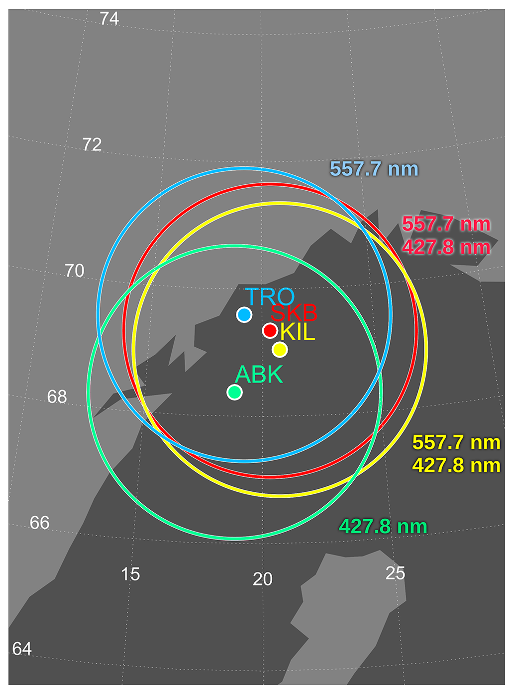
Figure 1 The fields of view of all-sky cameras in Abisko (ABK), Kilpisjärvi (KIL), Skibotn (SKB), and Tromsø (TRO) at an altitude of 100 km. The map is over northern Fennoscandia.

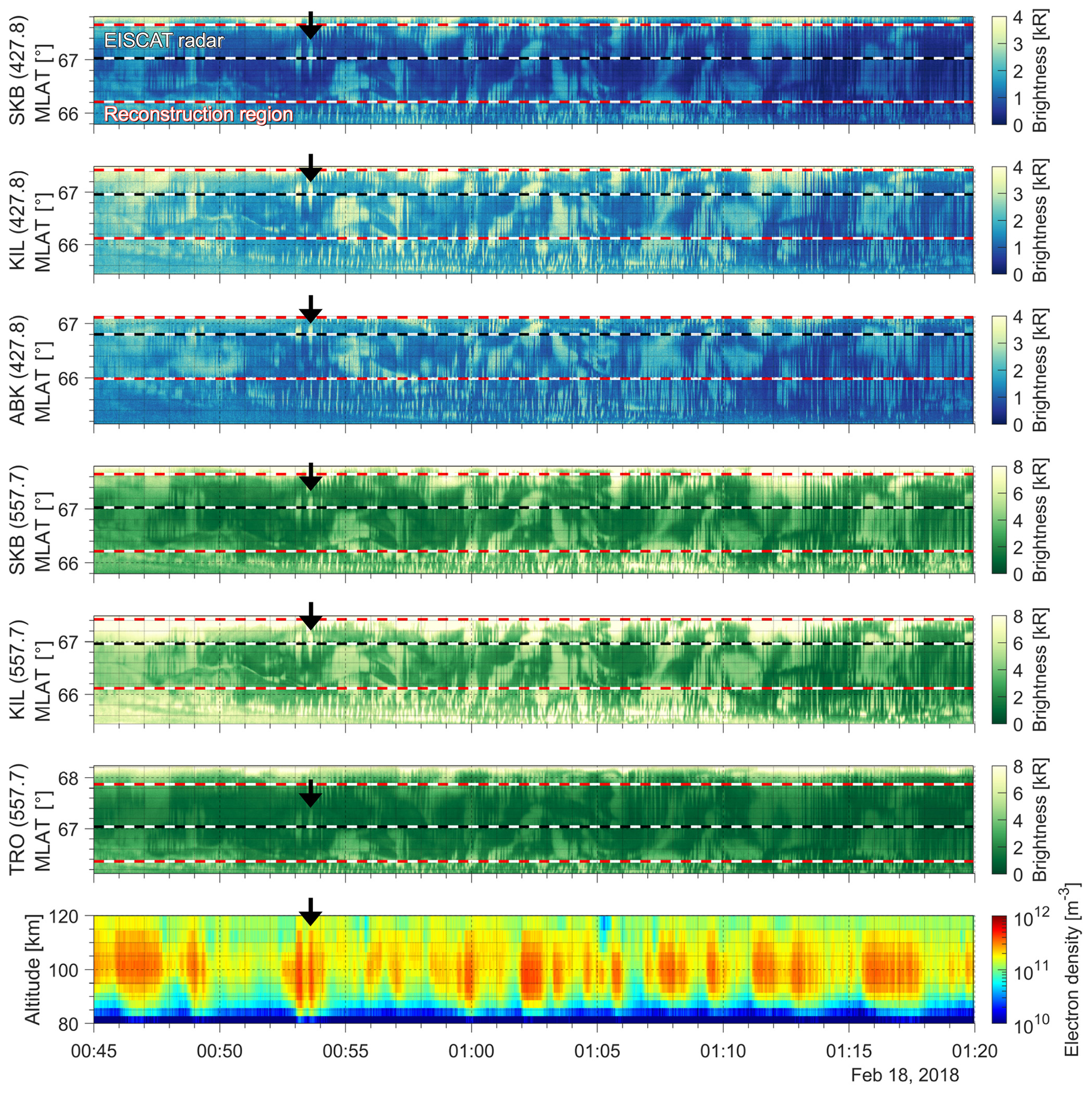
Figure 2 Keogram (time series of an auroral image sliced along the magnetic longitude or north–south-aligned direction to pass through the pixel containing the EISCAT radar observation point at 100 km altitude) at each station and each wavelength from 00:45 to 01:20 UT on 18 February 2018. The vertical axis is the magnetic latitude (MLAT). Black and red dashed lines show the EISCAT radar observation point and reconstruction region, respectively. The bottom panel shows electron density observed by the EISCAT radar in Tromsø. Black arrows indicate the pulsating auroral patch analyzed in this study.

The reconstructed volume emission rate was converted to the electron density using the continuity equation of the electron density (Eq. 4 in Fukizawa et al., 2022), i.e.,

$$\begin{array}{}\text{(10)}& {\displaystyle \frac{\partial n_{\mathrm{e}}}{\partial t}}=kL-{\mathit{\alpha }}_{\mathrm{eff}}{n}_{\mathrm{e}}^{\mathrm{2}},\end{array}$$

where n_e (m⁻³) is the electron density, L (m⁻³ s⁻¹) is the volume emission rate, k is a positive constant for converting the volume emission rate to the ionization rate (see Appendix B in Fukizawa et al., 2022), and α_eff (m³ s⁻¹) is the effective recombination rate. Equation (10) was solved with the Runge–Kutta method. Using three effective recombination coefficients, Fukizawa et al. (2022) confirmed that the electron density observed by the EISCAT radar is within the calculated electron densities.

2.3 Optical observations

We used monochromatic auroral images obtained with ASCs at four ground-based stations: Abisko (ABK: 68.36^∘ N, 18.82^∘ E), Kilpisjärvi (KIL: 69.05^∘ N, 20.78^∘ E), Skibotn (SKB: 69.35^∘ N, 20.36^∘ E), and Tromsø (TRO: 69.58^∘ N, 19.22^∘ E). ASCs to observe 427.8 nm auroral emission were installed at ABK, KIL, and SKB, while those for 557.7 nm were at KIL, SKB, and TRO. The field of view of each ASC at an altitude of 100 km is shown in Fig. 1. ASCs for 427.8 nm at ABK and KIL were from the aurora observation network called the Magnetometers Ionospheric Radars All-sky Cameras Large Experiment (MIRACLE) (Sangalli et al., 2011). The filter wavelength attached to the MIRACLE ASCs is 427.8 ± 2 nm. The other ASCs were Watec Monochromatic Imagers (WMIs) (Ogawa et al., 2020a). The filter wavelengths of WMIs were 430 ± 5 and 560 ± 5 nm. The pixel numbers were 512 × 512 pixels for MIRACLE ASCs and 640 × 480 pixels for WMIs. The exposure time was 1 s to observe the 557.7 nm emission but 2 s for the dimmer 427.8 nm emission. The 557.7 nm auroral images were integrated every 2 s to match the time resolution of the 427.8 nm auroral images. To improve the signal-to-noise ratio, we composited 427.8 nm auroral images obtained from four same-type WMIs at SKB. In addition, the median filter of 3 × 3 pixels was applied to all the auroral images. When the same median filter was applied to dark images subtracted from the auroral images, unexpected small structures appeared in the subtracted auroral images. To avoid this over-subtraction, we applied a 7 × 7 pixel median filter for the dark images. After the subtraction of the dark images, we conducted the flat-field correction, Gamma correction, and conversion from count to Rayleigh. The relationship between count and Rayleigh can be written as the following equations.

$$\begin{array}{}\text{(11)}& {\displaystyle }\left[{\mathrm{Count}}^{\prime }\right]=\mathrm{255}\times {\left(\left[\mathrm{Count}\right]/\mathrm{255}\right)}^{\left(\mathrm{1}/\mathit{\gamma }\right)}\text{(12)}& {\displaystyle }\left[\mathrm{Rayleighs}\right]=a\times \left[{\mathrm{Count}}^{\prime }\right]+b\end{array}$$

Here, Count is the raw count, Count^′ is the Gamma-corrected count, γ is the Gamma value, and a and b are constants. The constants a and b were determined by the National Institute of Standards and Technology (NIST) traceable 1.9 m integration sphere (Labsphere LMS-760) at the National Institute of Polar Research (NIPR) (Ogawa et al., 2020b). The parameters are summarized in Table 1.

Table 1 Filter wavelength and constants in Eqs. (11), (12), and (13) for each camera. c and d values are only for the 00:53:36 UT time point shown in Fig. 4.

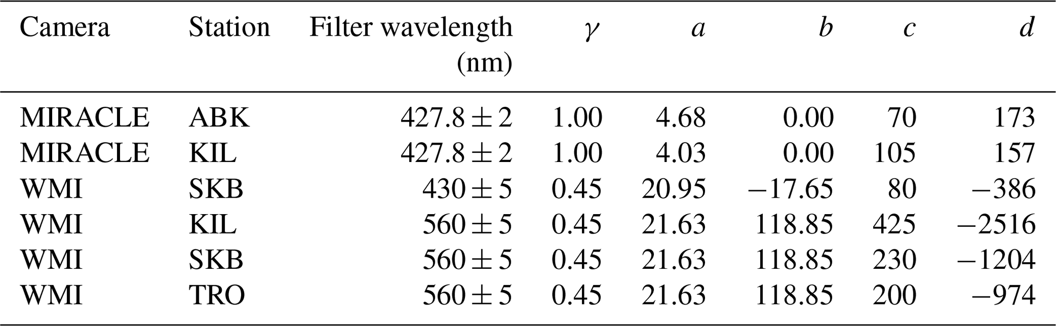
Figure 2a–f show, at each station and each wavelength, the keogram, which is the time series of the auroral image sliced along the magnetic longitude to pass through the pixel containing the EISCAT radar observation point from 00:45 to 01:20 UT on 18 February 2018. After an auroral breakup at 00:10 UT, diffuse auroras, PsAs, and auroral streamers were observed by ASCs at the stations except for KIL (Video A1, Fukizawa, 2023). It was cloudy at KIL until 00:47 UT. A PsA patch was detected at the EISCAT radar observation pixel at 00:53:30–00:53:42 UT, as shown by the black arrows in Fig. 2. The electron density increased in association with the PsA patch even below 85 km altitude (Fig. 2). As shown in Fig. 3, this PsA patch was classified as an expanding PsA, which expands from a core and then recedes back.

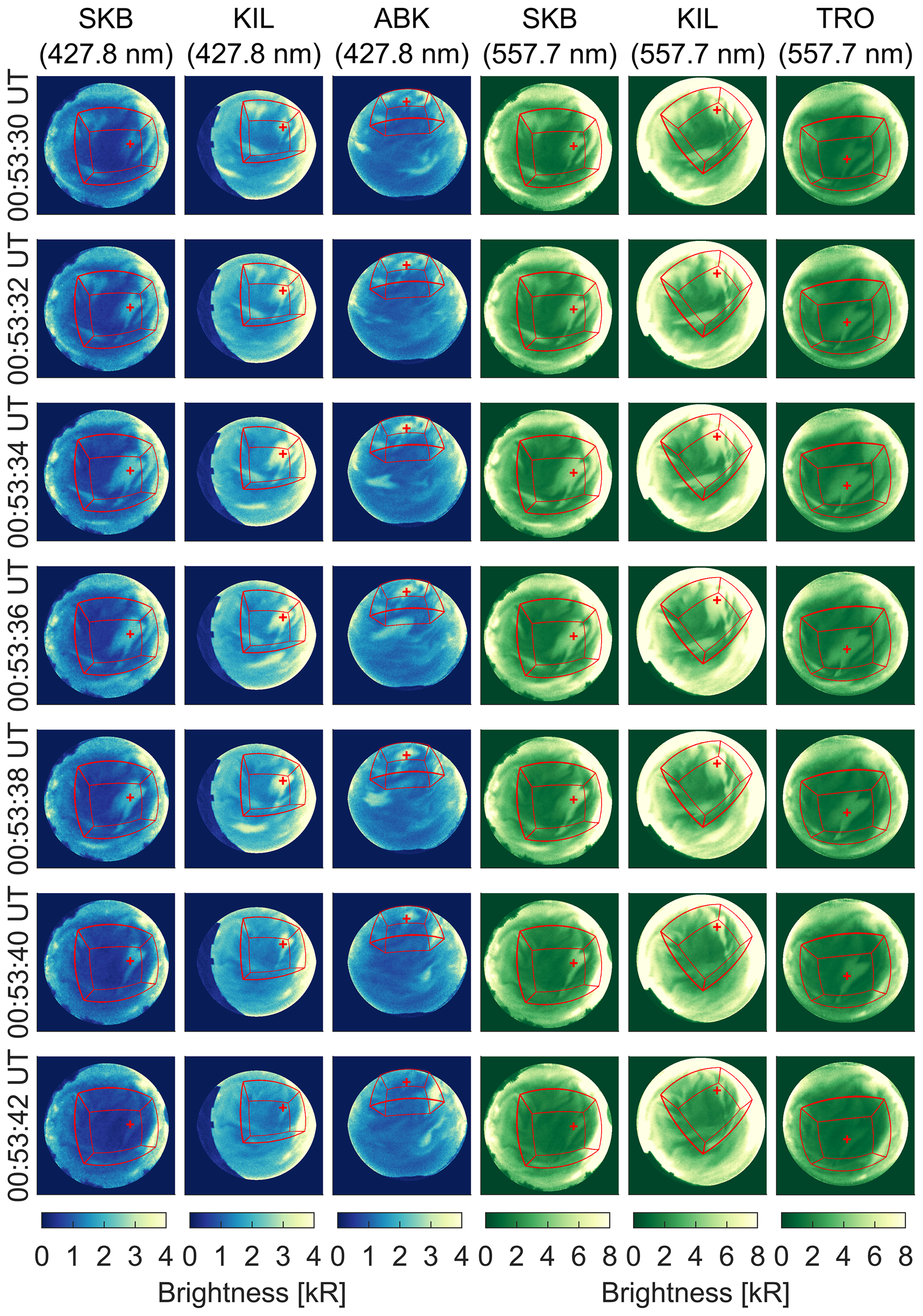
Figure 3 The 427.8 and 557.7 nm auroral images obtained from all-sky cameras in ABK, KIL, SKB, and TRO from 00:53:30 to 00:53:42 UT on 18 February 2018. The red plus and lines represent the EISCAT radar observation pixel and reconstruction region boundaries, respectively.

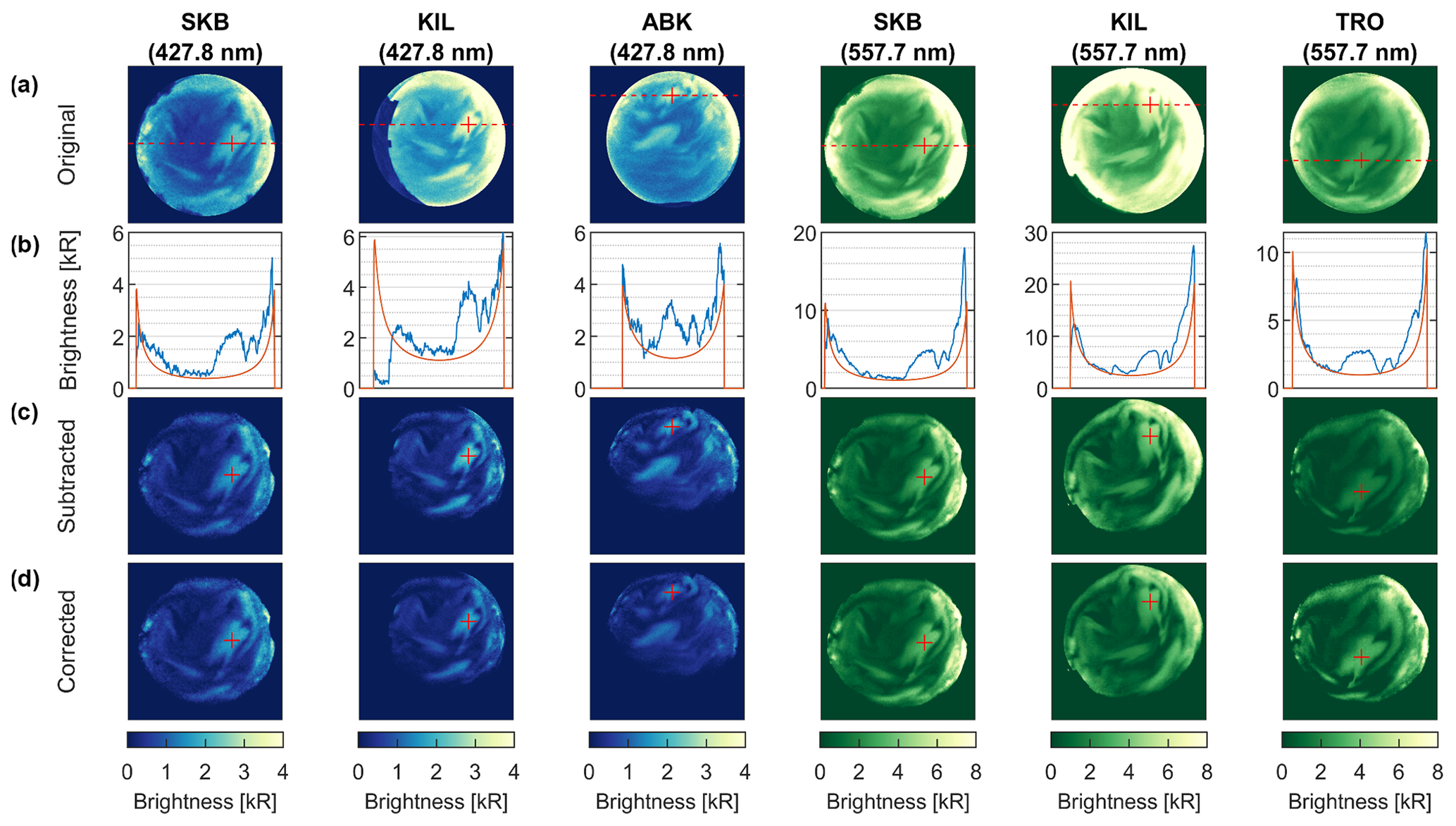
Figure 4 (a) Observed auroral images at 00:53:36 UT on 18 February 2018. Red pluses represent EISCAT radar observation pixels. (b) Brightness of observed auroral images (blue lines) and estimated background emission (orange lines) along the red dashed lines in panel (a). (c, d) Auroral images with (c) background emission subtracted and (d) relative sensitivity corrected.

The PsA emissions in the auroral images were embedded in emissions such as diffuse aurora, sunlight, moonlight, and city light (Fig. 4a–b). These background emissions, which have no specific structure, should be subtracted before conducting G-ACT because they cause ambiguity in the reconstruction results. The background emission image g_bk was defined as

$$\begin{array}{}\text{(13)}& {\mathit{g}}_{\mathrm{bk}}=c{\mathit{g}}_{\mathrm{0}}+d,\end{array}$$

where g₀ (R) is a modeled image derived by assuming all the voxels had the same volume emission rate of 1 cm⁻³ s⁻¹, $d=min\left(\stackrel{\mathrm{̃}}{\mathit{g}}\right)-min\left(c{\mathit{g}}_{\mathrm{0}}\right)$, and c is a constant whose value is chosen to minimize $|\stackrel{\mathrm{̃}}{\mathit{g}}-{\mathit{g}}_{\mathrm{bk}}{|}^{\mathrm{2}}$. We did not use pixel values with a zenith angle larger than 80^∘. The determined background emission profiles are shown with orange lines in Fig. 4b. The values of c and d in Eq. (13) differ because the zenith angle of the sun or moon and the brightness of city light depend on the position of the observation point (Table 1). These values also varied with time due to temporal variation in diffuse auroral emission intensity. Figure 4c shows auroral images with background emission subtracted. The background removal could cause the underestimation of reconstructed volume emission rates if the background emission is dominated by diffuse auroral emission in the E region. This possibility is discussed in Sect. 4. Pixel values below 0 were set to 1 before tomographic analysis was performed.

Although the absolute value of the auroral image from each ASC has been corrected by calibration experiments in a laboratory, the images from different ASCs had different absolute values during actual observations due to differences in the sensitivity degradation and transmission of acrylic domes at each station. These differences were corrected by the parameter c_j in Eq. (7). The method to determine this parameter is explained in the next section.

2.4 Determination of hyperparameters

Before conducting G-ACT, the hyperparameters λ and c_j in Eq. (7) must be determined. First, we determined c_j (j=1, 2, …, 6) with λ fixed at 10⁻⁵ using fivefold cross-validation (Stone, 1974). Elements of the observed auroral image vector $\stackrel{\mathrm{̃}}{\mathit{g}}$ were divided into five subsets. Then, one subset was selected as the test set (${\stackrel{\mathrm{̃}}{\mathit{g}}}_j^{\mathrm{tes}}$) and the others as the training set (${\stackrel{\mathrm{̃}}{\mathit{g}}}_j^{\mathrm{tra}}$). We found the solution $\widehat{x}$ to minimize $\mathit{\phi }(\mathit{x};\mathit{\lambda },c_j)$ using only the training set ${\stackrel{\mathrm{̃}}{\mathit{g}}}_j^{\mathrm{tra}}$ and then predicted the test set ${\mathit{g}}_j^{\mathrm{tes}}\left(\widehat{x}\right)$. We then calculated the residual sum of squares between the actual and predicted values for the test data:

$$\begin{array}{}\text{(14)}& \mathit{\delta }\left(c_j\right)=\sum _j{∥c_j{\stackrel{\mathrm{̃}}{\mathit{g}}}_j^{\mathrm{tes}}-{\mathit{g}}_j^{\mathrm{tes}}\left(\widehat{x}\right)∥}^{\mathrm{2}}.\end{array}$$

The cross-validation score $\stackrel{\mathrm{‾}}{\mathit{\delta }}\left(c_j\right)$ was calculated by averaging over five values of δ(c_j), which were obtained by using a different set as the training set each time. To save computational cost, cross-validation was performed separately for each wavelength. The relative sensitivities of SKB were fixed to 1 for each wavelength, while the other relative sensitivities were determined using the grid search method. The determined values were 0.78 for ABK (427.8 nm), 0.73 for KIL (427.8 nm), 0.61 for KIL (557.7 nm), and 1.92 for TRO (557.7 nm). Auroral images with relative sensitivity corrected are shown in Fig. 4d.

The value of the parameter λ was selected so as to minimize the difference between the electron densities observed by the EISCAT radar and those reconstructed by G-ACT. We conducted G-ACT for $\mathit{\lambda }={\mathrm{10}}^{-\mathrm{5}}$, 10⁻⁴, 10⁻³, 10⁻², 10⁻¹, and 10⁰ and found that the difference reached a minimum at $\mathit{\lambda }={\mathrm{10}}^{-\mathrm{1}}$.

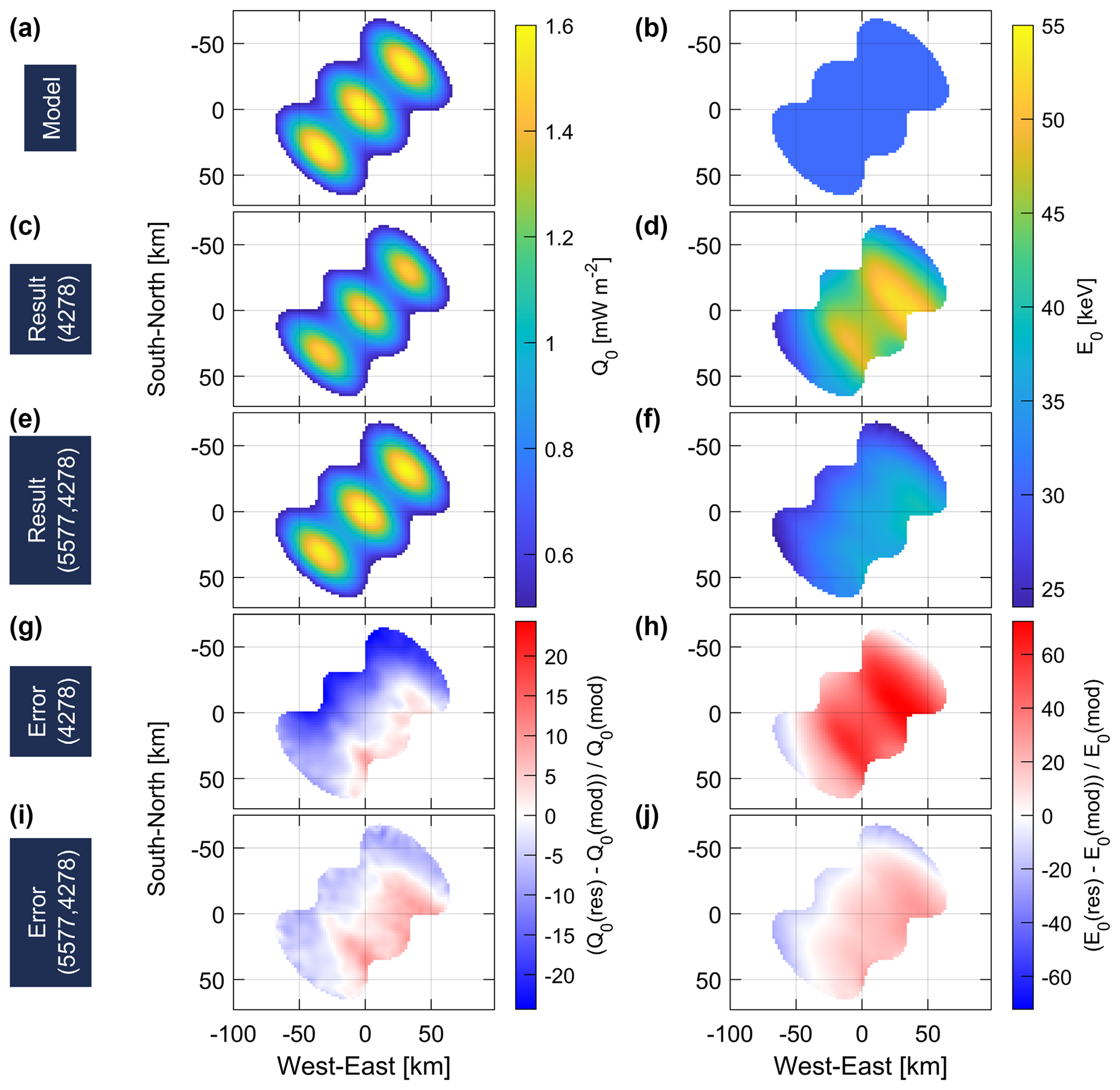
Figure 5 Models of (a) the total energy flux Q₀ and (b) average energy E₀. (c–f) Reconstructed results of (c, e) the total energy flux and (d, f) average energy using (c, d) only 427.8 nm auroral images or (e, f) both 557.7 and 427.8 nm auroral images. (g–j) Relative reconstruction errors are calculated as (result − model) $/$ model.

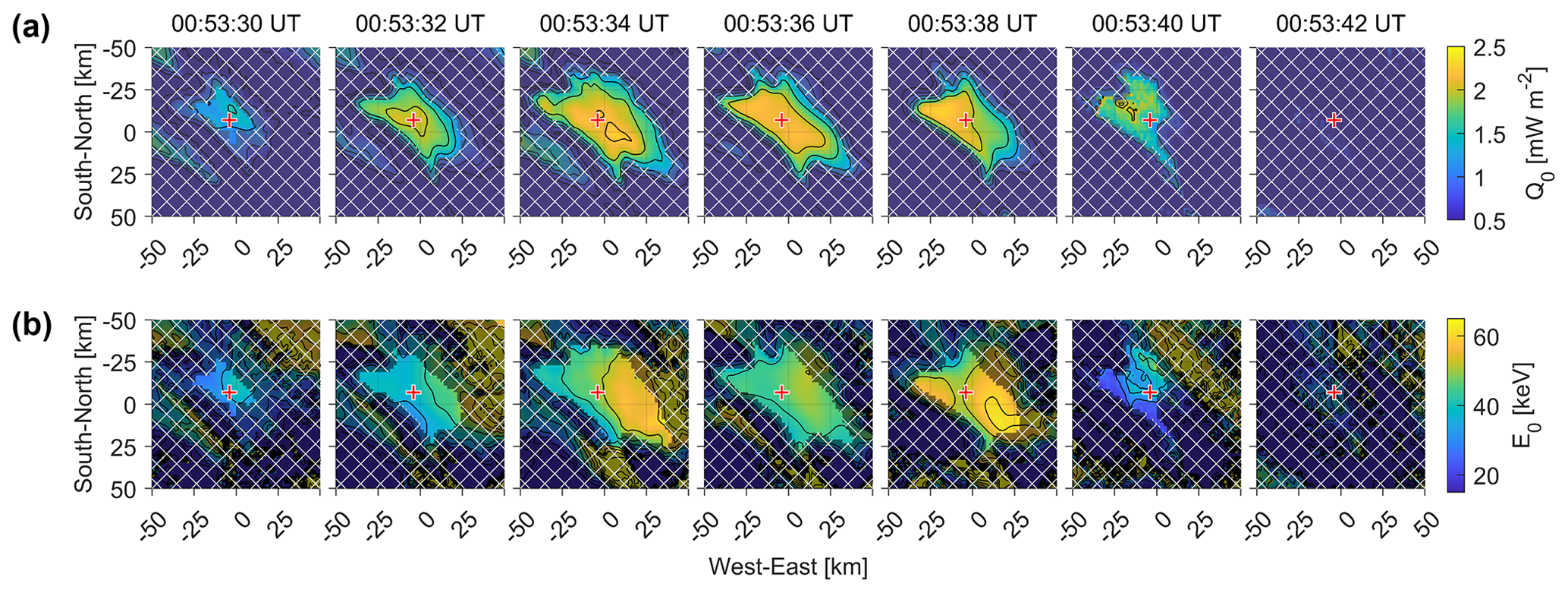
Figure 6 (a) The total energy flux Q₀ and (b) average energy E₀ of the reconstructed electron flux. The pixels where the total energy flux was less than 1.0 mW m⁻² are hatched by white lines. Red pluses represent the EISCAT radar observation point.

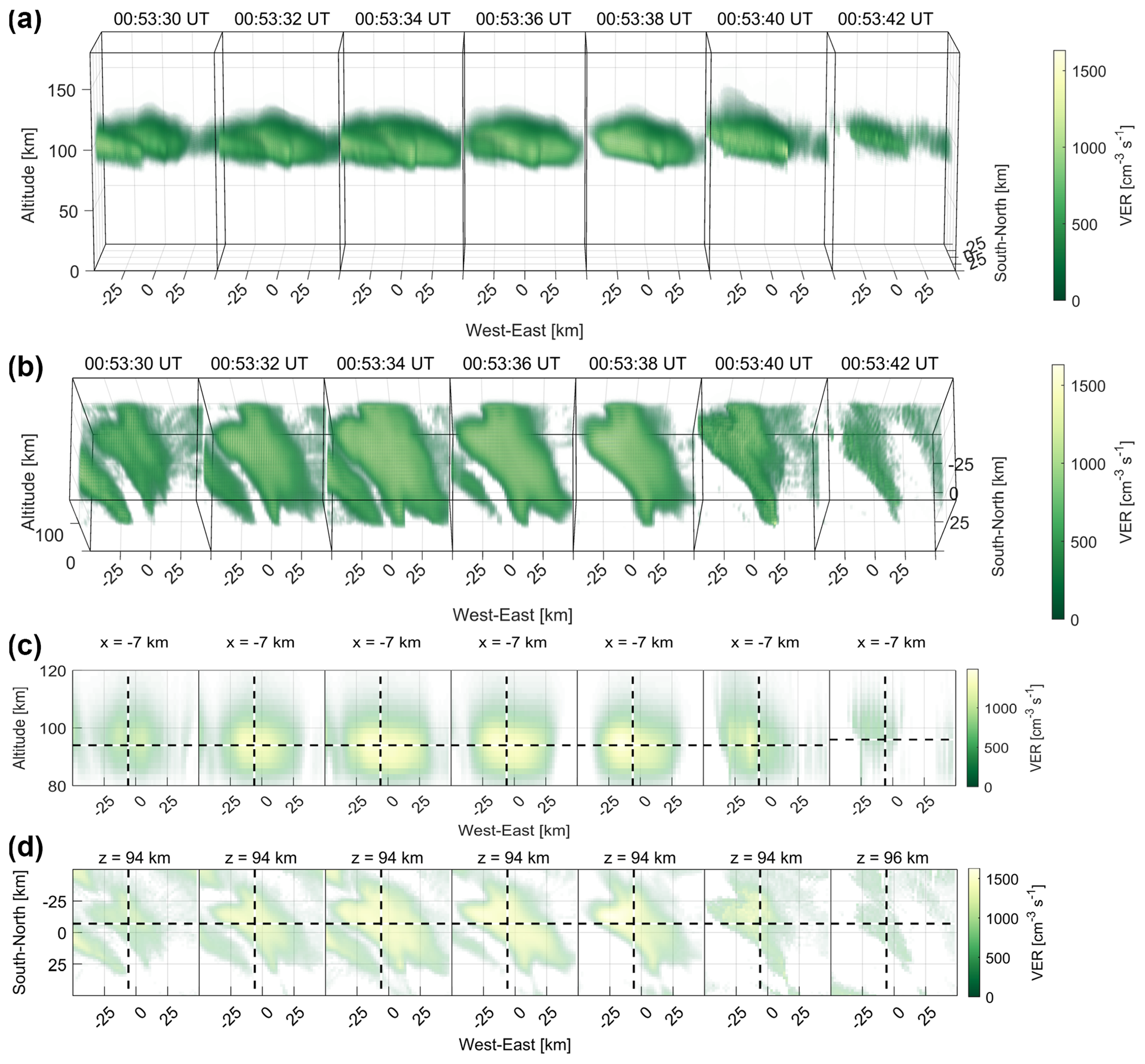
Figure 7 (a, b) The 3-D distribution of the reconstructed volume emission rate (VER) at a wavelength of 557.7 nm viewed from different elevation angles. (c) Cross sections parallel to the magnetic field lines and (d) horizontal cross sections containing peak values on the EISCAT radar beam. Vertical and horizontal dashed lines show the EISCAT radar beam and the altitude of the peak volume emission rate, respectively. The transparency depends on the VER values. The minimum VER is invisible, and the maximum VER is opaque.

2.5 Validation of reconstruction accuracy using model aurora

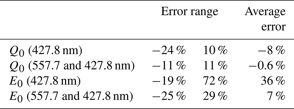
In Fukizawa et al. (2022), PsA patches were reconstructed using only 427.8 nm auroral images at three stations (ABK, KIL, and TRO). By contrast, we improved the G-ACT method by adding auroral images at another wavelength (557.7 nm) at three stations (KIL, SKB, and TRO). The total number of stations was increased from three to four due to the addition of TRO. We performed G-ACT for a model aurora to determine the extent of reconstruction accuracy improvement associated with including the additional wavelength and observation point. First, horizontal distributions of total energy flux and average energy were prepared for three adjacent patches. The total energy flux was assumed to have a Gaussian distribution with a peak value of 1.6 mW m⁻² (Fig. 5a). A uniform distribution with a value of 30 keV was assumed for the average energy (Fig. 5b). Second, the 3-D distributions of the volume emission rate at wavelengths of 427.8 and 557.7 nm were derived using the GLOW model. Third, modeled auroral images were obtained by integrating the 3-D volume emission rates from the various observation points. Random noises from a normal distribution with a mean value of 0 and a standard deviation determined from observed auroral images were added to the modeled images. Fourth, the total energy flux and average energy were reconstructed using only 427.8 nm images (Fig. 5c–d) and using both 557.7 and 427.8 nm images (Fig. 5e–f). Finally, relative errors between the reconstructed and modeled total energy fluxes and between the reconstructed and modeled average energies were calculated as error = (result − model) $/$ model (Fig. 5g–j). The total energy flux and average energy were underestimated in the northwest and overestimated in the southeast, but the use of auroral images at both 557.7 and 427.8 nm showed a decrease in error compared to the use of only the 427.8 nm images. Error ranges and average errors for the total energy flux and average energy are listed in Table 2.

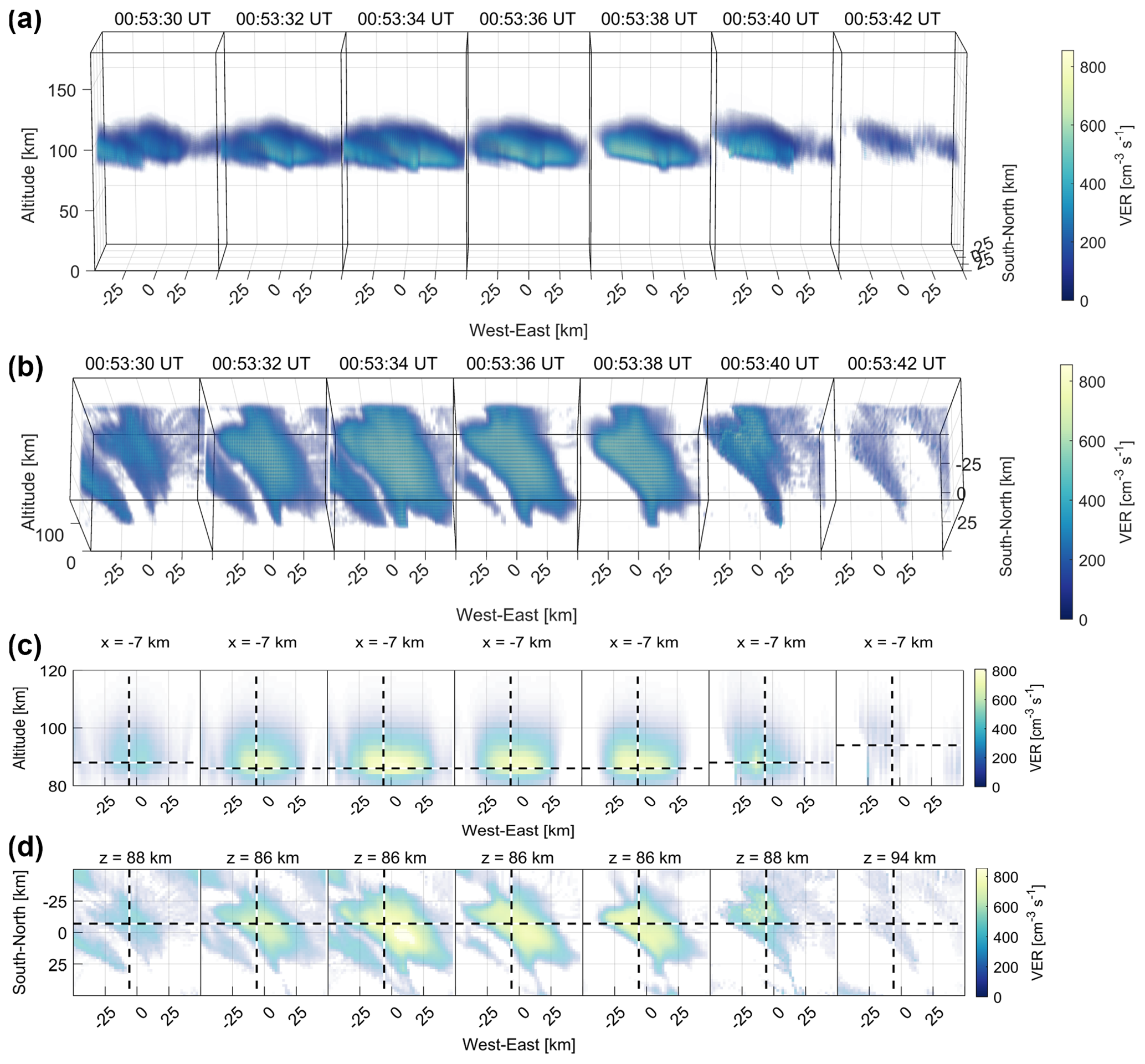
Figure 8 The reconstructed volume emission rate at a wavelength of 427.8 nm. The figure format is the same as that of Fig. 7.

Table 2 Errors of the total energy flux (Q₀) and average energy (E₀) reconstructed using only 427.8 nm auroral images vs. using both 557.7 and 427.8 nm auroral images. Error ranges and average errors are listed. The errors were calculated as (result − model) $/$ model.

3 Results

3.1 G-ACT reconstruction results

The precipitating electron fluxes and volume emission rates at wavelengths of 557.7 and 427.8 nm were reconstructed from auroral images using G-ACT. Figure 6 depicts the total energy flux and average energy of the reconstructed precipitating electron flux. The total energy flux reached its maximum value of ∼ 2.5 mW m⁻² near the central part of the PsA patch from 00:53:34 to 00:53:38 UT. The average energy reached its maximum value of ∼ 62 keV at 00:53:38 UT.

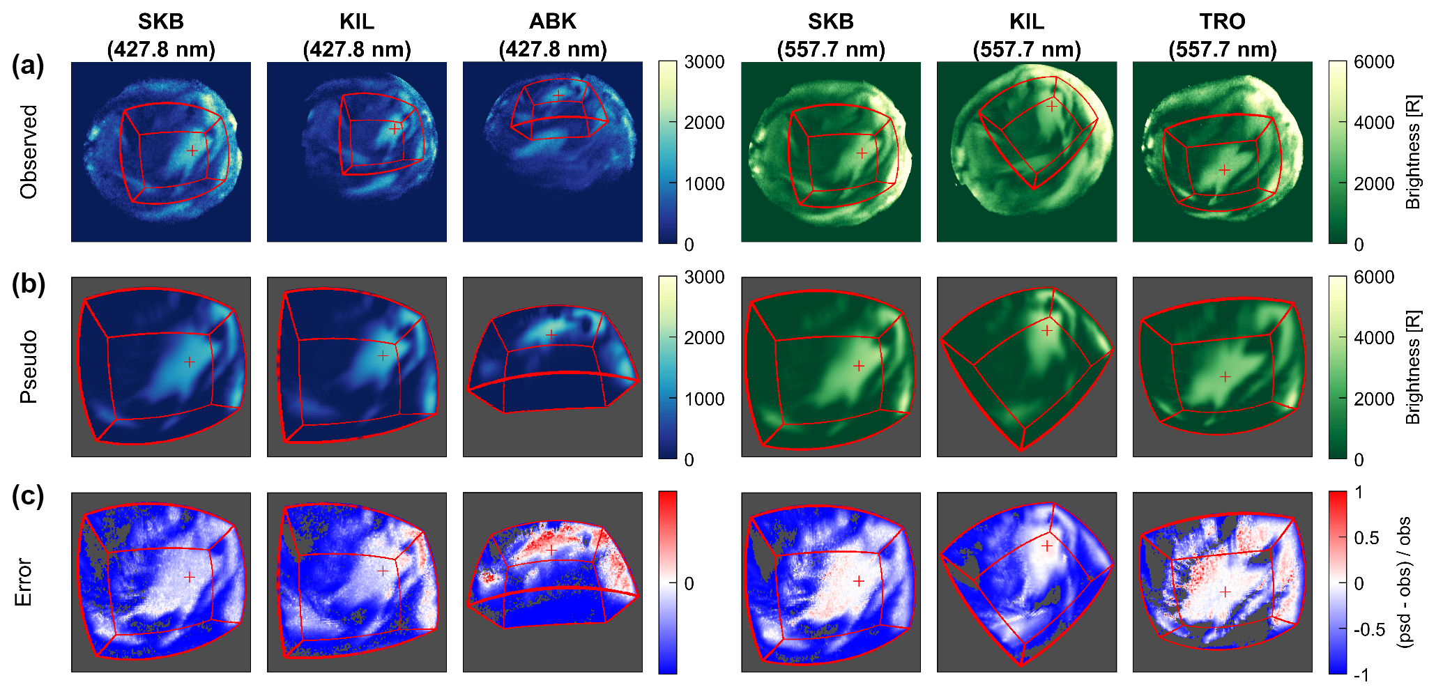
Figure 9 (a) Observed auroral images at 00:53:36 UT on 18 February 2018. Red pluses and lines represent the EISCAT radar observation pixel and the reconstruction region boundaries, respectively. (b) Modeled auroral images calculated from the reconstructed volume emission rate. (c) Relative errors calculated as [(b) − (a)] $/$ (a). Errors with an observed auroral brightness of less than 100 are not shown.

Figures 7 and 8 illustrate the 3-D distribution of the reconstructed volume emission rate at wavelengths of 557.7 and 427.8 nm, respectively. The peak altitudes of the volume emission rate along the EISCAT radar beam were approximately 94 km for 557.7 nm and 86 km for 427.8 nm (Figs. 7c, d and 8c, d). To validate the G-ACT reconstruction results, the difference between the observed auroral image (Fig. 9a) and the modeled auroral image (Fig. 9b) obtained by integrating the reconstructed volume emission rates from the various stations was calculated and is shown in Fig. 9c. The observed auroral images were almost perfectly reconstructed except for images at ABK, for which the reconstruction region lay near the edge of the ASC's field of view. One of the reasons for this error was that the ground stations were biased to the south of the analyzed PsA patch. Therefore, increasing the number of observation points from the north or targeting an auroral structure closer to the centroid of the observation points is expected to mitigate this error.

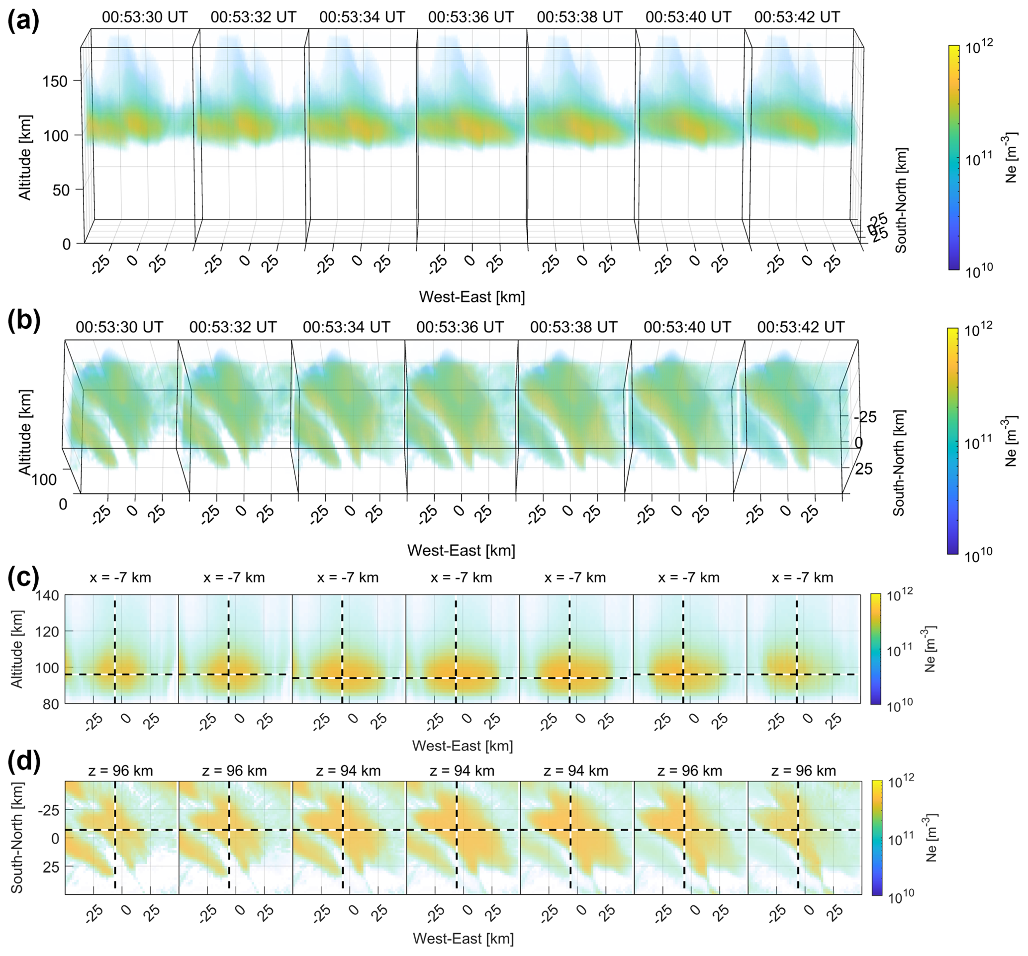
Figure 10 (a, b) Reconstructed 3-D electron density (N_e) viewed from different elevation angles. (c) Cross sections parallel to the magnetic field lines and (d) horizontal cross sections containing peak values on the EISCAT radar beam. Vertical and horizontal dashed lines represent the EISCAT radar beam and the altitude of the peak electron density, respectively.

3.2 Three-dimensional Pedersen and Hall conductivities

As explained in Sect. 2.2, the electron density was derived from the reconstructed volume emission rate at 427.8 nm (Fig. 8) using the Runge–Kutta method to solve the continuity equation of the electron density (Eq. 10). Figure 10 depicts the reconstructed 3-D electron density. The effective recombination coefficient used was (Gledhill, 1986)

$$\begin{array}{}\text{(15)}& \begin{array}{rl}{\mathit{\alpha }}_{\mathrm{fit}}=& \mathrm{4.30}\times {\mathrm{10}}^{-\mathrm{12}}\exp \left(-\mathrm{2.42}\times {\mathrm{10}}^{-\mathrm{2}}z\right)\\ & +\mathrm{8.16}\times {\mathrm{10}}^{\mathrm{6}}\exp \left(-\mathrm{0.524}z\right)\left({\mathrm{m}}^{\mathrm{3}}{\mathrm{s}}^{-\mathrm{1}}\right),\end{array}\end{array}$$

where z (km) is the altitude. Gledhil (1986) derived Eq. (15) using the least-squares method for 122 data points of the effective recombination coefficient obtained from 18 previous studies (references in Gledhil, 1986). The peak electron density on the EISCAT radar beam occurred at an altitude of almost 94–96 km (Fig. 10c and d). The method of solving the continuity equation of the electron density accounted for time variation and thus was able to show that the electron density remained high even after the brightness of the aurora faded at 00:53:42 UT. To evaluate the reconstruction accuracy of the electron density, the reconstructed altitudinal profile of electron density was compared with that observed by the EISCAT radar (Fig. 11a). In addition to the effective recombination coefficient of Eq. (15), two coefficients were used as the upper and lower bounds on α_eff in Eq. (10) (Semeter and Kamalabadi, 2005), i.e.,

$$\begin{array}{}\text{(16)}& {\displaystyle }{\mathit{\alpha }}_{{\mathrm{NO}}^{+}}=\mathrm{4.2}\times {\mathrm{10}}^{-\mathrm{13}}{\left(\mathrm{300}/T_{\mathrm{n}}\right)}^{\mathrm{0.85}}\left({\mathrm{m}}^{\mathrm{3}}{\mathrm{s}}^{-\mathrm{1}}\right),\text{(17)}& {\displaystyle }{\mathit{\alpha }}_{{\mathrm{O}}_{\mathrm{2}}^{+}}=\mathrm{1.95}\times {\mathrm{10}}^{-\mathrm{13}}{\left(\mathrm{300}/T_{\mathrm{n}}\right)}^{\mathrm{0.7}}\left({\mathrm{m}}^{\mathrm{3}}{\mathrm{s}}^{-\mathrm{1}}\right),\end{array}$$

where T_n (K) is the neutral temperature. The observed electron densities lay mostly within the electron density distribution obtained using the three effective recombination coefficients. Especially below about 90 km altitude, the electron density calculated using Eq. (15) was the most consistent with the observed electron density. Therefore, we used Eq. (15) to calculate the electron density in Fig. 10. The Pedersen and Hall conductivities were calculated by substituting the reconstructed electron density (Fig. 10) into Eqs. (1) and (2). Figures 12 and 13 illustrate the 3-D distribution of the reconstructed Hall and Pedersen conductivities. The Hall conductivity reached its maximum value of 1.4 × 10⁻³ S m⁻¹ at 94 km altitude, while the Pedersen conductivity reached its maximum value of 2.6 × 10⁻⁴ S m⁻¹ at 116 km altitude. The Pedersen conductivity showed a secondary peak of 9.9 × 10⁻⁵ S m⁻¹ at 86 km altitude. The electron Pedersen conductivity maximum value in the D region was approximately 38 % of the ion Pedersen conductivity maximum value in the E region compared to a figure of 13 % in Hosokawa and Ogawa (2010). The altitude profiles of the reconstructed Hall and Pedersen conductivities were compared with those calculated from the electron densities observed by the EISCAT radar (Fig. 11b and c). Although the Pedersen conductivity values reconstructed by G-ACT were overestimated in the D region compared to those of the EISCAT radar by a factor of 1.2–1.5, the D-region Pedersen conductivity peak values derived from the EISCAT radar were also 25 %–44 % of those in the E region, in keeping with the G-ACT results.

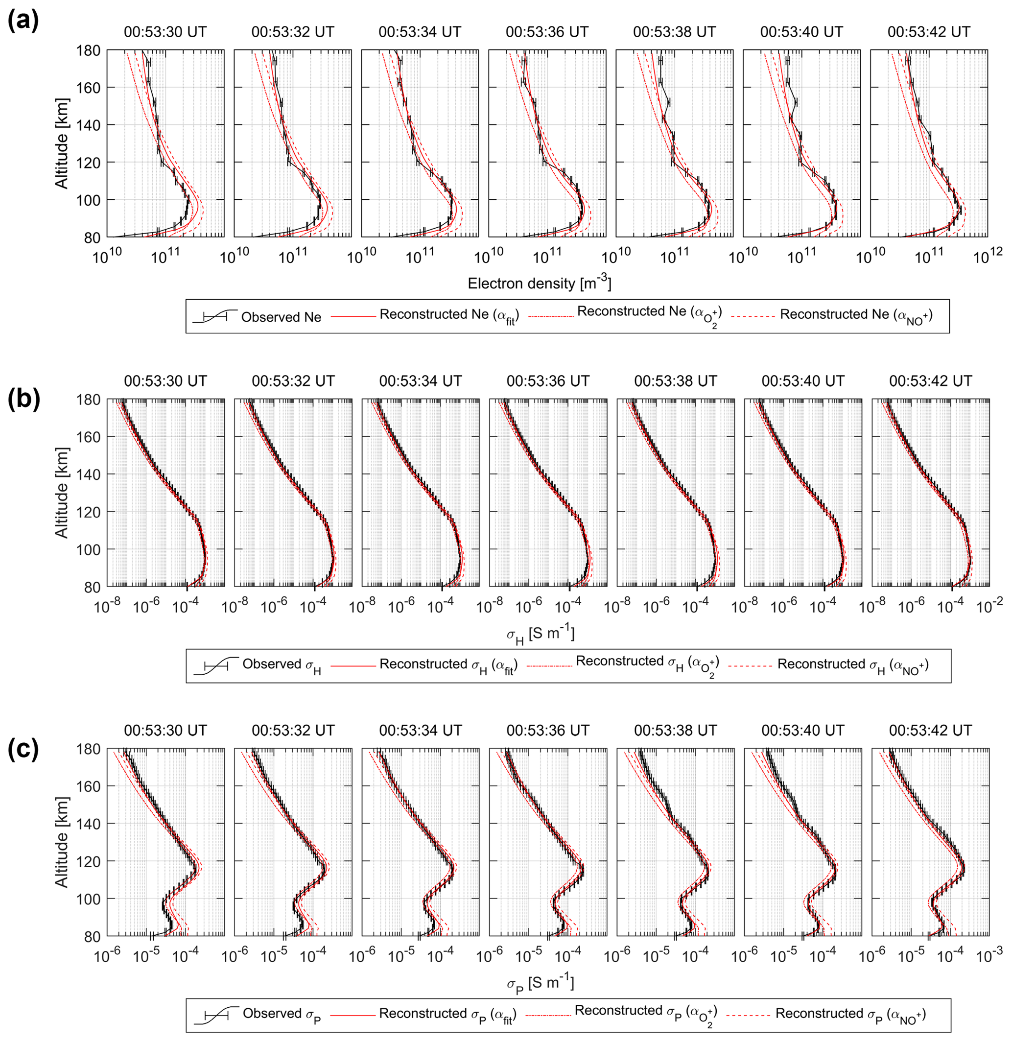
Figure 11 Altitude profiles of the reconstructed (red lines) and observed (black lines) (a) electron density, (b) Hall conductivity, and (c) Pedersen conductivity. Error bars represent measurement uncertainties.

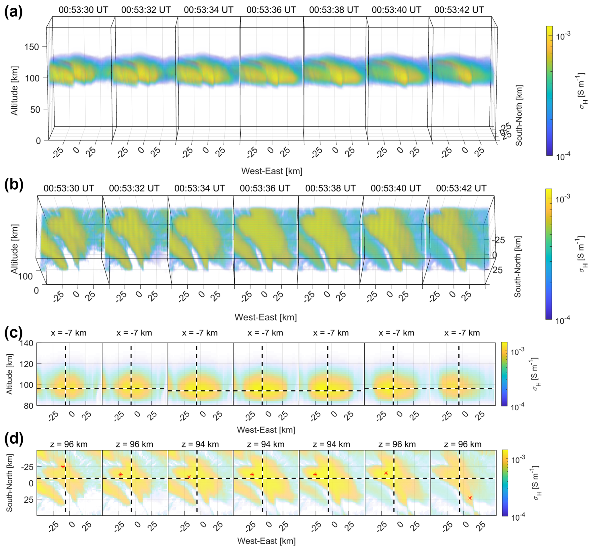
Figure 12 (a, b) The 3-D distribution of the reconstructed Hall conductivity. (c) Cross sections parallel to the magnetic field lines and (d) a horizontal cross section containing peak values on the EISCAT radar beam. Vertical and horizontal dashed lines show the EISCAT radar beam and the altitude of the peak Hall conductivity, respectively. Red asterisks represent peak value positions within the center of the PsA patch.

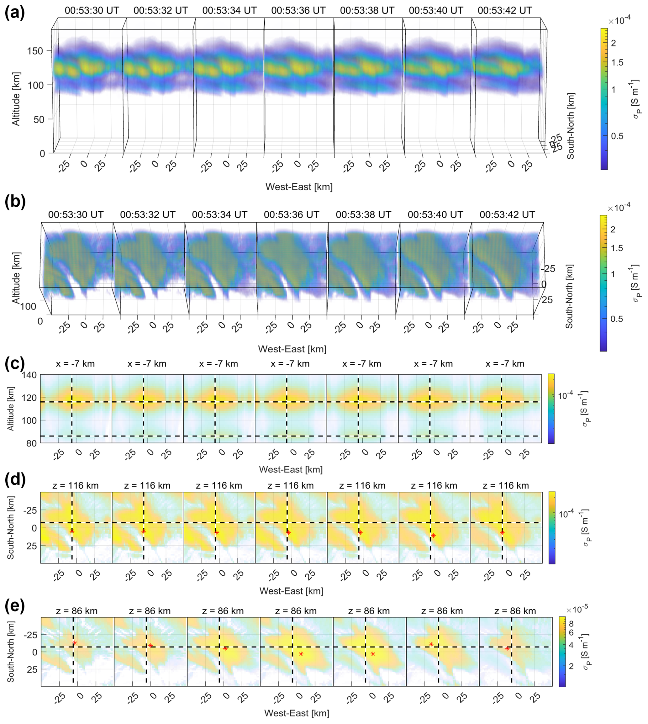
Figure 13 The 3-D distribution of the reconstructed Pedersen conductivity. The figure format is the same as that of Fig. 12.

4 Discussion

The horizontal distribution of the Pedersen conductivity in the D region varied significantly in space and time compared to the E region (Fig. 13d and e). The peak location in the horizontal planes differed between the electron and ion Pedersen layers. These altitudinal differences in the horizontal distribution of the Pedersen conductivity affect the closure of FACs associated with PsAs. It is expected that, in the future, the ionospheric conductivity obtained using the method proposed in this study will be combined with EISCAT_3D data to elucidate how the FACs associated with PsAs are closed in the ionosphere.

Three-dimensional electric field data, which will be obtained in the future by EISCAT_3D radar observations, are not available at present. However, the electric field is often assumed to be uniform around PsAs, since PsA patches often drift uniformly with the E×B drift velocity (Hosokawa et al., 2010; Hosokawa and Ogawa, 2010; Oguti et al., 1984; Yang et al., 2015). Therefore, we evaluated the amount of FAC caused solely by the nonuniform distribution of ionospheric conductivity under the assumption of a uniform electric field. According to the current continuity, the FAC, j_∥ (A m⁻²), is equal to the divergence of the height-integrated current perpendicular to the magnetic field lines, J_⊥ (A m⁻¹). Using the current continuity and the ionospheric Ohm law, the FAC can be written as

$$\begin{array}{}\text{(18)}& \begin{array}{rl}{\mathit{j}}_{\parallel }=& {\mathrm{\nabla }}_{\perp }\cdot {\mathbf{J}}_{\perp }\\ =& \left({\mathrm{\nabla }}_{\perp }{\mathbf{\Sigma }}_{\mathrm{P}}\right)\cdot {\mathbf{E}}_{\perp }+{\mathbf{\Sigma }}_{\mathrm{P}}\left({\mathrm{\nabla }}_{\perp }\cdot {\mathbf{E}}_{\perp }\right)\\ & -\left({\mathrm{\nabla }}_{\perp }{\mathbf{\Sigma }}_{\mathrm{H}}\right)\cdot \left({\mathbf{E}}_{\perp }\times \mathit{b}\right)-{\mathbf{\Sigma }}_{\mathrm{H}}\mathit{b}\cdot \left({\mathrm{\nabla }}_{\perp }\times {\mathbf{E}}_{\perp }\right),\end{array}\end{array}$$

where Σ_P and Σ_H (S) are the height-integrated Pedersen and Hall conductivities, respectively, E_⊥ (V m⁻¹) is the ionospheric electric field perpendicular to the magnetic field, and b is the unit vector of the geomagnetic field. We assumed a uniform southward E_⊥, allowing the second and fourth terms in Eq. (18) to be ignored. The E_⊥ amplitude was estimated to be 12.5 mV m⁻¹ from the ionospheric convection velocity obtained from Super Dual Auroral Radar Network (SuperDARN) (Greenwald et al., 1995) observations (∼ 250 m s⁻¹) and assuming B ≈ 50 000 nT. Consequently, the maximum downward and upward FACs were 69 and 68 µA m⁻² at the northeastern and southwestern edges of the PsA patch, respectively. These FACs are approximately 10 times larger than those observed by magnetometers on board satellites (Gillies et al., 2015). It is possible that the PsA patches analyzed in this study actually had such large FACs, given that their boundaries were sharper than those of Gillies et al. (2015). Gillies et al. (2015) may also have underestimated the FAC by ∼ 50 µA m⁻² around 67^∘ magnetic latitude, where the PsA patch was detected in this study, according to Fig. 4 in Ritter et al. (2013). If our results are overestimated, mainly there are two main factors. One is that the uniform E_⊥ assumption may not be reasonable. Indeed, higher conductivities drive the polarization of the electric field inside PsA patches (Hosokawa et al., 2010; Takahashi et al., 2019). The 3-D distribution of the ionospheric electric field will be obtained with the EISCAT_3D radar in the near future, settling this question. The other factor is the background emission subtraction from the auroral images before conducting G-ACT. Background emission subtraction enabled accurate reconstruction within the PsA patch. However, the conductivity outside the patch will be underestimated if the subtracted background emission contains mainly diffuse auroral emission. By contrast, if uniform diffuse auroral emission occurs around 150 km altitude, above PsAs, as reported by Brown et al. (1976), then the subtraction is not a problem because the horizontal gradient of electrical conductivity near the PsA patch is not affected by the subtraction. The peak altitude of auroral emissions or the characteristic energy of precipitating electrons can be estimated from the emission intensity ratio of 557.7–427.8 nm (Rees and Luckey, 1974; Steele and Mcewen, 1990). The intensity ratio of the removed background emission at 557.7 $/$ 427.8 was 2.8. This ratio indicates that the characteristic energies of the precipitating electrons was 1.6–4.0 keV (Fig. 4 in Rees and Luckey, 1974), ∼ 1.5–5 keV (Fig. 9 in Steele and Mcewen, 1990), or ∼ 20 keV using the GLOW model. Thus, the characteristic energy derived from the 557.7 $/$ 427.8 ratio depends on the models. The background emission intensity subtracted in our analysis was about 30 % of the observed pulsating auroral emission. Therefore, the volume emission rate of the background emission was calculated using the GLOW model and was multiplied by a constant so that the ratio of the linearly integrated volume emission rate in the altitude direction is 30 % of the volume emission rate of the reconstructed pulsating aurora. Then, the electron density was derived using the electron continuity equation by adding the calculated background emission to the reconstructed volume emission rate. We examined how much the electron density is underestimated at altitudes of 86, 96, and 116 km, where the Pedersen and Hall conductivities show peak values. For a characteristic energy of 1 keV, the electron density was underestimated by ∼ 30 %–40 % at an altitude of 116 km and remained the same at altitudes of 86 and 96 km. When the characteristic energy was 20 keV, the underestimation was ∼ 10 % at all three altitudes. The horizontal distribution of the ionospheric conductivity around PsA patches will be investigated by the EISCAT_3D radar in the near future.

5 Conclusions

In this study, G-ACT was used to reconstruct the 3-D distributions of the Hall and Pedersen conductivities of PsAs in order to elucidate the 3-D structures of ionospheric currents. The tomographic results show that the Hall conductivity peaked in the E region (altitudes of 94–96 km), while the Pedersen conductivity peaked in the E region (at 116 km altitude), with a secondary peak in the D region (at 86 km altitude). The electron Pedersen conductivity maximum value in the D region was approximately 38 % of the ion Pedersen conductivity maximum value in the E region; this ratio was nearly triple that reported by Hosokawa and Ogawa (2010). This result suggests that the Pedersen current in the D region caused by high-energy electron precipitation associated with PsAs has an outsized effect on FAC closure in the ionosphere.

Under the assumption of a uniformly distributed ionospheric electric field, derived FAC values near the edges of PsA patches were approximately 10 times higher than those reported by satellite observations. This overestimation means that the ionospheric electric field is not uniform and that the electrical conductivities around PsA patches may be underestimated. In the near future, the 3-D ionospheric conductivity reconstruction using G-ACT proposed in this study will be combined with 3-D observations of ionospheric conductivity and electric field strength by EISCAT_3D radar to elucidate the 3-D ionospheric current structures associated with PsAs.