Estimation and evaluation of hourly Meteorological Operational (MetOp) satellites' GPS receiver differential code biases (DCBs) with two different methods

Differential code bias (DCB) is one of the Global Positioning System (GPS) errors, which typically affects the calculation of total electron content (TEC) and ionospheric modeling. In the past, DCB was normally estimated as a constant in 1 d, while DCB of a low Earth orbit (LEO) satellite GPS receiver may have large variations within 1 d due to complex space environments and highly dynamic orbit conditions. In this study, daily and hourly DCBs of Meteorological Operational (MetOp) satellites' GPS receivers are calculated and evaluated using the spherical harmonic function (SHF) and the local spherical symmetry (LSS) assumption. The results demonstrated that both approaches could obtain accurate and consistent DCB values. The estimated daily DCB standard deviation (SD) is within 0.1 ns in accordance with the LSS assumption, and it is numerically less than the standard deviation of the reference value provided by the Constellation Observing System for Meteorology Ionosphere and Climate (COSMIC) Data Analysis and Archive Center (CDAAC). The average error's absolute value is within 0.2 ns with respect to the provided DCB reference value. As for the SHF method, the DCB's standard deviation is within 0.1 ns, which is also less than the standard deviation of the CDAAC reference value. The average error of the absolute value is within 0.2 ns. The estimated hourly DCB with LSS assumptions suggested that calculated results of MetOpA, MetOpB, and MetOpC are, respectively, 0.5 to 3.1 ns, −1.1 to 1.5 ns, and −1.3 to 0.7 ns. The root mean square error (RMSE) is less than 1.2 ns, and the SD is under 0.6 ns. According to the SHF method, the results of MetOpA, MetOpB, and MetOpC are 1 to 2.7 ns, −1 to 1 ns, and −1.3 to 0.6 ns, respectively. The RMSE is under 1.3 ns and the SD is less than 0.5 ns. The SD for solar active days is less than 0.43, 0.49, and 0.44 ns, respectively, with the LSS assumption, and the appropriate fluctuation ranges are 2.0, 2.2, and 2.2 ns. The variation ranges for the SHF method are 1.5, 1.2, and 1.2 ns, respectively, while the SD is under 0.28, 0.35, and 0.29 ns.

1 Introduction

The ionospheric variations affect radio communication and navigation, and ionosphere observations and modeling are still hot topics in space weather research.. Although there have been quite a lot of studies on the ionosphere, the topside ionosphere is quite difficult to model due to the lack of directly observed data (Jin et al., 2021). At present, many low Earth orbit (LEO) satellites carried Global Positioning System (GPS) receivers for accurate orbit determination, and topside ionospheric total electron content (TEC) can be obtained by using the dual-frequency GPS data. However, accurate TEC estimation from LEO satellite GPS observations is complicated due to the large number of effects or errors. The differential code bias (DCB) is one of the errors in calculating TEC due to complex space environments and highly dynamic orbit conditions. The error can be as large as 20 TECU (7 ns; TECU represents TEC units) for each satellite and 40 TECU (14 ns) for the receivers when estimating the TEC without considering the DCB from the satellites and receivers (Abid et al., 2016). The GPS satellite DCB and receiver DCB can be estimated from the dual-frequency GPS observations (Sardón and Zarraoa, 1997; Arikan et al., 2008; Su et al., 2021). Although DCB can be considered an instrument hardware delay, the complex spatial environment prevents instrument measurement in practice. As a result, some fast and reliable approaches to estimate the DCB of LEO GPS receivers are required.

DCBs for satellite Global Navigation Satellite System (GNSS) receivers are commonly assumed as constants during a period of 1 d. That is, DCB can be calculated if DCBs are sufficiently stable in 1 d. However, DCBs cannot be assumed to be the same in 1 d if they experience some short-term changes. Additionally, studies of GNSS receiver DCB fluctuation features over short time intervals should be estimated (Zhang and Teunissen, 2015; Li et al., 2018). Although the DCBs of GNSS satellites are relatively stable, the DCBs of LEO satellite GPS receivers may have obvious fluctuations due to various factors in highly dynamic orbits. The LEO satellite GPS receiver DCB is more susceptible due to the effects of the space environment and other factors than high-altitude GNSS satellite DCB due to less or weaker space environment effects. Thus, it is necessary to estimate and analyze the LEO satellite GPS receiver DCBs for a short period.

The DCBs are mainly estimated as an unknown parameter based on the non-geometric combination method and uncombined precise point positioning (PPP) method (Jin et al., 2012; Zhang et al., 2011). The traditional geometry-free combination approach (Zhang et al., 2011; Zhang et al., 2019) uses pseudo-range geometry-free observation, phase geometry-free observation, and phase-smoothing geometry-free observation. Phase smoothing enhances the accuracy of the pseudo-range non-geometric measurement and avoids the estimate of ambiguity parameters in phase non-geometric measurement. According to Jin et al. (2012), spherical harmonics can be used to simultaneously estimate the DCB of a ground-based GPS receiver and a GPS satellite. With an average difference of less than 0.7 ns and a root mean square error (RMSE) of less than 0.4 ns, the results showed that the DCB computed by this technique has good consistency with the International GNSS Service (IGS) analysis center products. The uncombined PPP is the second approach to estimating DCB (Zhang et al., 2011; Liu et al., 2019). By adding external limitations such as precise ephemeris and satellite clock offset, the precision and dependability of non-different and uncombined PPP observation are increased (Zhang et al., 2011). The precision is consistent with the phase-smoothing pseudo-range method theoretically. Geometry-free observation will be impacted by observation noise and the multi-path nature of pseudo-range code, but it can avoid the frequency-independent term and dependency of outside constraint data. The computation procedure is rather straightforward, and observation accuracy will steadily improve with an increase in smooth radian length. As a result, most GNSS ionospheric extractions mainly use the phase-smoothing pseudo-range geometry-free method.

The spherical symmetry assumption and the spherical harmonic function have been applied for the estimation of DCBs on LEO satellite GNSS receivers. Yue et al. (2011) used the DCB of the GPS satellite supplied by IGS as the real value and estimated the DCB of the LEO satellite receiver as the unknown parameter based on the spherical symmetry assumption. Zhang and Tang (2014) used the spherical harmonic function to parameterize the ionospheric TEC and the least square (LS) method to simultaneously estimate both ionospheric spherical harmonic function coefficients and DCB parameters. The results revealed that the estimated values were in good agreement with the reference values. The root mean square error (RMSE) value of the DCB difference was within 2 TECU, and the maximum absolute difference was less than 3 TECU. Lin et al. (2016) estimated the GPS satellite DCB and LEO satellite GPS receiver DCB simultaneously through Constellation Observing System for Meteorology Ionosphere and Climate (COSMIC) and CHAllenging Minisatellite Payload (CHAMP) data, and they found that the median values of all satellites' RMSE accuracy and mean precision from COSMIC and CHAMP observations are 1.581 and 0.235 TECU and 0.558 and 0.218 TECU, respectively. Wautelet et al. (2017) estimated the DCB of JASON-2 with the local spherical symmetry assumption and showed that the solution of GPS satellite DCB was very close to the solution of the IGS analysis center using ground measurements. Lin et al. (2021) used the dual-frequency observation data of three satellite GPS receivers in the Swarm constellation to estimate the DCB of GPS satellites and LEO satellite GPS receivers. Compared with the independent estimation scheme, the stability of the GPS satellite DCB obtained by the joint estimation scheme was 16.6 % higher than that of the independent estimation scheme, which had better consistency with the reference DCB. The GPS receiver DCB is calculated with the value utilized for estimation by the product of the current receiver DCB and the vertical total electron content (VTEC) obtained from the Global Ionosphere Map. However, the estimation of DCB is affected by TEC values, which may result in some discrepancies between the estimated DCB and the true value, despite its higher precision.

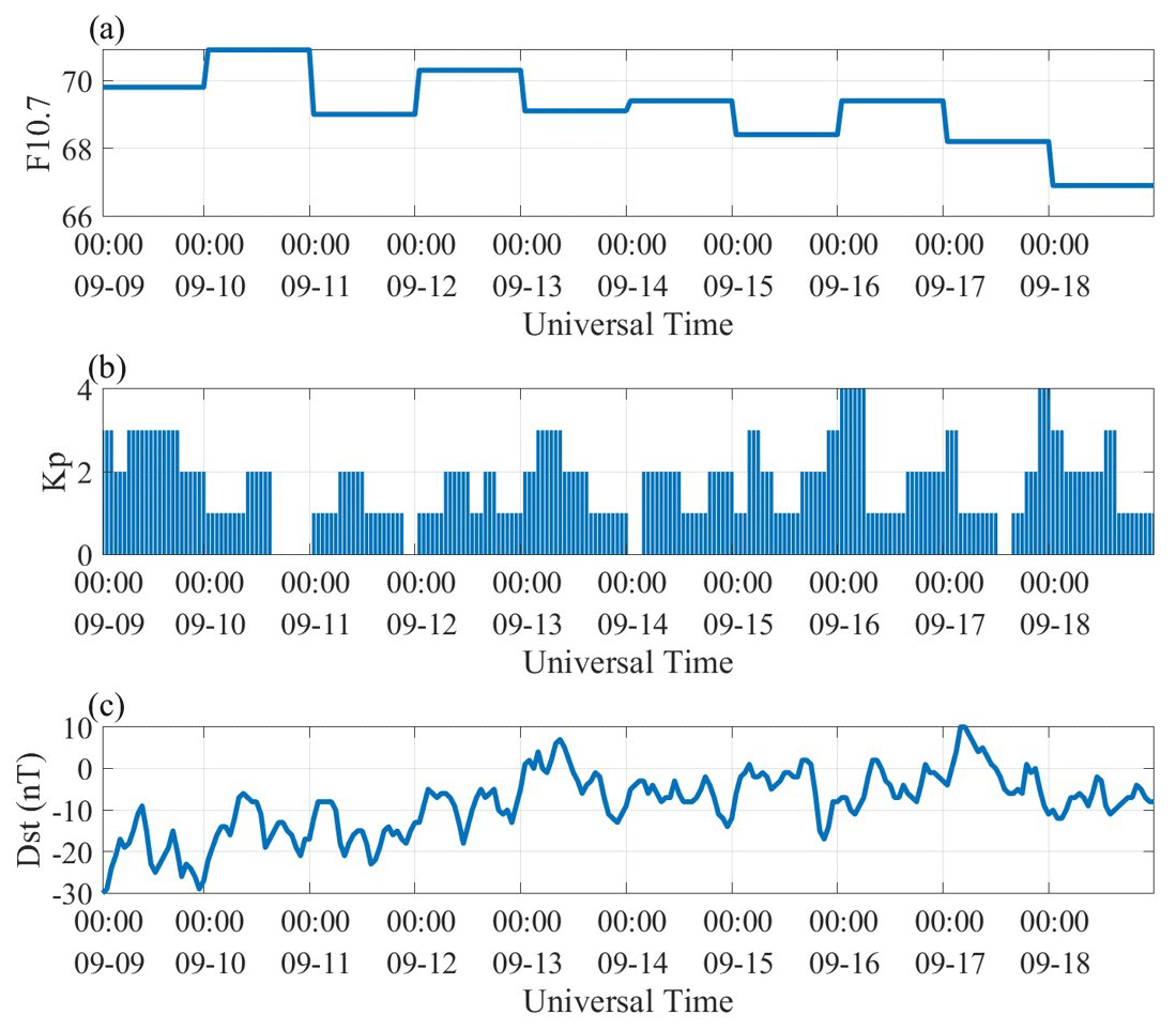
Figure 1 Space weather condition with F10.7 (a), Kp (b), and Dst (c) from 20190909 to 20190918. The LEO satellite receiver data in three MetOp satellites are selected from the CDAAC.

In previous studies, many factors affected the stability of ground-based GNSS receiver DCB, such as the quality of the orbit and observation data, space weather, the receiver type, antenna type, receiver hardware version, and receiver environment, especially the temperature (Zhang and Teunissen, 2015; Xue et al., 2016a, b; Li et al., 2017; Choi and Lee, 2018; Zha et al., 2019). By analyzing the receiver DCB of the BeiDou Navigation Satellite System (BDS) and Galileo satellite navigation system, it was found that the receiver type has no obvious relationship with the stability of the receiver DCB (Xue et al., 2016a, b; Li et al., 2018). But in the stability analysis of GPS receiver DCB, Choi and Lee (2018) found the type of receiver and antenna have a certain influence. Meanwhile, they also found that, after the receiver hardware version is replaced, the receiver DCB value will change significantly for the receiver DCB of GPS, BDS, Galileo, and other systems (Choi and Lee, 2018). There existed a strong linear correlation between the estimated receiver DCB and measured temperature values (Zha et al., 2019). On ground-based receivers, the standard deviation (SD) of some receiver DCBs can reach 1–2 ns (Wang et al., 2020). In space environments, when LEO satellites are moving, the temperature can change greatly, which may cause great instability in the LEO satellite GPS receiver DCB. An error of up to 8 TECU may affect the computed DCB during periods of strong solar activity. The estimated DCB may have an accuracy of about 3 TECU for low solar activity. In comparison to the receiver DCB, the satellite DCB is more than 10 times smaller (Conte et al., 2011). Furthermore, Kao et al. (2013) claimed that estimating errors rather than DCB changes are to blame for some of the bigger daily deviations in receiver DCBs. Various data processing techniques will result in various estimation mistakes. For some locations, smoothed and unsmoothed observations show DCB discrepancies of up to 6–8 TECU.

The Meteorological Operational (MetOp) satellites are in sun-synchronous near-circular orbit, and the ascending altitude is from 796 km to 844 km (Maybeck, 1982). The MetOp mission consists of three satellites in orbit, and the height of the satellites is about 817 km. The MetOp mission is considered the first step for the Earth observation space segment of the Global Monitoring for Environment and Security (GMES) initiative. The COSMIC Data Analysis and Archive Center (CDAAC) offers orbital data, approximated LEO satellite receiver DCB data, and dual-frequency GPS observation data aboard LEO satellites. Based on the local spherically symmetric assumption, the CDAAC uses geometric mapping functions and the local spherical symmetry to determine the receiver DCB (Yue et al., 2011), whose accuracy is about 1–2 TECU. The three MetOp satellites data are available from 20190714 to 20211127. However, the MetOp satellite receiver DCB is rarely studied, particularly in a short period.

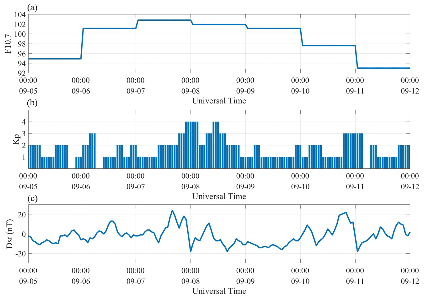
Figure 2 Space weather condition with F10.7 (a), Kp (b), and Dst (c) from 20210905 to 20210911. Unfortunately, the CDAAC does not have the LEO satellite receiver DCB value in this period, which is also a problem for MetOp satellites.

In this paper, daily and hourly DCBs of MetOp satellite receivers are estimated using the spherical harmonic function (SHF) and the local spherical symmetry (LSS) assumption, which are further evaluated and compared with the DCB products provided by the CDAAC. The MetOp data, local spherical symmetry assumption, and spherical harmonic function are introduced in Sect. 2. The results and analysis are presented in Sect. 3. In Sect. 4, the discussions are presented, and the conclusion is given in Sect. 5.

2 Data and methods

This part introduces the data used and provides details on the LSS assumption and SHF method.

2.1 LEO data

LEO satellites are easily affected by space weather. In order to reduce this effect and calculate the DCBs, a chosen period must satisfy the following conditions:

1. LEO observation data, the LEO satellites, and GPS satellite orbit data are available.

2. The observation period is as long as possible.

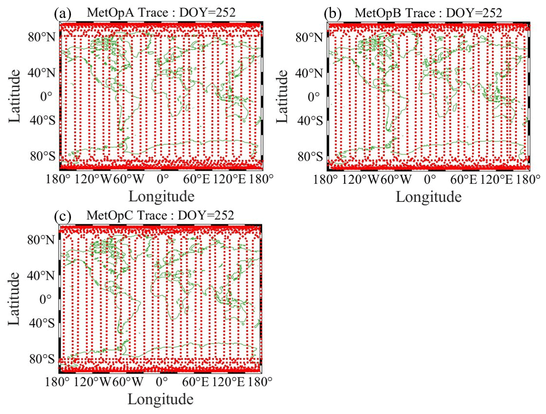
Figure 3 Satellite traces of MetOpA (a), MetOpB (b), and MetOpC (c) on day of the year (DOY) 252, in 2019.

The time periods from 9 September 2019 (day of the year 252) to 18 September 2019 (day of the year 261) and from 5 September 2021 (day of the year 248) to 11 September 2021 (day of the year 254) have been chosen. Figure 1 shows the solar activity and geomagnetic index during this time period. The F10.7 is under 80, the Dst is above −30 nT, and Kp is under 4, which indicated in this period that the geomagnetic condition is calm and that the solar activity is not quite active. The same concept also applies to Fig. 2 during the solar active period, as was previously mentioned. The range of F10.7 is 92–104, which suggests that this is a solar active period (https://www.sws.bom.gov.au/Educational/1/2/4, last access: 10 November 2023). Figure 3 illustrates the orbital paths of the three LEO satellites, and their period of motion is 1.68 h.

2.2 Slant total electron content (STEC) estimation from GNSS

The Receiver Independent Exchange Format (RINEX) is used to record carrier phase and pseudo-range measurements for GNSS. The pseudo-range and carrier phase observation equations for GPS are shown below (Jin et al., 2012):

$$\begin{array}{}\text{(1)}& {\displaystyle }\begin{array}{rl}{P}_{k,j}^i=& {\mathit{\rho }}_{\mathrm{0},j}^i+d_{\text{ion},k,j}^i+d_{\text{trop},k,j}^i+c\left({\mathit{\tau }}^{\mathrm{i}}-{\mathit{\tau }}_{\mathrm{j}}\right)\\ & +d_k^i+d_{k,j}+{\mathit{\epsilon }}_{P,k,j}^i,\end{array}\text{(2)}& {\displaystyle }\begin{array}{rl}{L}_{k,j}^i=& {\mathit{\rho }}_{\mathrm{0},j}^i-d_{\text{ion},k,j}^i+d_{\text{trop},k,j}^i+c\left({\mathit{\tau }}^{\mathrm{i}}-{\mathit{\tau }}_{\mathrm{j}}\right)\\ & -\mathit{\lambda }\left(b_{k,j}^i+N_{k,j}^i\right)+{\mathit{\epsilon }}_{L,k,j}^i,\end{array}\end{array}$$

where P and L are the GPS pseudo-range and phase measurement, respectively; ρ is the distance between the GPS satellite and GPS receiver; d_ion and d_trop are ionospheric and tropospheric delays, respectively; c is the speed of light in vacuum environment; τⁱ and τ_j are the satellite and receiver clock errors, separately; d is the code delays for the satellite and receiver biases; N is the ambiguity of the carrier phase; and ε is the other error in the GPS measurement. The phase advance of the satellite and receiver instrument biases can be represented by b.

The frequency is denoted by the subscript k (1, 2), the GPS receiver's sequence number is denoted by the subscript j, and the GPS satellite's sequence number is denoted by the superscript i. The ionospheric delays can be calculated from dual-frequency GPS measurements (f_L1=1575.42 MHz, f_L2=1227.60 MHz), with the following equations:

$$\begin{array}{}\text{(3)}& {\displaystyle }{P}_{\mathrm{4}}=P_{\mathrm{1}.j}^i-P_{\mathrm{2}.j}^i=d_{\text{ion},\mathrm{1},j}^i-d_{\text{ion},\mathrm{2},j}^i+{\mathrm{DCB}}^i+{\mathrm{DCB}}_j,\text{(4)}& {\displaystyle }\begin{array}{rl}{L}_{\mathrm{4}}=& L_{\mathrm{1}.j}^i-L_{\mathrm{2}.j}^i=-\left(d_{\text{ion},\mathrm{1},j}^i-d_{\text{ion},\mathrm{2},j}^i\right)\\ & -\mathit{\lambda }\left(N_{\mathrm{1},j}^i-N_{\mathrm{2},j}^i\right),\end{array}\end{array}$$

where ${\mathrm{DCB}}^i=d_{\mathrm{1}}^i-d_{\mathrm{2}}^i$ and ${\mathrm{DCB}}_j=d_{\mathrm{1},j}-d_{\mathrm{2},j}$ stand for the differential code biases of the satellites and differential code biases of the receivers, respectively.

Due to the high noise in the pseudo-range observations, P₄, the carrier phases are used to smooth the pseudo-range. The P_4,sm is expressed after smoothing as follows:

$$\begin{array}{}\text{(5)}& P_{\mathrm{4},\text{sm}}={\mathit{\omega }}_t{P}_{\mathrm{4}}\left(t\right)+(\mathrm{1}-{\mathit{\omega }}_t)P_{\mathrm{4},\text{prd}}\left(t\right)(t>\mathrm{1}),\end{array}$$

where t stands for the epoch number, ω_t is the weight factor related to epoch (Yuan et al., 2021), and

$$\begin{array}{}\text{(6)}& P_{\mathrm{4},\text{prd}}=P_{\mathrm{4},\text{sm}}(t-\mathrm{1})+\left(L_{\mathrm{4}}\right(t)-L_{\mathrm{4}}(t-\mathrm{1}\left)\right)(t>\mathrm{1}).\end{array}$$

The following function is an expression for the ionospheric delay:

$$\begin{array}{}\text{(7)}& d_{\text{ion}}={\displaystyle \frac{\mathrm{40.3}}{f^{\mathrm{2}}}}\mathrm{STEC},\end{array}$$

where f stands the frequency of the carrier, and STEC stands for the slant total electron content.

By replacing P₄ by P_4,sm, we can get the following function:

$$\begin{array}{}\text{(8)}& P_{\mathrm{4},\text{sm}}=\mathrm{40.3}\left({\displaystyle \frac{\mathrm{1}}{f_{\mathrm{1}}^{\mathrm{2}}}}-{\displaystyle \frac{\mathrm{1}}{f_{\mathrm{2}}^{\mathrm{2}}}}\right)\mathrm{STEC}+{\mathrm{DCB}}^i+{\mathrm{DCB}}_j.\end{array}$$

Combining Eqs. (7) and (8), the STEC from GNSS dual-frequency observations can be calculated as follow:

$$\begin{array}{}\text{(9)}& \mathrm{STEC}=-{\displaystyle \frac{f_{\mathrm{1}}^{\mathrm{2}}{f}_{\mathrm{2}}^{\mathrm{2}}}{\mathrm{40.3}\left(f_{\mathrm{1}}^{\mathrm{2}}-f_{\mathrm{2}}^{\mathrm{2}}\right)}}(P_{\mathrm{4},\text{sm}}-c\cdot {\mathrm{DCB}}^i-c\cdot {\mathrm{DCB}}_j),\end{array}$$

where the DCB unit is time.

2.3 Mapping function

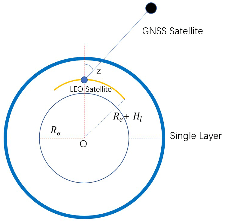
The mapping function (MF) can convert STEC to VTEC. Compared with the single-layer MF used by ground-based observations (Zhong et al., 2016), the Foelsche and Kirchengast (2002) (denoted F&K) geometric MF, whose geometric relation is shown in Fig. 4, has a more reasonable performance of STEC and VTEC conversion for the GPS-LEO link. The F&K geometric MF (Schaer et al., 1999) is expressed as

$$\begin{array}{}\text{(10)}& {\displaystyle }\mathrm{VTEC}=\mathrm{MF}\left(z\right)\cdot \mathrm{STEC},\text{(11)}& {\displaystyle }{M}_{F\text{ and }K}\left(z\right)={\displaystyle \frac{\mathrm{1}+R}{\cos z+\sqrt{R^{\mathrm{2}}-(\sin z{)}^{\mathrm{2}}}}},\text{(12)}& {\displaystyle }R={\displaystyle \frac{R_{\mathrm{e}}+H_{\mathrm{p}}}{R_{\mathrm{e}}+H_{\mathrm{l}}}},\end{array}$$

where z refers to the zenith angle, R_e is the radius of the Earth, H_l is the orbit altitude of LEO satellites, and H_p is the altitude of the single layer of the ionospheric pierce point (IPP).

Figure 4 F&K geometric MF.

2.4 Spherical harmonic function

The spherical harmonic function (SHF) is an easy way to establish a global VTEC map. The VTEC can be described as follows (Liu et al., 2020):

$$\begin{array}{}\text{(13)}& \begin{array}{rl}E(\mathit{\beta },s)=& \sum _{n=\mathrm{0}}^{n_{max}}\sum _{m=\mathrm{0}}^n{\stackrel{\mathrm{̃}}{P}}_{\text{nm}}\left(\sin \right(\mathit{\beta }\left)\right)\\ & \times \left(a_{\text{nm}}\cos \right(\mathrm{ms})+b_{\text{nm}}\sin (\mathrm{ms}\left)\right),\end{array}\end{array}$$

where β is the geocentric latitude of the IPP, s is the longitude of the IPP, a_nm and b_nm are the worldwide or regional ionosphere model coefficients, and ${\stackrel{\mathrm{̃}}{P}}_{\text{nm}}$ represents normalized Legendre polynomials.

The following equation can be established using Eqs. (12) and (13):

$$\begin{array}{}\text{(14)}& \begin{array}{rl}& \sum _{n=\mathrm{0}}^{n_{max}}\sum _{m=\mathrm{0}}^n{\stackrel{\mathrm{̃}}{P}}_{\text{nm}}\left(\sin \right(\mathit{\beta }\left)\right)\left(a_{\text{nm}}\cos \right(\mathrm{ms})+b_{\text{nm}}\sin (\mathrm{ms}\left)\right)=\\ & \cos \left(\text{arcsin}\left({\displaystyle \frac{R}{R+H}}\sin \left(\mathit{\alpha }z\right)\right)\right)\\ & \times \left(-{\displaystyle \frac{f_{\mathrm{1}}^{\mathrm{2}}{f}_{\mathrm{2}}^{\mathrm{2}}}{\mathrm{40.3}\left(f_{\mathrm{1}}^{\mathrm{2}}-f_{\mathrm{2}}^{\mathrm{2}}\right)}}\left(P_{\mathrm{4},\text{sm}}-c{\mathrm{DCB}}^i-c{\mathrm{DCB}}_j\right)\right),\end{array}\end{array}$$

The order of the spherical harmonic expansion depends on the area. Here, a set of ionospheric coefficients every 4 h is set based on the amount of collected data. In this paper, the order is set to be eight.

2.5 Local spherical symmetry assumption method

If the ionosphere is assumed to be locally spherically symmetric, then the local spherical symmetry (LSS) assumption equation for a given observation epoch can be written as follows with n GPS satellites observed simultaneously by the onboard GPS receiver:

$$\begin{array}{}\text{(15)}& \begin{array}{rl}& {\left(\begin{array}{c}{P}^{\mathrm{1}}-c\cdot {\mathrm{DCB}}^{\mathrm{1}}\\ P^{\mathrm{2}}-c\cdot {\mathrm{DCB}}^{\mathrm{2}}\\ \mathrm{⋮}\\ P^n-c\cdot {\mathrm{DCB}}^n\end{array}\right)}_{n\cdot \mathrm{1}}={\left(\begin{array}{cccc}{\mathrm{MF}}^{\mathrm{1}}& \mathrm{1}& \mathrm{0}& \mathrm{0}\\ {\mathrm{MF}}^{\mathrm{2}}& \mathrm{0}& \mathrm{1}& \mathrm{0}\\ \mathrm{⋮}& \mathrm{⋮}& \mathrm{⋮}& \mathrm{⋮}\\ {\mathrm{MF}}^n& \mathrm{0}& \mathrm{0}& \mathrm{1}\end{array}\right)}_{n\cdot \mathrm{4}}\\ & \cdot {\left(\begin{array}{c}\mathrm{VTEC}\\ {\mathrm{DCB}}_A\\ {\mathrm{DCB}}_B\\ {\mathrm{DCB}}_C\end{array}\right)}_{\mathrm{4}\cdot \mathrm{1}},\end{array}\end{array}$$

where MF is the mapping function. For the accuracy of calculation, the weighting is set related to the GPS satellites elevation.

Using the SHF method or LSS assumption, LEO receiver DCB and ionospheric coefficients or VTEC can be estimated by the least square method. Although GPS DCB and LEO satellite DCB can be estimated at the same time (because the number of MetOp satellites is three), GPS DCB data from the Deutsches Zentrum für Luft- und Raumfahrt (DLR) is used to reduce the number of unknown parameters to ensure accurate estimation of LEO satellite DCB.

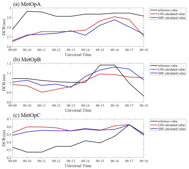
Figure 5 DCB sequence of MetOp satellite GPS receivers from 9 to 18 September 2019. The black line represents the receiver DCB provided by the CDAAC, the red line represents the receiver DCB estimated through LSS, and the blue line is the receiver DCB estimated through SHF.

2.6 Error estimation method

The error is represented by SD and RMSE in this article. RMSE, which measures how much the measured data deviate from the true value, is the square root of the ratio of the variation between the observed value and the true value to the number of observations N. A lower value denotes higher precision. If a CDAAC reference is available, the function below can be used to calculate RMSE.

$$\begin{array}{}\text{(16)}& X_{\text{RMSE}}=\sqrt{{\displaystyle \frac{{\sum }_{i=\mathrm{1}}^N(X_{\text{cal},i}-X_{\text{reference},i}{)}^{\mathrm{2}}}{N}}},\end{array}$$

where N is equal to 24 for 1 d estimation data, X_cal is the calculated value, and X_reference is the reference from the CDAAC.

The average square of the discrepancy between each sample value and the mean of all sample values is the variance. The steadier the value of X is, the lower the deviation is. The mathematical square root of the variance is called SD. It may also reflect a dataset's degree of dispersion. The SD is used in the absence of a reference value and can be calculated using Eq. (17).

$$\begin{array}{}\text{(17)}& X_{\text{SD}}=\sqrt{{\displaystyle \frac{{\sum }_{i=\mathrm{1}}^N(X_{\text{cal},i}-X_{\text{mean}}{)}^{\mathrm{2}}}{N}}},\end{array}$$

where X_mean is the mean value in the 1 d calculation.

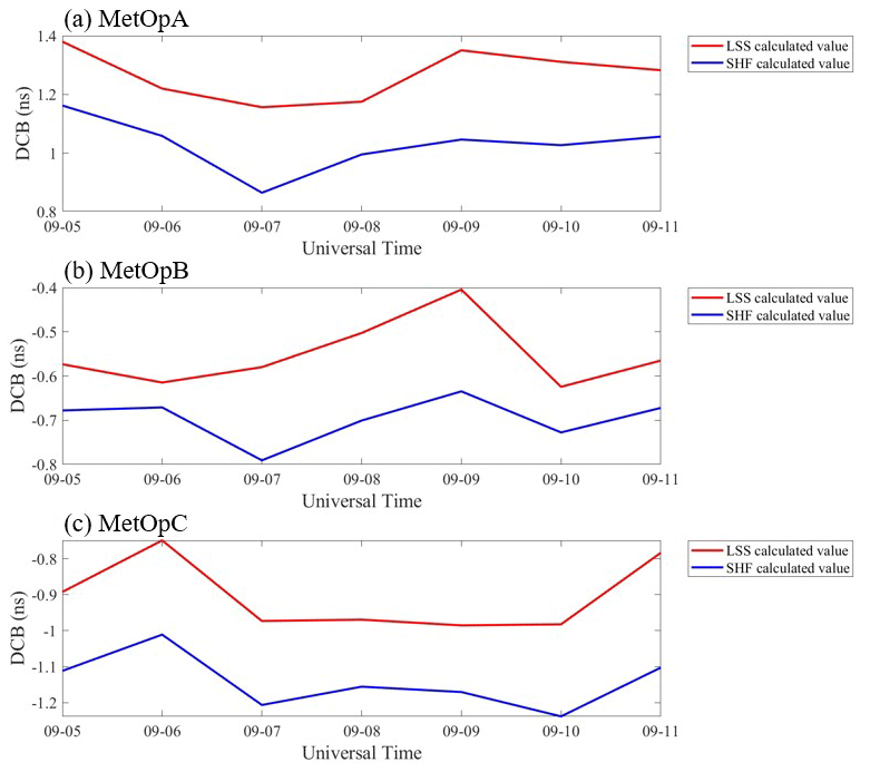
Figure 6 DCB sequence of MetOp satellite GPS receivers from 5 to 11 September 2021. The red line represents the receiver DCB estimated through LSS, and the blue line is the receiver DCB estimated through SHF.

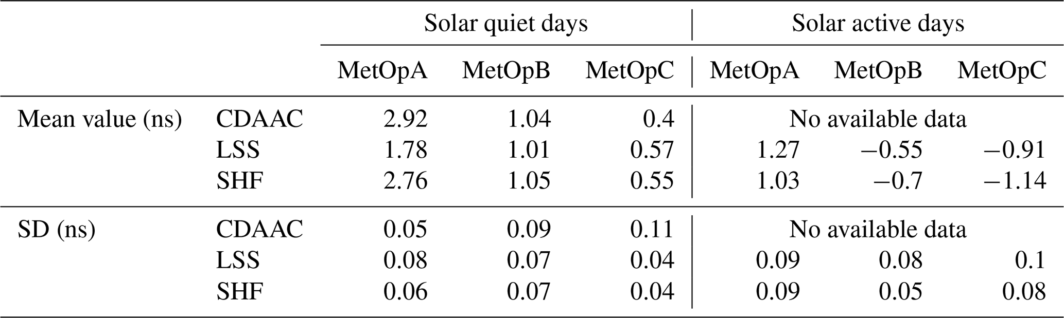
Table 1 Error analysis for different LEO satellites and different data source.

3 Results and analysis

3.1 Daily DCB estimation

First, the DCB is assumed as constant in a day, and the daily DCB estimation values for different time periods are estimated and shown in Figs. 5 and 6. The reference values are provided by the CDAAC. When focusing on solar quiet days, the results of MetOpA are underestimated. The results for MetOpB are occasionally overstated and occasionally underestimated. Most of the calculated results are overestimated for MetOpC. But the average error absolute value for the two methods is within 0.17 ns for the LSS assumption and within 0.16 ns for the SHF method. The absolute value of the mean error of MetOpB is the smallest among the three satellites. Although there are some differences in numerical values, the trend shows consistency. Unfortunately, there are no reference values for solar active days. Fig. 6 provides the calculated values from LSS and SHF. The average error absolute values between the two methods are within 0.04 and 0.24 ns for solar quiet days and solar active days, respectively. Within the solar quiet days, the reference value of DCB is quite stable, and the SD is within 0.11 ns. As for the estimation result from the LSS assumption, the calculated DCB SD is within 0.08 ns with respect to the reference value. The results of the SHF method demonstrate that the computed DCB standard deviation is within 0.07 ns. During the solar active days, the SD of the LSS-calculated DCB is within 0.10 ns, and the SD of the SHF-calculated DCB is within 0.09 ns. Some error analysis results are provided in Table 1 in detail.

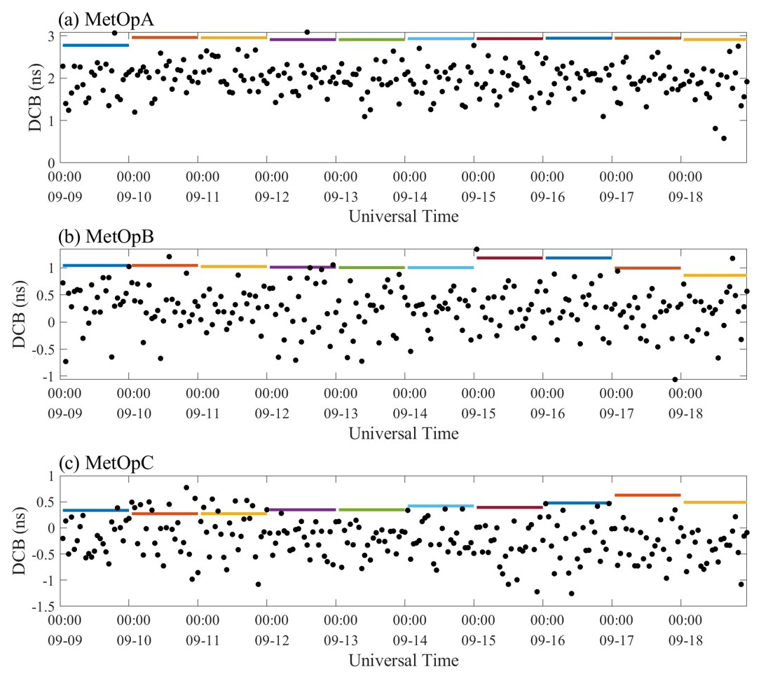
Figure 7 Distribution of DCB time series. The lines are the reference value of MetOpA, MetOpB, and MetOpC from the CDAAC, and the scatters are the calculated DCB based on the LSS method. Different colors of lines represent different days for reference values from the CDAAC.

Both approaches are excellent within the allowable error range, as can be seen from the study and comparison above. And both independent methods can obtain consistent receiver DCB results with respect to the CDAAC. The results of the study also clearly support the reliable MetOp receiver DCB values offered by the CDAAC. Besides, there are some differences between the estimated results of the two methods and the reference values, which may be due to the method error.

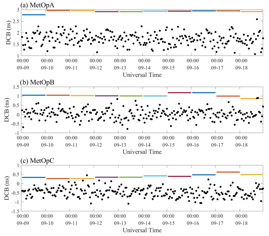
Figure 8 Distribution of DCB time series. The lines are the reference value of MetOpA, MetOpB, and MetOpC from the CDAAC, and the scatters are the calculated value by the SHF method. Different colors of lines represent different day reference values from the CDAAC.

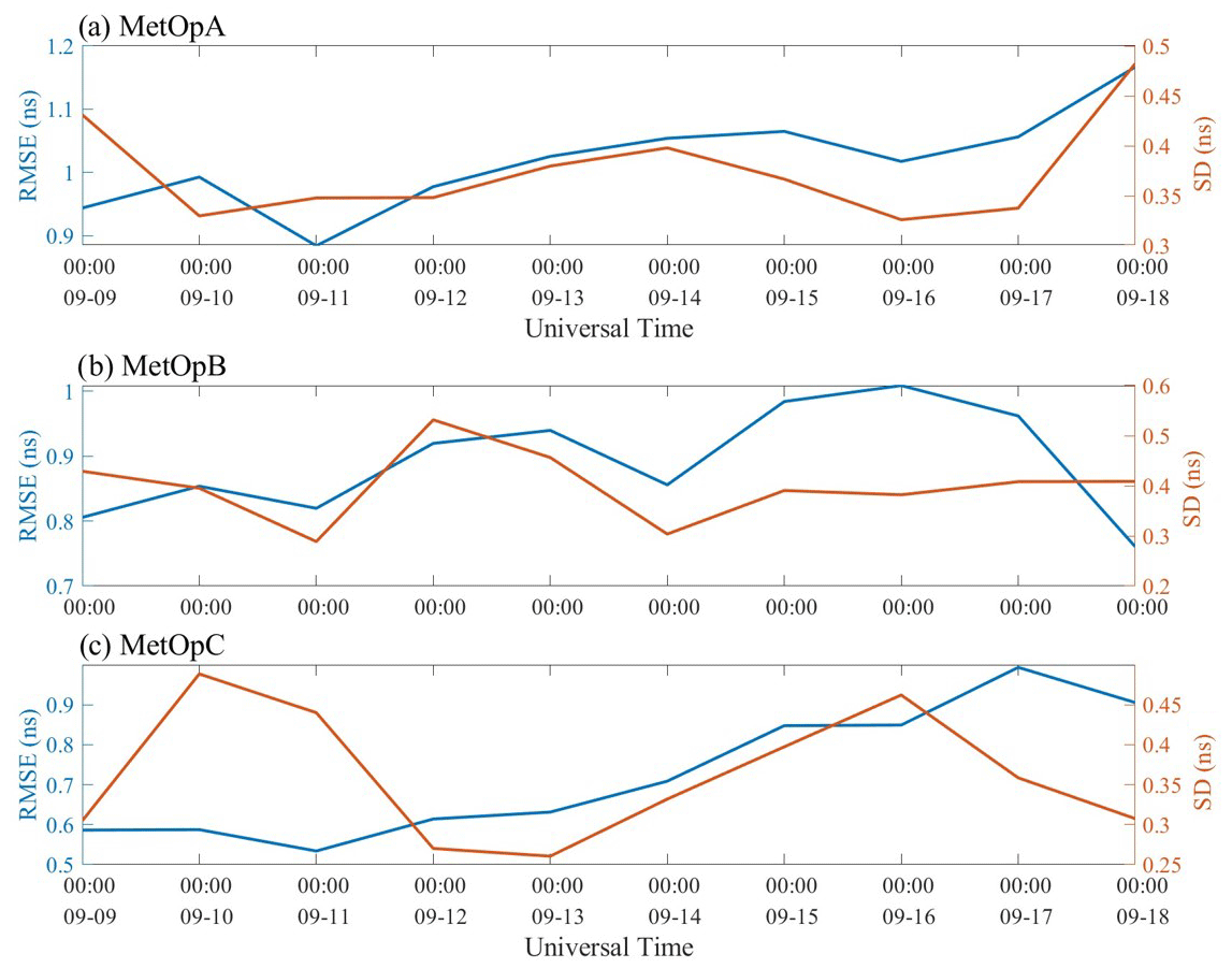
Figure 9 RMSE and SD of DCB from the LSS assumption for MetOpA, MetOpB, and MetOpC, respectively.

3.2 Hourly DCB estimation on solar quiet days

Hourly space-based GPS receiver DCBs are further estimated and shown in the figures below. Figure 7 illustrates the estimated hourly DCB from the LSS assumption, and Fig. 9 shows RMSE and SD of the hourly DCB estimation from the LSS assumption based on MetOpA, MetOpB, and MetOpC, respectively. For the estimation results based on the LSS assumptions, it can be found that the calculation results of MetOpA, MetOpB, and MetOpC range from 0.5 to 3.1 ns, from −1.1 to 1.5 ns, and from −1.3 to 0.7 ns, respectively. The RMSE ranges from 0.8 to 1.2 ns, from 0.7 to 1.1 ns, and from 0.5 to 1 ns, respectively. And the SD ranges from 0.3 to 0.5 ns, from 0.2 to 0.6 ns, and from 0.2 to 0.5 ns, respectively.

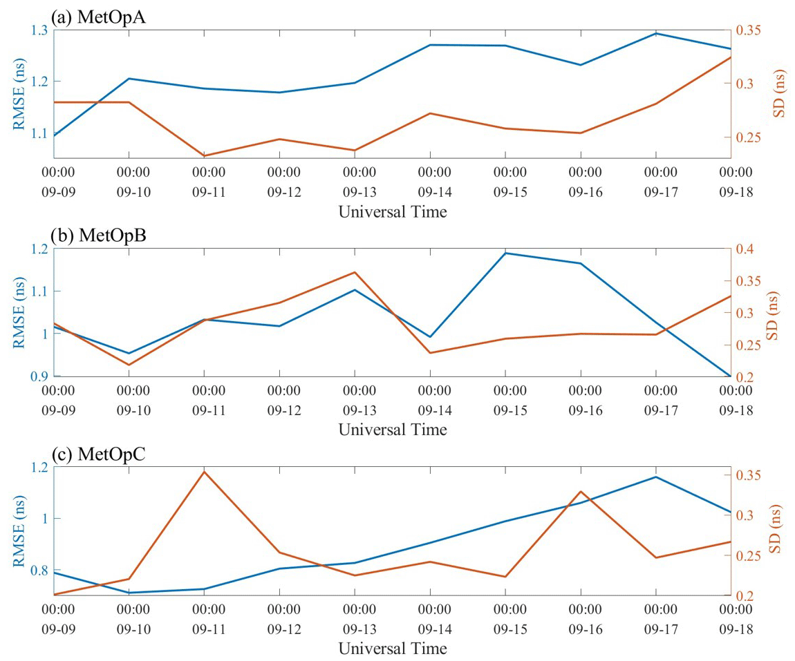
Figure 10 RMSE and SD of DCB calculated by SHF assumption for MetOpA, MetOpB, and MetOpC, respectively.

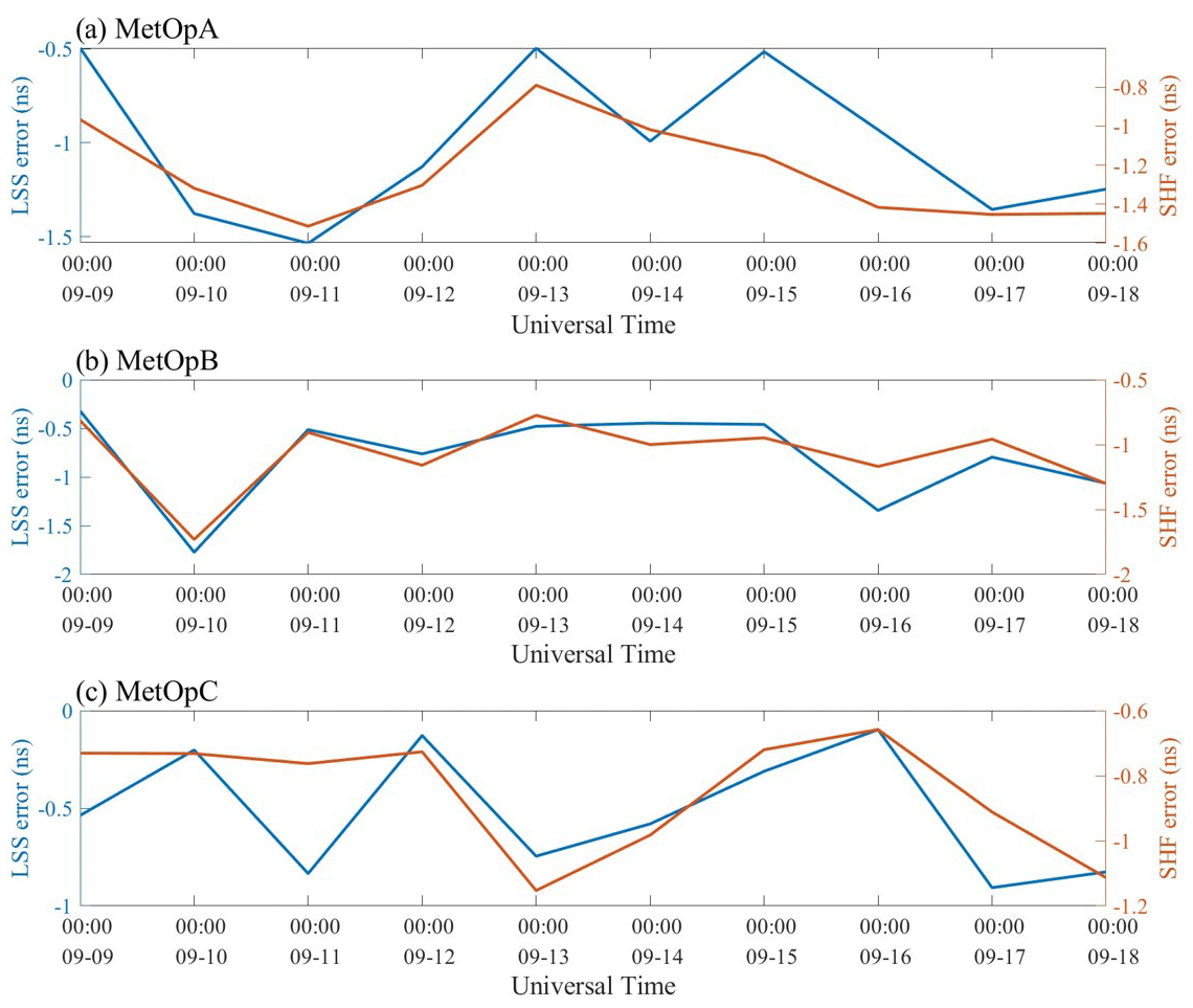
Figure 11 Mean absolute DCB value from the LSS assumption and SHF method for MetOpA, MetOpB, and MetOpC, respectively.

The estimated DCBs from the SHF method are shown in Fig. 8 as well as their RMSE and SD in Fig. 10. The calculation results show that the hourly DCBs have a certain change, while the calculated DCB is almost less than the CDAAC-provided reference value. For the estimation results from the SHF method, the calculation results of MetOpA, MetOpB, and MetOpC range from 1 to 2.7 ns, from −1 to 1 ns, and from −1.3 to 0.6 ns, respectively. The RMSE ranges from 1.1 to 1.3 ns, from 0.9 to 1.2 ns, and from 0.7 to 1.2 ns, respectively. And the SD is from 0.2 to 0.4 ns, from 0.2 to 0.4 ns, and from 0.2 to 0.4 ns, respectively.

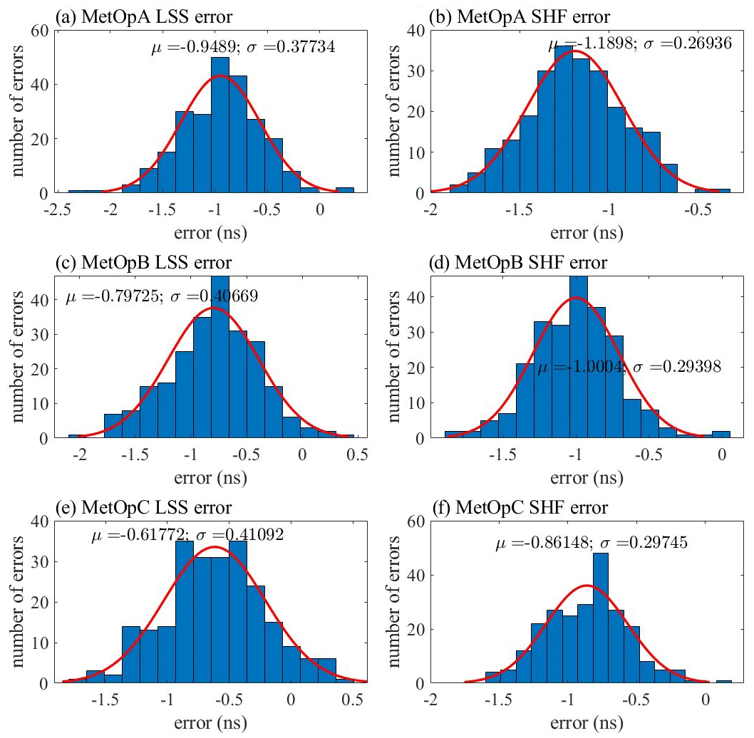
Figure 12 Frequency statistics of LSS and SHF error numbers with the LSS assumption and the SHF method based on MetOpA, MetOpB, and MetOpC data during 9–18 September 2019, respectively.

The average value of the error between DCBs from LSS and SHF and the given reference value in 1 d is shown in Fig. 11. With the LSS assumptions, the average daily error ranges from −1.8 to 0.3 ns, from −0.9 to −0.1 ns, and from −0.9 to −0.1 ns, respectively. And with the SHF method, the average daily error ranges from −1.5 to −0.7 ns, from −1.8 to −0.7 ns, and from −1.2 to −0.6 ns, respectively.

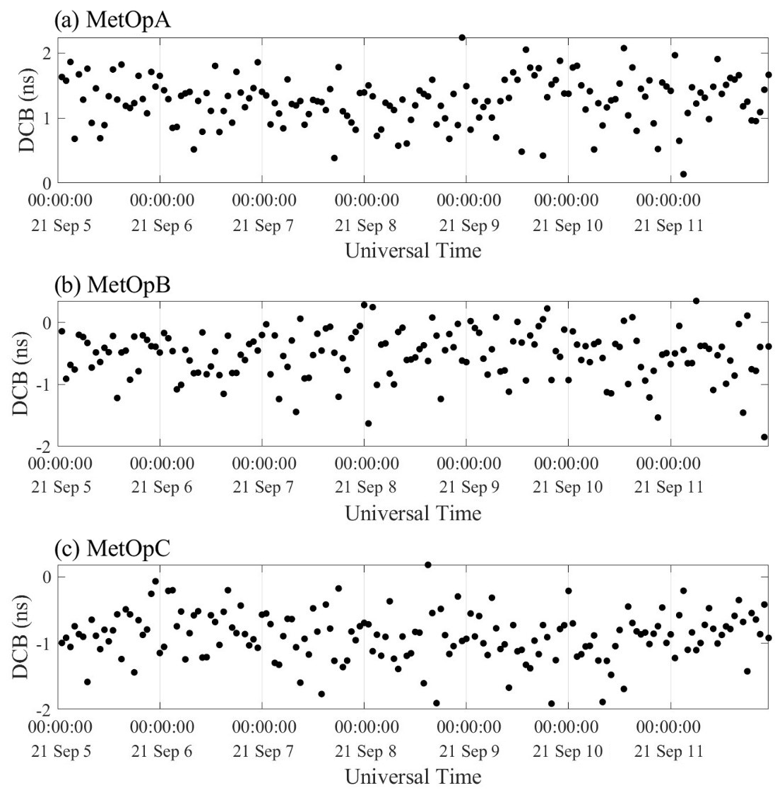
Figure 13 Distribution of DCB time series. The scatters are the calculated values by the LSS method (no reference value from the CDAAC).

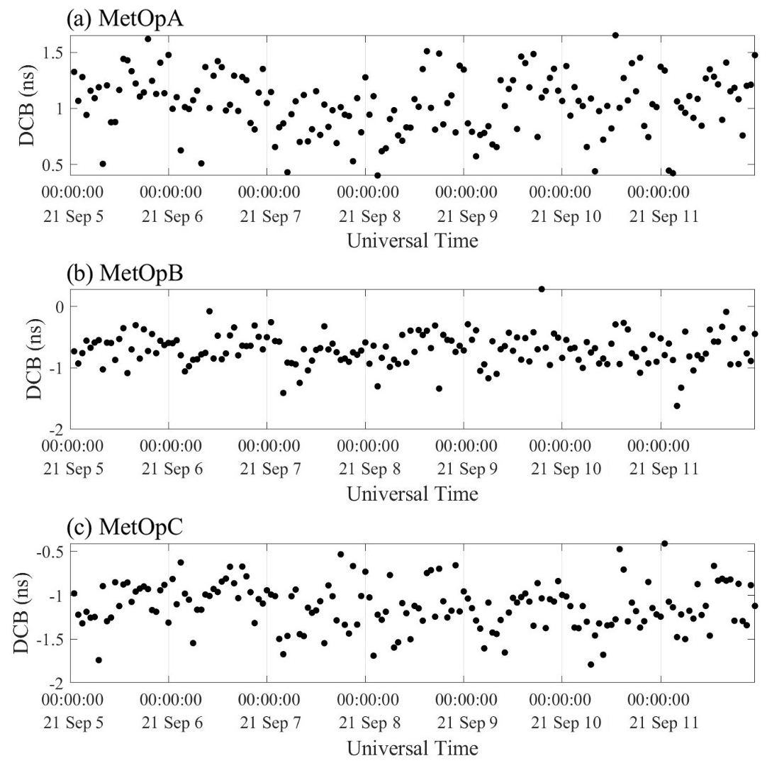
Figure 14 Distribution of DCB time series. The scatters are the calculated values by the SHF method (no reference value from the CDAAC).

Compared to LSS results, SHF outputs are still more precise and stable. But the SHF method requires a larger amount of data because there are more unknown parameters, which is also the limitation of this method. The main difference between the two calculation methods in calculating the daily DCB is not very large. But when calculating the hourly DCB, the results of the two methods are quite different. Therefore, when the amount of data is not enough, the LSS assumption is much better to calculate DCB. If the amount of data is enough, the SHF method is recommended. Hourly DCB time series shows high-frequency variations in 1 d. According to the statistical chart of frequency error analysis in Fig. 12, the error conforms to a normal distribution. Each μ value is under 0 ns, and the σ value is under 0.42 ns. This means that overall deviation exists, which may come from the method error. And the change of the calculated DCB should be attributed to the random error. In addition, the reference DCB from the CDAAC is not precise. Furthermore, the used MF can also cause an error between the calculated result and the reference value. Therefore, more errors and causes should be further studied and discussed in the future.

Figure 15 SD of DCB from the LSS method for MetOpA, MetOpB, and MetOpC, respectively.

Figure 16 SD of DCB from the SHF method for MetOpA, MetOpB, and MetOpC, respectively.

3.3 Hourly DCB estimation on solar active days

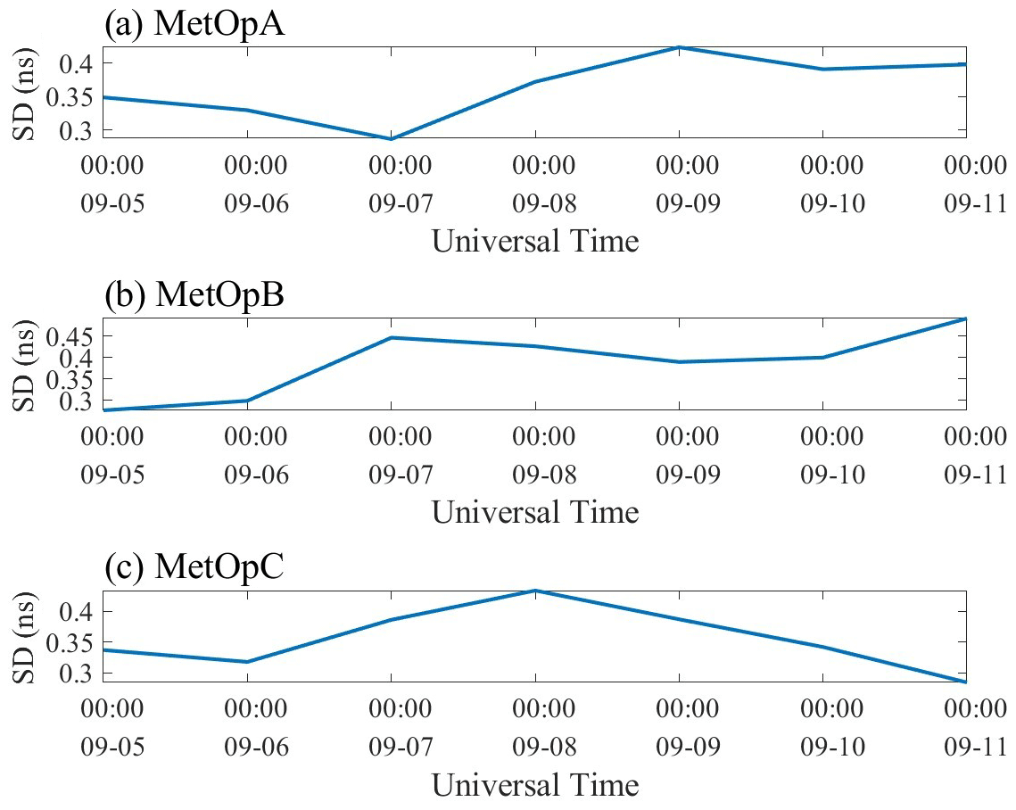
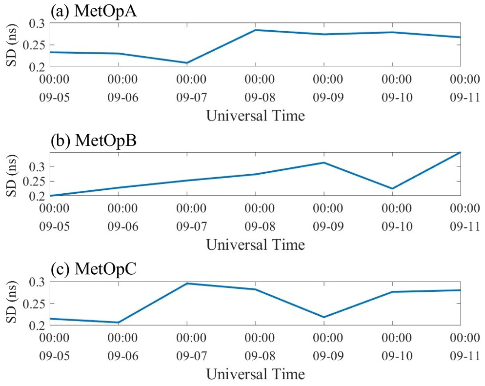
Hourly space-based LEO receiver DCBs are further calculated. As shown in Fig. 13, the daily fluctuation for MetOpA using the LSS approach is around 2 ns. Additionally, the highest fluctuations for MetOpB and MetOpC are approximately 2.2 ns. Figure 14 displays the DCB time series distribution of three LEO satellites with the SHF method; the changes in DCB are, respectively, 1.5, 1.2, and 1.2 ns. Unfortunately, there is no reference value at this time. Thus, the SD is computed. The SD of DCB from the LSS method is shown in Fig. 15 for MetOpA, MetOpB, and MetOpC, respectively. The range for MetOpA is from 0.28 to 0.43 ns. For MetOpB, the range is from 0.23 to 0.49 ns. And for MetOpC, the range is from 0.29 to 0.44 ns. Figure 16 shows the results of the SHF method. For MetOpA, the SD ranges from 0.21 to 0.28 ns. The range for MetOpB is between 0.2 and 0.35 ns. For MetOpC, the SD ranges from 0.21 to 0.29 ns.

4 Discussion

In this study, the LSS assumption and SHF method are used, respectively, to calculate the GPS receiver DCB of the LEO satellite in different solar conditions. The SD of the daily DCB calculated according to the LSS assumption for 9–18 September, 2020, is within 0.08 ns and is numerically smaller than the standard deviation of the reference value provided by the CDAAC. The absolute value of the average error is within 0.17 ns with respect to the DCB reference value. For solar active days, although there is no reference value from the CDAAC, the SD of the two methods can be introduced. And the results show that the SD is within 0.10 ns for the LSS assumption and is within 0.09 ns for the SHF method. The results show that LSS and SHF can be used to calculate daily DCBs.

The two methods are applied to calculate the hourly DCBs. For solar quiet days, the RMSE values of MetOpA, MetOpB, and MetOpC from LSS values are below 1.2, 1.1, and 1 ns, respectively. The SD values of MetOpA, MetOpB, and MetOpC are below 0.5, 0.6, and 0.5 ns, respectively. And the average daily error values of MetOpA, MetOpB, and MetOpC range from −1.8 to 0.3 ns, from −0.9 to −0.1 ns, and from −0.9 to −0.1 ns, respectively, which are higher than the daily estimation values. As for the RMSE of MetOpA, MetOpB, and MetOpC from the SHF method, they are less than 1.3, 1.2, and 1.2 ns, respectively. The MetOpA, MetOpB, and MetOpC SD values are below 0.35, 0.40, and 0.36 ns, respectively. The average daily error values of MetOpA, MetOpB, and MetOpC ranges from −1.5 to −0.7 ns, from −1.8 to −0.7 ns, and from −1.2 to −0.6 ns, respectively, which are also higher than the daily calculated DCBs. The fluctuations in 1 d of LSS and SHF are less than 2.24 and 1.62 ns, respectively. For solar active days, the SD of MetOpA, MetOpB, and MetOpC from LSS are, respectively, 0.37, 0.39, and 0.36 ns. And from SHF, the SDs of MetOpA, MetOpB, and MetOpC are less than 0.26, 0.27, and 0.26 ns, respectively. For the three LEO satellites, the fluctuations in 1 d of LSS and SHF are less than 2.20 and 1.53 ns, respectively. In other words, the changes of DCBs on solar active days and solar quiet days are similar. However, the DCBs are more stable in solar quiet days from Table 1, which means that the DCBs are influenced by the solar activity. Besides, the accuracy of hourly DCB estimation in solar active days cannot be debated, because the CDAAC did not provide references from 20210905–20210911.

Therefore, both methods can calculate reliable DCB results whether DCB is assumed as the same in 1 d or only in 1 h. And it is easy to find that compared to a day's data result, an hour's estimation error is much larger, which is the same as is found in the previous study (Li et al., 2017). The estimation accuracy of DCB is related to the amount of data as mentioned in the Introduction. This is also the reason why the calculation error of the daily estimations is smaller. Although the estimation results from the LSS assumption and the SHF method are slightly different, they are both stable and reliable, while the SHF method is a little more precise.

The hourly DCB estimation results show a certain change in the LEO satellite GPS receiver DCB. Although the error looks large, according to Choi and Lee (2018), the ground-based GNSS receiver DCBs can reach tens of nanoseconds. The SD of receiver DCB at all stations is below 2 ns, and Wang et al. (2020) also obtained the same results, implying that ground-based receiver DCB is less stable than satellite DCB. As previously indicated, the absolute error for the daily LEO satellite receiver DCB estimation is 3 TECU (or around 1.05 ns) (Zhang and Tang, 2014). Our hourly DCB estimation results for receivers on LEO satellites are accurate. Comparing the DCBs under the two scenarios, it is hard to demonstrate that the space weather can affect the results of DCB estimation. The DCB of the GPS receiver sometimes has significant intraday changes, which may be due to fluctuations in ambient temperature as introduced before. But in this study, the calculated hourly DCBs do not change greatly whether in solar calm days or in solar active days. Although the MetOp satellite can rotate around the Earth once every approximately 1.6 h and the space temperature changes apparently, the change of receiver DCB has little with the environment temperature because temperature control systems in the satellites exist. But the temperature inside the satellites related to the hourly change of ground-based DCB is unknown, because there is a lack of detailed data on the temperature inside the satellites. As in the previous study, it was found that the receiver CPU temperature also affected the DCB (Yue et al., 2011). Therefore, it might also be a reason for the change of LEO satellite GPS receiver DCB.

In addition, the antenna types, hardware, etc., may also cause DCB changes. But for MetOpA, MetOpB, and MetOpC, each LEO satellite uses same kind of antenna to receive signals. Therefore, it is excluded that the antenna type influences the calculation because the hardware conditions are unified. According to the statistical analysis of frequency errors in Fig. 12, the error conforms to a normal distribution, and the error may be the main reason for the change in the calculated DCB.

In data processing, this paper only estimates the receiver DCBs of three MetOp satellites. In the future, more satellites with similar heights should be used to estimate DCB, which can increase the data volume and improve the overall estimation accuracy (Choi and Lee, 2018).

5 Conclusion

In this study, the LSS assumption and the SHF method can both estimate the LEO satellite GPS receiver DCB well. It also provided verification for reference values from the CDAAC. Besides, the LEO satellite receiver DCBs provided by the CDAAC are missing on some dates, so we can also calculate the missing DCB value of the LEO satellite GPS receiver with these two methods. In addition, we also calculated and analyzed the hourly DCB through these two methods, and the main conclusions are summarized as follows:

1. The LSS assumption and the SHF method can both estimate the reliable LEO GPS receiver DCB well, whether DCB is assumed as the same or different in 1 d.

2. The SHF method is more stable and precise than the LSS assumption when compared with the reference value provided by the CDAAC. Also, the daily DCB estimation is more accurate and stable than the hourly DCB due to more data.

3. Hourly DCBs have changes in 1 d, but these can mainly attributed to random errors as these error time series conform a normal distribution. Satellite internal temperature may also be a possible reason to cause the change of hourly receiver DCB.