The m-dimensional spatial Nyquist limit using the wave telescope for larger numbers of spacecraft

Spacecraft constellations consisting of multiple satellites are becoming more and more interesting not only for commercial use but also for space science missions. The proposed and accepted scientific multi-satellite missions that will operate within Earth's magnetospheric environment, like HelioSwarm, require researchers to extend established methods for the analysis of multi-spacecraft data to more than four spacecraft. The wave telescope is one of those methods. It is used to detect waves and characterize turbulence from multi-point magnetic field data, by providing spectra in reciprocal position space. The wave telescope can be applied to an arbitrary number of spacecraft already. However, the exact limits of the detection for such cases are not known if the spacecraft, acting as sampling points, are irregularly spaced.

We extend the wave telescope technique to an arbitrary number of spatial dimensions and show how the characteristic upper detection limit in k space imposed by aliasing, the spatial Nyquist limit, behaves for irregularly spaced sampling points. This is done by analyzing wave telescope k-space spectra obtained from synthetic plane wave data in 1D up to 3D. As known from discrete Fourier transform methods, the spatial Nyquist limit can be expressed as the greatest common divisor in 1D. We extend this to arbitrary numbers of spatial dimensions and spacecraft. We show that the spatial Nyquist limit can be found by determining the shortest possible basis of the spacecraft distance vectors. This may be done using linear combination in position space and transforming the obtained shortest basis to k space. Alternatively, the shortest basis can be determined mathematically by applying the modified Lenstra–Lenstra–Lovász (MLLL) algorithm combined with a lattice enumeration algorithm. Thus, we give a generalized solution to the determination of the spatial Nyquist limit for arbitrary numbers of spacecraft and dimensions without any need of a priori knowledge of the measured data.

Additionally, we give first insights into the application to real-world data incorporating spacecraft position errors and minimizing k-space aliasing. As the wave telescope is an estimator for a multi-dimensional power spectrum substituting spatial Fourier transform, the results of this analysis can be applied to power spectral density estimation via Fourier transform or other methods making use of irregular sampling points. Therefore, our findings are also of interest to other fields of signal processing.

1 Introduction

The interaction of the solar wind with intrinsic planetary magnetic fields creates interaction regions like the magnetosheath or the foreshock region (e.g., Baumjohann and Treumann, 2012) that exhibit energy transport and transfer via turbulence or plasma waves (e.g., Narita, 2012). Multi-point measurements provided by the CLUSTER (Escoubet et al., 2001), THEMIS (Angelopoulos, 2008) and MMS (Burch et al., 2016) space missions have become a standard in Earth-bound plasma observations for more than 2 decades. They allow for the study of these processes and phenomena within a 3D picture.

However, especially with regard to turbulence, energy dissipation happens on different spatial and temporal scales (Frisch and Kolmogorov, 1995; Narita et al., 2006, 2011). Additionally, plasma waves and modes observed within terrestrial magnetospheric regions exhibit frequencies and wave vectors on different spatial scales (e.g., Borovsky and Valdivia, 2018), depending on plasma environmental conditions and the specific region. Thus, to understand these transfer processes as a whole, multi-scale observations on different spatial scales simultaneously are required. The HelioSwarm mission (Klein and Spence, 2021) with its nine spacecraft (S/C) to be launched in 2028 provides a unique possibility for such a multi-scale analysis. Furthermore, mission proposals such as the Plasma Observatory (Retino, 2021) demonstrate the current focus towards multi-scale multi-point missions.

For multi-point missions, different analysis techniques have been developed to use multi-point measurements. The wave telescope is an inversion technique to determine energy spectra that are dependent on both the frequency ω and the wave vector k. Thus, it enables us to identify dominant wave vector contributions in spatial magnetic field measurements, supporting the characterization and identification of plasma waves and turbulence phenomena (Motschmann et al., 1996; Narita et al., 2022). The wave telescope has been applied successfully to CLUSTER and MMS data among others (e.g., Glassmeier et al., 2001; Pinçon and Glassmeier, 2008; Narita et al., 2016). Its algorithm is able to handle an arbitrary number of multi-point measurements. However, when analyzing discrete data, analysis limits like the Nyquist limit are applicable. This applies in frequency space but also in wave vector space, the k space (Narita and Glassmeier, 2009). Hereafter, we call this limit in k space the spatial Nyquist limit. Working in 3D space, four equally spaced S/C are sufficient to determine the spatial Nyquist limit as known from solid-state physics and the concept of the Brillouin zone (Brillouin, 1930; Kittel, 1991). In this case, the number of required S/C n is just $n=m+\mathrm{1}$, where m is the number of spatial dimensions. However, if $n>m+\mathrm{1}$, an overdetermined equation system arises for determining the spatial Nyquist limit. In this case, the Nyquist limit determination is not trivial anymore. A zero-order approximation of the limit was recently provided by Zhang et al. (2021) for the wave telescope application.

Here, we derive a more precise formulation of the spatial Nyquist limit for an arbitrary number of S/C and dimensions using synthetic data models of multi-point measurements. In Sect. 2, a short recap of the wave telescope technique is given, extending the known formulae to arbitrary dimensions while focusing on the version used for the here-presented synthetic data models. Additionally, the known definitions of sampling restrictions, namely, the Nyquist limit in both time and space, are presented. Afterwards, Sect. 3 provides an introduction to what is already known about the (spatial) Nyquist limit for irregular sampling points – mostly in low-dimension problems from other fields of research – and, on the other hand, shows our extension to this current knowledge by our findings considering the wave telescope, large S/C numbers and also high-dimension problems. The mathematical generalization is formulated, and algorithms for the computation of the spatial Nyquist limit are shown. Section 4 then focuses on the generation and improvement of real-data spectra by incorporating position errors and making use of spectra of subsets of S/C. We conclude our results and provide an outlook on the possible applications of our findings to other research areas (Sect. 5).

2 Physical and mathematical basis

The following section provides the fundamentals of aliasing and its transfer to multi-dimensional reciprocal location space, namely, k space. The phenomenon of aliasing is a general one in the analysis of discrete signals, also in k space. Nevertheless, here we focus on its implications for the wave telescope technique, which will be introduced first before showing a general derivation of the aliasing limit in k space for regularly (evenly) spaced sampling points. Despite the focus on the wave telescope technique, the findings and consideration presented in this study regarding the aliasing in k space are of a general nature and can be applied to other spectrum estimation techniques.

2.1 The wave telescope technique for an arbitrary number of dimensions

The wave telescope technique enables the estimation of a wave-vector-dependent spectrum from a limited number of measurement points (Motschmann et al., 1996). The technique allows for the estimation of wave power in k space (Narita et al., 2022). It is based on the maximum-likelihood technique applied to seismic wave data (Capon et al., 1967; Capon, 1969), which was later extended to observations in the context of electromagnetic waves (Pinçon and Lefeuvre, 1991). Adaption to the use of magnetic field data with solenoidality as an additional constraint was provided by Motschmann et al. (1996). This wave telescope was introduced as a new analysis method for the CLUSTER mission. It uses Capon's minimum variance projection (Narita, 2019), also known as the minimum variance distortionless response (MVDR) estimator (Haykin, 1991; Toepfer et al., 2020). For a detailed derivation of the method, the reader is referred to the previously mentioned references. Here, we will just focus on the estimator itself for an arbitrary number of S/C n, based on the description in Motschmann et al. (1996). However, the dimension m is chosen arbitrarily. By dimension, we mean the considered number of vector components of the physical quantity, in our case the magnetic field. In this work, this number of dimensions is always chosen to be equal to the number of spatial dimensions. Thus m is at maximum 3.

Suppose that the magnetic field vector b(t,r) is sampled at the S/C positions ${\mathit{r}}_{\mathrm{1}},\mathrm{\dots },{\mathit{r}}_n$. The time resolution of magnetic field data shall be sufficient to allow for a Fourier transform in time (consider Eq. 9 below), delivering b(ω,r). An (m⋅n) column vector is introduced to combine all measurements:

$$\begin{array}{}\text{(1)}& \mathbf{B}\left(\mathit{\omega }\right)=\left(\begin{array}{c}\mathit{b}(\mathit{\omega },{\mathit{r}}_{\mathrm{1}})\\ \mathrm{⋮}\\ \mathit{b}(\mathit{\omega },{\mathit{r}}_n)\end{array}\right).\end{array}$$

With that, a data covariance matrix is defined by taking an ensemble average

$$\begin{array}{}\text{(2)}& \mathbf{M}=\langle \mathbf{B}\left(\mathit{\omega }\right){\mathbf{B}}^{†}\left(\mathit{\omega }\right)\rangle .\end{array}$$

This is a square matrix of size ($m\cdot n\times m\cdot n$), where † denotes the Hermitian transpose. To estimate this ensemble average from a time series of finite length, we divide the original time series interval into Q sub-intervals b_q(t) (Glassmeier et al., 2001). Fourier transformation in time of each sub-interval yields b_q(ω), which may then be condensed to B_q(ω), using Eq. (1). This procedure assumes stationarity and homogeneity of the time series analyzed. With this, the data matrix can be written as

$$\begin{array}{}\text{(3)}& \mathbf{M}={\displaystyle \frac{\mathrm{1}}{Q}}\sum _{q=\mathrm{1}}^Q{\mathbf{B}}_q\left(\mathit{\omega }\right){\mathbf{B}}_q^{†}\left(\mathit{\omega }\right).\end{array}$$

The number of sub-intervals should be chosen sufficiently large so as to minimize the random error compared to the estimate itself (cf. Bendat and Piersol, 1971). Thirty-two degrees of freedom are considered sufficient; that is, Q=16 (Glassmeier et al., 2001).

A model matrix H is introduced, representing the assumed model, which is in our case the plane wave assumption:

$$\begin{array}{}\text{(4)}& \mathbf{H}=\left(\begin{array}{c}{\mathbf{I}}_m{\mathrm{e}}^{i\mathit{k}{\mathit{r}}_{\mathrm{1}}}\\ \mathrm{⋮}\\ {\mathbf{I}}_m{\mathrm{e}}^{i\mathit{k}{\mathit{r}}_n}\end{array}\right),\end{array}$$

which is of the size ($m\cdot n\times m$), with I_m being the identity matrix of size m. Different underlying models can be chosen such as spherical waves (Constantinescu et al., 2006) or phase-shifted waves (Plaschke et al., 2008). With a plane wave model, the wave telescope technique can be interpreted as a power spectrum estimator substituting power spectral density estimation via a spatial Fourier transform (Motschmann et al., 1996; Plaschke et al., 2008; Narita and Glassmeier, 2009).

To guarantee the divergence-free nature of the magnetic field, a filter matrix can be introduced:

$$\begin{array}{}\text{(5)}& \mathbf{V}={\mathbf{I}}_m+{\displaystyle \frac{\mathit{k}}{\left|\mathit{k}\right|}}\otimes {\displaystyle \frac{\mathit{k}}{\left|\mathit{k}\right|}}={\mathbf{I}}_m+{\displaystyle \frac{\mathit{k}{\mathit{k}}^{\mathrm{T}}}{|\mathit{k}{|}^{\mathrm{2}}}},\end{array}$$

where ⊗ denotes the dyadic product. The spectral energy matrix P of size (m×m) is estimated via

$$\begin{array}{}\text{(6)}& \mathbf{P}={\left({\mathbf{V}}^{†}{\mathbf{H}}^{†}{\mathbf{M}}^{-\mathrm{1}}\mathbf{HV}\right)}^{-\mathrm{1}}.\end{array}$$

The spectral power P at a specific k is defined as the trace of the spectral energy matrix P:

$$\begin{array}{}\text{(7)}& P=\mathrm{tr}\left(\mathbf{P}\right).\end{array}$$

The determination of P requires the existence of M⁻¹. This may be achieved by applying so-called diagonal loading to the data matrix by adding artificial noise ${\mathit{\sigma }}_{\mathrm{d}}^{\mathrm{2}}$ such as described in further detail by Toepfer et al. (2020):

$$\begin{array}{}\text{(8)}& {\mathbf{M}}_{\mathrm{d}}=\mathbf{M}+{\mathbf{I}}_{m\cdot n}\cdot {\mathit{\sigma }}_{\mathrm{d}}^{\mathrm{2}}.\end{array}$$

For discrete data, this procedure provides a power estimate P for a specific wave vector k (input to the matrices H and V) and frequency ω (chosen when calculating M). To determine a full power spectrum, a scan of four-dimensional parameter space spanned by the three wave vector components and the frequency is required. As mentioned before, the time resolution is usually sufficiently high to provide spectral power estimates in the frequency domain by making use of a temporal Fourier transform.

Therefore, we focus on the limits for estimating the spatial power spectrum, that is, estimating the spectral power P(k) for a suitable range of wave vectors and at any given frequency. Thus, we will only chose one frequency to be analyzed – the frequency yielding maximum power when calculating an average temporal power spectral density. All input waves in the model cases will be at that specific frequency, allowing us to focus on k space alone.

2.2 Definition of the spatial Nyquist limit for regular sampling

For regularly (evenly) sampled discrete data, the sampling theorem (e.g., Nyquist, 1928; Shannon, 1949) states that to recover a signal of at maximum a frequency of f, a sampling frequency of at least f_s=2f is needed. This results in the Nyquist frequency $f_{\mathrm{Ny}}=\mathrm{1}/\left(\mathrm{2}\mathrm{\Delta }t\right)$ as an upper detection limit for waves or periodic structures, with $\mathrm{\Delta }t=\mathrm{1}/f_{\mathrm{s}}$ being the sampling step. When transforming a time series to the frequency domain, signals above the Nyquist frequency show aliasing. One of the most common transforms is the discrete Fourier transformation (DFT), which reads for a discrete time series b(t_j) (Eriksson, 1998) as

$$\begin{array}{}\text{(9)}& B\left(f_{\mathit{\gamma }}\right)={\displaystyle \frac{\mathrm{1}}{M}}\sum _{j=\mathrm{0}}^{M-\mathrm{1}}b\left(t_j\right)\cdot \exp (\mathrm{2}\mathit{\pi }i\cdot f_{\mathit{\gamma }}\cdot t_j)\end{array}$$

with the corresponding inverse discrete Fourier transform (IDFT) from frequency to time domain as

$$\begin{array}{}\text{(10)}& b\left(t_j\right)=\sum _{\mathit{\gamma }=\mathrm{0}}^{M-\mathrm{1}}B\left(f_{\mathit{\gamma }}\right)\cdot \exp (-\mathrm{2}\mathit{\pi }i\cdot f_{\mathit{\gamma }}\cdot t_j),\end{array}$$

where $f_{\mathit{\gamma }}=\mathit{\gamma }/(M\cdot \mathrm{\Delta }t)$ is the discrete frequency with $\mathit{\gamma }=\mathrm{0},\mathrm{1},\mathrm{\dots },M-\mathrm{1}$. In order to yield a spectrum, one normally estimates the power spectral density (PSD), which can be accomplished by a range of different methods. Nevertheless, here we want to focus on Fourier transform as an illustrative example with its two-sided PSD estimator (compare with Eriksson, 1998)

$$\begin{array}{}\text{(11)}& P_{\mathrm{DFT}}={\displaystyle \frac{M}{f_{\mathrm{s}}}}\left|B\right(f_{\mathit{\gamma }}){|}^{\mathrm{2}}.\end{array}$$

Aliasing can be seen both in the time domain and the frequency domain. When, for example, regularly sampling a sinusoidal wave of frequency f₀, any other sine with a frequency of f₀±gf_s can also perfectly fit to the time series (with g being an integer). The DFT spectrum P_DFT will thus show a periodicity with 2f_Ny. All frequencies from a range $\left(\right(l-\mathrm{1})f_{\mathrm{Ny}},(l+\mathrm{1}\left)f_{\mathrm{Ny}}\right]$ will also show up in every other range $\left(\right(q-\mathrm{1})f_{\mathrm{Ny}},(q+\mathrm{1}\left)f_{\mathrm{Ny}}\right]$ with l and q being even integers (Bretthorst, 2001; Kirchner, 2005). Thus, the spectrum in the frequency domain consists of a twofold spectrum: the original (true) spectrum and an aliased spectrum that is added to it. In the following, for simplicity, we will consider and implement in the simulations only frequencies (respectively wave vectors; see the next paragraph) within the true spectrum. This means, in approximation, that only the true spectrum in the range from 0 to the Nyquist frequency will be repeating indefinitely, and in the frequency range $-f_{\mathrm{Ny}}\le f\le f_{\mathrm{Ny}}$ the resulting Fourier spectrum is aliasing free. Signal contributions at frequencies above f_Ny (and below −f_Ny) show aliasing. For more detailed information on the basics of aliasing, the reader is referred to Kirchner (2005) and VanderPlas (2018).

The concept of aliasing and frequency domain periodicity can be directly transferred from frequency space to k space in general (Dunlop et al., 1988; Chanteur, 1998), in particular for the wave telescope (Neubauer and Glassmeier, 1990; Pinçon and Motschmann, 1998; Glassmeier et al., 2001; Narita and Glassmeier, 2009). This implies an analogue of the Nyquist frequency in k space: the spatial Nyquist limit k_Ny. However, there is a major difference when using the wave telescope technique. For a real time series, the power spectrum in the frequency domain is symmetric around 0 (Kirchner, 2005). The wave telescope, however, estimates a spatial Fourier transform of the complex data set B(ω) (Eq. 1). Thus, the spatial power spectrum obtained is not symmetric around 0. The full range from the negative to the positive spatial Nyquist limit needs to be considered.

In a first step to determine the spatial Nyquist limit, we have to establish the periodic k cell within reciprocal space. This periodic cell is spanned by a set of skewed linearly independent basis vectors k_i. These vectors are determined by the relation

$$\begin{array}{}\text{(12)}& \left(\begin{array}{c}{\mathit{d}}_{\mathrm{1}}^{\mathrm{T}}\\ \mathrm{⋮}\\ {\mathit{d}}_m^{\mathrm{T}}\end{array}\right)\cdot \left(\begin{array}{ccc}{\mathit{k}}_{\mathrm{1}}& \mathrm{\cdots }& {\mathit{k}}_m\end{array}\right)=\mathrm{2}\mathit{\pi }{\mathbf{I}}_m\end{array}$$

with $m\in \mathit{\{}\mathrm{1},\mathrm{2},\mathrm{3}\mathit{\}}$ and I_m being the identity matrix of size m (derived from Shmueli, 2008, and Souvignier, 2016, and references therein). We expect that the spacecraft span the whole dimension space and thus exclude degenerate cases where the basis vectors would not be linearly independent. Here, the spacecraft translation vectors d_i represent the difference between the position of an arbitrarily chosen reference spacecraft r₁ and all other spacecraft with position vectors r_i (i.e., the set of basis vectors k_i is not unique):

$$\begin{array}{}\text{(13)}& {\mathit{d}}_i={\mathit{r}}_{i+\mathrm{1}}-{\mathit{r}}_{\mathrm{1}},\end{array}$$

with $i=\mathrm{1},\mathrm{2},\mathrm{\dots },n-\mathrm{1}$ and n being the number of S/C. The d_i vectors represent column vectors of length m in position space; k_i represent column vectors of length m in reciprocal space. Note that for the case of regular sampling considered in this section $n=m+\mathrm{1}$.

Solving Eq. (12) yields the expressions for the basis vectors k_i of the periodic cell in different dimensions m. For a 1D situation (the translation vectors become scalars d_i),

$$\begin{array}{}\text{(14)}& k_{\mathrm{1}}={\displaystyle \frac{\mathrm{2}\mathit{\pi }}{d_{\mathrm{1}}}},\end{array}$$

and in 2D (Achar, 1986)

$$\begin{array}{}\text{(15)}& {\mathit{k}}_{\mathit{\alpha }}=\mathrm{2}\mathit{\pi }{\displaystyle \frac{|{\mathit{d}}_{\mathit{\beta }}{|}^{\mathrm{2}}{\mathit{d}}_{\mathit{\alpha }}-({\mathit{d}}_{\mathit{\alpha }}\cdot {\mathit{d}}_{\mathit{\beta }}){\mathit{d}}_{\mathit{\beta }}}{\left|{\mathit{d}}_{\mathit{\alpha }}{|}^{\mathrm{2}}\right|{\mathit{d}}_{\mathit{\beta }}{|}^{\mathrm{2}}-({\mathit{d}}_{\mathit{\alpha }}\cdot {\mathit{d}}_{\mathit{\beta }}{)}^{\mathrm{2}}}},\end{array}$$

with cyclic permutation of $\mathit{\alpha },\mathit{\beta }=\mathrm{1},\mathrm{2}$ leading to two vectors that span a parallelogram. For a 3D situation, these vectors read (e.g., Kittel, 1991) as

$$\begin{array}{}\text{(16)}& {\mathit{k}}_{\mathit{\mu }}=\mathrm{2}\mathit{\pi }{\displaystyle \frac{{\mathit{d}}_{\mathit{\nu }}\times {\mathit{d}}_{\mathit{\xi }}}{{\mathit{d}}_{\mathit{\mu }}\cdot ({\mathit{d}}_{\mathit{\nu }}\times {\mathit{d}}_{\mathit{\xi }})}},\end{array}$$

using cyclic permutation for $\mathit{\mu },\mathit{\nu },\mathit{\xi }=\mathrm{1},\mathrm{2},\mathrm{3}$.

As mentioned above, the vectors k_i define a confined structure in k space, the periodic cell. For the wave telescope, as abovementioned, one has to consider the spectrum from negative to positive spatial Nyquist limit. Thus, we can define the spatial Nyquist limit as a set of m vectors (compare with Glassmeier et al., 2001):

$$\begin{array}{}\text{(17)}& {\mathit{k}}_{\mathrm{Ny},i}=\mathrm{0.5}{\mathit{k}}_i.\end{array}$$

As a first proxy, the range of the scanned k space should be limited to the volume spanned by these vectors in both positive and negative directions. However, as an important remark, the so-constructed parallelepiped is actually not the region within which no aliasing is guaranteed. This becomes clear when considering the twofold definitions of unit cells for lattices in crystallography (cf. Souvignier, 2016). One of them is that very periodic cell (the parallelepiped) called the primitive unit cell, that is spanned by the lattice basis vectors (in our case the k_Ny,i in positive and negative directions). The other is the Voronoï cell, also called Wigner–Seitz cell, which contains all points that are closer to the origin (k=0) than to any other lattice point (Souvignier, 2016). Thus, only the latter kind of unit cell – named first Brillouin zone (Brillouin, 1930) in solid-state physics – constitutes the volume within which no aliasing is guaranteed. Despite special cases, these two types of unit cells are not the same, contrary to the use of the term “first Brillouin zone” in Narita and Glassmeier (2009) and Narita et al. (2022). Particularly, the periodic cell usually does not contain all points closest to k=0 in contrast to a statement in Neubauer and Glassmeier (1990). Thus, it can only be used as a proxy to the actual aliasing limit, which can be determined by computing the Wigner–Seitz cell using k_i.

Equation (17) allows for determination of the spatial Nyquist limit for different spatial dimensions. However, if the number of measurement points, (here the number of S/C) exceeds m+1, Eq. (12) does not apply anymore. The equation system becomes overdetermined and does not lead to a sensible solution, meaning a set of k_Ny,i. This case is equivalent to dealing with an irregular spacing of sampling points as will be shown in the following section.

3 The Nyquist limit for irregularly spaced sampling points

3.1 The 1D case

Bretthorst (2001) was among the first to provide a detailed discussion of the implications of irregularly spaced sampling points on aliasing. Using discrete Fourier transformation of a time series, he found that the periodicity in the frequency domain still exists but with the Nyquist limit being largely enhanced, based on the following explanatory considerations.

If the sampling points $(t_{\mathrm{1}},t_{\mathrm{2}},\mathrm{\dots },t_M)$ are irregularly spaced, an effective sampling distance τ_eff and corresponding Nyquist frequency $f_{\mathrm{Neff}}=\mathrm{1}/\left(\mathrm{2}{\mathit{\tau }}_{\mathrm{eff}}\right)$ need to be found or defined. Assuming that the sampling points are integer numbers, t_j∈ℤ, one can transform this set of irregular sampling points into a set with regular sampling by simply adding points with zero values at the “missing” sampling points (Bretthorst, 2001; VanderPlas, 2018). In principle, such zero adding (not to be confused with zero padding, where zeros are added to one end of the signal interval) could be done for each integer number in the sampling range. This increases the number of sampling points from M to M_eff with the new sampling time step τ_eff. If we apply this logic to the DFT (Eq. 9), we yield the Fourier transform B_eff of the new time series b_eff(t):

$$\begin{array}{}\text{(18)}& B_{\mathrm{eff}}\left(f_{\mathit{\gamma }}\right)={\displaystyle \frac{\mathrm{1}}{M_{\mathrm{eff}}}}\sum _{j=\mathrm{0}}^{M_{\mathrm{eff}}-\mathrm{1}}{b}_{\mathrm{eff}}\left(t_j\right)\cdot \exp (\mathrm{2}\mathit{\pi }i\cdot f_{\mathit{\gamma }}\cdot t_j),\end{array}$$

with the corresponding IDFT from frequency to time domain as

$$\begin{array}{}\text{(19)}& b_{\mathrm{eff}}\left(t_j\right)=\sum _{\mathit{\gamma }=\mathrm{0}}^{M_{\mathrm{eff}}-\mathrm{1}}{B}_{\mathrm{eff}}\left(f_{\mathit{\gamma }}\right)\cdot \exp (-\mathrm{2}\mathit{\pi }i\cdot f_{\mathit{\gamma }}\cdot t_j).\end{array}$$

We want to remark that the transformation of the DFT to irregularly spaced sampling points is actually more complex than presented in Eqs. (18) and (19). Nevertheless, we show this here as an illustrative example. For details, the reader is referred to Bretthorst (2001). However, assuming the existence of a DFT (Eq. 9) for an originally irregular sampled time series B(f_γ), it equals exactly the zero-added DFT in Eq. (18), as the new sampling points do not contribute to the spectral value:

$$\begin{array}{}\text{(20)}& B_{\mathrm{eff}}\left(f_{\mathit{\gamma }}\right)=B\left(f_{\mathit{\gamma }}\right);\end{array}$$

the zero adding does not change the output of the discrete Fourier transform. However, due to zero adding, the resulting new Fourier spectrum is aliasing free in the frequency range $-f_{\mathrm{Neff}}\le f\le f_{\mathrm{Neff}}$ with $f_{\mathrm{Neff}}=\mathrm{1}/\left(\mathrm{2}{\mathit{\tau }}_{\mathrm{eff}}\right)$.

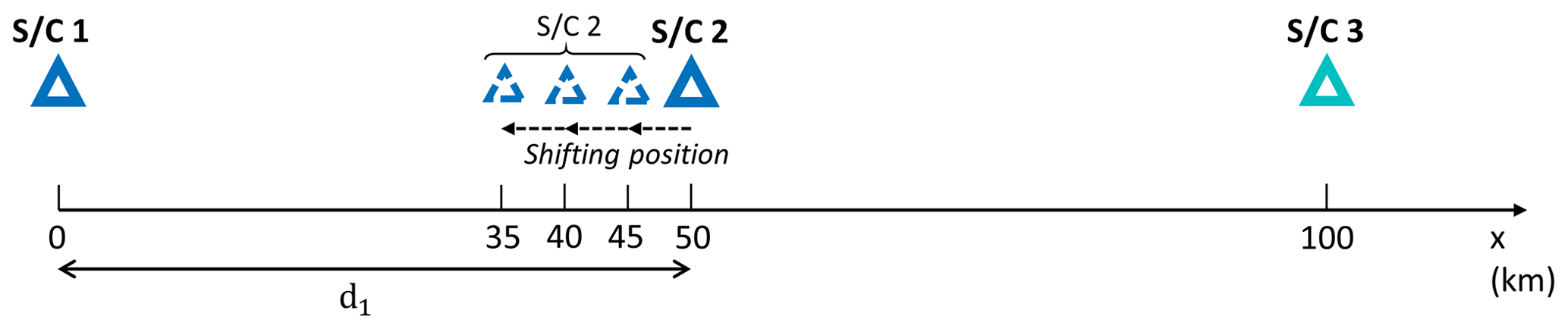
Figure 1 S/C configurations of both the two- and three-S/C test cases for the 1D analysis. The position of S/C 2 is shifted closer to S/C 1 for each analysis, thereby stepwise reducing their distance.

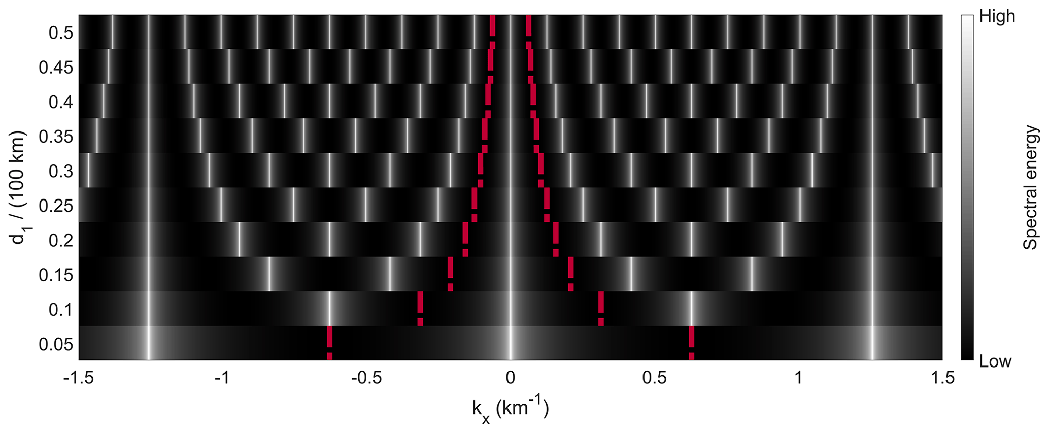
Figure 2 Wave-telescope-based spectral energy for different two-S/C configurations in a 1D configuration and regular spacing. The synthetic plane wave number used for modeling the artificial signal is $k={\mathrm{10}}^{-\mathrm{10}}$ km⁻¹. Each horizontal bar shows the 1D spectrum for the respective spacecraft distance given at the vertical axis. The red broken lines display the calculated spatial Nyquist limits.

An optimized zero adding – meaning the fewest zero-value sampling points added to obtain regular sampling – results if the new sampling times are defined by the greatest common divisor (gcd) of the original sampling distances ${\mathit{\tau }}_j=t_j-t_{\mathrm{1}}$. This becomes clear when considering a mathematical representation of the effective sampling distance (cf. Eyer and Bartholdi, 1999; Mignard, 2005):

$$\begin{array}{}\text{(21)}& t_j=t_{\mathrm{1}}+n_j{\mathit{\tau }}_{\mathrm{eff}}\end{array}$$

with n_j∈ℕ. For regular sampling, τ_eff equals the sampling time step, and n_j increases by 1 for each next sampling point. On the contrary, for irregular sampling, τ_eff has to be found with n_j being arbitrary. Zero adding will introduce sampling points for every missing n_j and thus transform the irregularly sampled time series into a regular one.

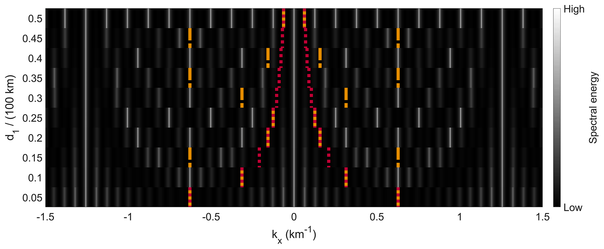
Figure 3 Spectral energy distribution of different three-S/C configurations in 1D and synthetic model wave number $k={\mathrm{10}}^{-\mathrm{10}}$ km⁻¹. Each horizontal bar shows the 1D spectrum for the respective spacecraft distance given at the vertical axis. The red dotted lines show the calculated spatial Nyquist limits without the third S/C (same as in Fig. 2), while the orange broken lines depict the spatial Nyquist limits calculated using the gcd.

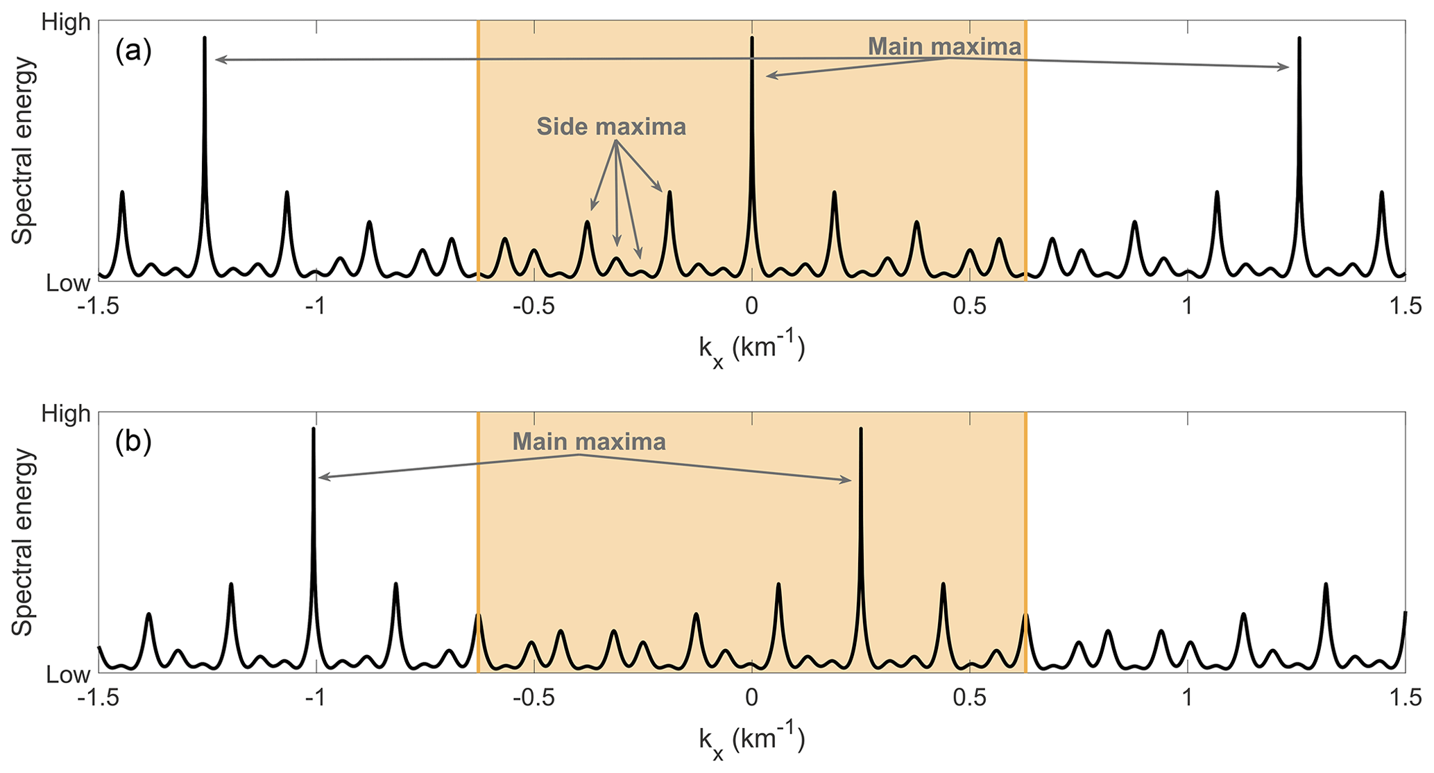
Figure 4 Spectral energy distribution of a three-S/C configuration with d₁ of 15 km (compare with Fig. 3). The spatial Nyquist limit is marked by the orange vertical lines, with the orange area in between marking the first Brillouin zone. In (a), an input wave vector of $k={\mathrm{10}}^{-\mathrm{10}}$ km⁻¹ has been used while in (b) the input wave vector is set to k=0.25 km⁻¹. As a result, the spectrum shifts to the right and is not symmetric around 0 anymore.

Equation (21) may be rewritten using only the sampling distances:

$$\begin{array}{}\text{(22)}& {\mathit{\tau }}_j=n_j{\mathit{\tau }}_{\mathrm{eff}}.\end{array}$$

Now, if we find the largest τ_eff possible fulfilling Eq. (22), this would be the largest divisor of all sampling distances τ_j. This represents the definition of the gcd (e.g., Bronshtein et al., 2007), and we can express the effective sampling distance by (cf. Mignard, 2005)

$$\begin{array}{}\text{(23)}& {\mathit{\tau }}_{\mathrm{eff}}=\gcd ({\mathit{\tau }}_{\mathrm{1}},\mathrm{\dots },{\mathit{\tau }}_n).\end{array}$$

Usually, the times or positions of the sampling points are not integer numbers but rational numbers: τ_j∈ℚ. An easy way to transform rational numbers into integer numbers is by multiplication with factor q=10 or q=100, depending on the accuracy of the values. A subsequent normalization is required, depending on the value of q. Thus, we may rewrite Eq. (23) to yield a generalized way for the determination of τ_eff:

$$\begin{array}{}\text{(24)}& {\mathit{\tau }}_{\mathrm{eff}}={\displaystyle \frac{\gcd (q\cdot {\mathit{\tau }}_{\mathrm{1}},\mathrm{\dots },q\cdot {\mathit{\tau }}_n)}{q}}.\end{array}$$

with q∈ℤ such that for all τ_j the product q⋅τ_j is an integer. With that, the gcd can essentially be computed for rational numbers. Therefore, the calculation of a largest common time step τ_eff for rational, irregular sampling times is straightforward. The determination of a Nyquist limit f_Neff, equivalent to the case of regular sampling, is possible.

The above approach can be adapted to other sampling spaces such as position space with sampling time differences τ_j becoming the aforementioned sampling position distances d_i and the largest common time step τ_eff becoming the largest common sampling position distance d_eff. We arrive at the 1D spatial Nyquist limit

$$\begin{array}{}\text{(25)}& k_{\mathrm{Ny}}={\displaystyle \frac{\mathit{\pi }}{d_{\mathrm{eff}}}},\end{array}$$

concurring with Eq. (14), the regular sampling case (in combination with Eq. 17). It is important to note that d_eff can be significantly smaller than the smallest sampling distance (the minimum of d_i); thus, k_Ny may become extraordinarily large.

Having defined both the spatial Nyquist limit for regularly (Eq. 14) and irregularly (Eq. 25) spaced sampling points, we use the wave telescope to visualize the differences of the spatial Nyquist limit for these two different cases. In 1D, we use two S/C (1 and 2; see Fig. 1) to show equally spaced sampling points and three S/C for irregular sampling. For each different model considered, the distance between S/C 1 and 2 is reduced from initially 50 km in steps of 5 km to a final 5 km. In the two-S/C case, this leads to an increasing spatial Nyquist limit. However, for the three-S/C case, when retaining the position of the third S/C at 100 km, irregularly spaced sampling points are created. The relation of the sampling distance and its corresponding spatial Nyquist limit is visualized in Figs. 2 and 3 for regular and irregular spacing, respectively.

For both the regular and irregular sampling case, we use the same synthetic plane wave with a wave number close to 0 km⁻¹, precisely 10⁻¹⁰ km⁻¹. This corresponds to a wavelength exceeding spacecraft distances by far. However, the wave telescope is still able to reproduce such a small wave number. It is chosen here solely for reasons of visualization as the results are symmetrically distributed around k=0 km⁻¹. This symmetry is displayed in more detail in Fig. 4a for one three-S/C irregular sampling case. As pointed out in Sect. 2.2, the wave telescope spectra are generally not symmetric around 0. Thus, a different, larger wave number results in a shift of the maxima in k space but does not change the periodicity itself as is shown in Fig. 4b, where the wave number was changed to k=0.25 km⁻¹. The absolute value of k is of minor interest as we are mainly interested in the numerical limitations of the method. In order to assure comparability, random noise added to the magnetic field data is only generated once and applied to each analysis.

The wave telescope energy spectra for all two-S/C configurations are shown in Fig. 2. The modeled wave with k≈0 km⁻¹ is clearly visible by its strong spectral peak at zero wave number. Additionally, periodic peaks due to aliasing are visible. The spatial Nyquist limit is calculated using Eqs. (14) and (17) and marked by the red lines. The agreement of this theoretically derived and calculated limit with the synthetic model case results is readily discernible as the repetition of maxima due to aliasing matches the spatial Nyquist limit.

By adding a third S/C at 100 km (irregularly spaced S/C case; see Fig. 3), the situation becomes more complex. Again, the wave telescope is able to successfully detect the original wave for all cases. In the case of regular spacing of the S/C, the case with d₁=50 km, we obtain the same result as for the two-S/C situation (cf. Fig. 2). However, the spatial Nyquist limit, now marked by the orange lines, depends on the gcd of both the distances d₁ and d₂. As a result, for some distances, the spatial Nyquist limit becomes much larger than for the corresponding two-S/C configuration (marked by the dotted red lines), while it is the same for others.

The periodicity for irregular sampling is more complex, with side maxima of different amplitudes appearing with different repeating patterns. This has also been observed by Bretthorst (2001) when using a discrete Fourier transform. These side maxima do not represent a true signal detection but are artifacts stemming from the different sampling distances. This makes the analysis of the spectrum difficult, as – without a priori knowledge of the input wave(s) – it is hard to determine which peaks represent true signal detections and which are mentioned artifacts (side maxima). In the following, we will refer to the true signal and its aliases as “main maxima”. The detailed representation of the spectrum of irregular sampling cases in Fig. 4 reveals the different amplitudes of the main and side maxima. Apart from the larger amplitude of the main maxima, there exists no apparent possibility to determine which peaks are true signal detections. Thus, the determination of the amplitude with satisfying accuracy is vital. Hence, a very large resolution is required due to the narrow width of the peaks (all visual presentations given here show a logarithmic energy spectrum). Especially for higher dimensions, high enough scan resolution of k space might become unachievable. In our analysis, the periodicity of the main maxima clearly matches the corresponding calculated Nyquist limit, showing the agreement of the theoretically calculated spatial Nyquist limit and the numerical analysis for the irregular sampling case as well. Therefore, the spatial Nyquist limit is a major aid in finding the main maxima, as within its limits (the orange area in Fig. 4) only one main maximum from every detected wave will be present.

3.2 The 2D case

The considerations of the impact of irregular spacing on the spatial Nyquist limit cannot simply be transferred from the 1D case to 2D and higher-dimensional situations. As orthogonality is not required for the reciprocal vectors, a separation of the two k vectors and projection onto one direction of the Cartesian coordinates does not provide a useful approach. This causes difficulties transferring the gcd approach from 1D to 2D situations.

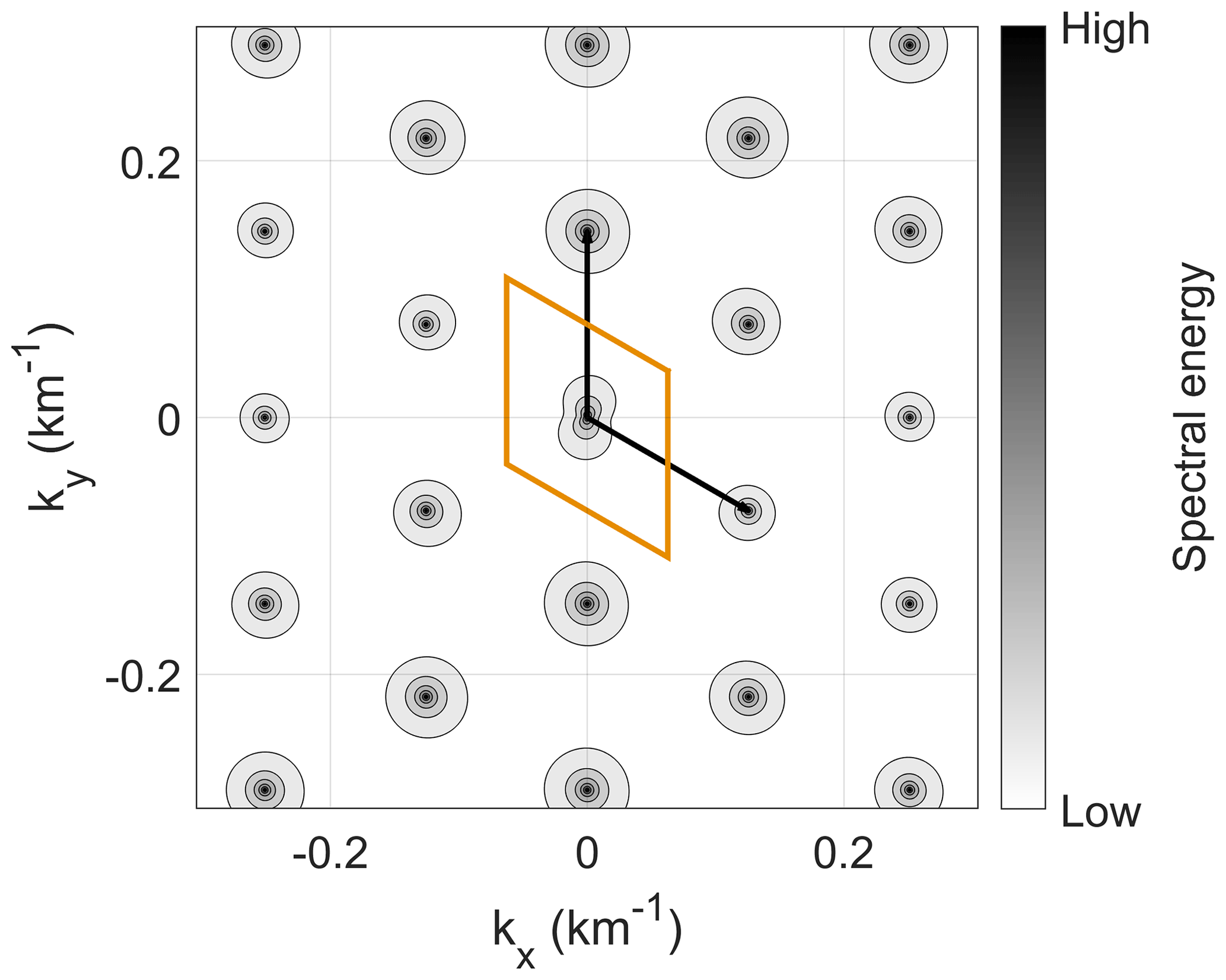
Figure 5 Spectral energy of the wave telescope analysis using three-S/C data with regular sampling in two dimensions. The spatial Nyquist limit periodic cell – calculated from the k vectors from Eq. (15) – is marked by the orange parallelogram.

In the 1D case, the spatial Nyquist limit can be determined by identifying the periodicity using the main maxima, disregarding lower-amplitude side maxima. Therefore, we also use this approach in 2D to determine the connection of the S/C configuration with the spatial Nyquist limit. In 2D, the regular sampling point case can be demonstrated with any configuration of spacecraft that lie on top of a 2D lattice. This is always the case for three S/C that do not form a line in space. More than three spacecraft form irregularly spaced sampling points. In this sense, regular does not refer to the configuration but rather the number of sampling points (spacecraft). We demonstrate a regular sampling point case with a configuration of three spacecraft forming an equilateral triangle. The resulting wave telescope power spectrum is shown in Fig. 5. Again a synthetic wave at the origin of k space represents the input signal. The spatial Nyquist limit periodic cell is now a parallelogram, spanned by the two k vectors determined from Eq. (15) and centered around the origin (cf. Narita et al., 2022). It clearly separates the true signal from the repetition of the maxima in both dimensions. Note that the logarithmic spectral energy is depicted to ensure the visibility of the maxima. In a linear presentation the spectral peaks are extremely sharp and easily overlooked.

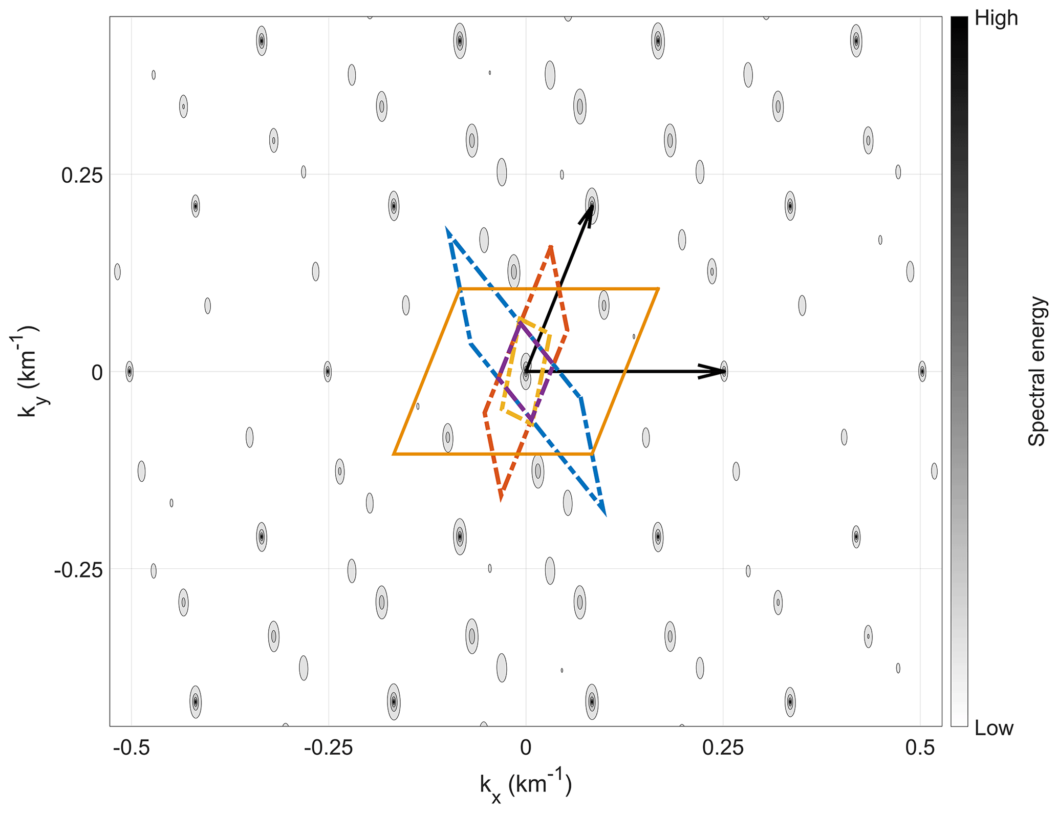
Figure 6 Spectral energy of a wave telescope analysis of four S/C in two dimensions. The spatial Nyquist limit periodic cells of subgroups of three S/C are marked by the dashed parallelograms in different colors. The larger orange solid-line parallelogram is the spatial Nyquist limit periodic cell derived by using the MLLL algorithm and testing for the shortest basis using enumeration. The black arrows indicate the basis vectors of the repetition of main maxima, determined from the model cases. The picture of k space shown here corresponds to the S/C locations in position space shown in Fig. 7.

The situation changes drastically when using irregular sampling for the same synthetic wave. The resulting spectrum for a 2D situation and four irregularly positioned S/C is presented in Fig. 6. Numerous local maxima are discernible with high-amplitude main maxima and lower-amplitude side maxima, as seen in the 1D case (cf. Fig. 4), but scattered in both dimensions. A 2D periodicity of the spectrum is visible. The main maxima – representing the input signal detection and its aliases – can be determined by only considering local maxima with an amplitude above a certain threshold value. With that, an overlaying superlattice structure becomes obvious with the two lattice vectors depicted by black arrows. These two vectors match the periodicity of the spectrum. Considering the k cells of each subgroup of three S/C, shown by the dashed line parallelograms, it is not obvious how the superlattice can be derived.

Based on modeling different irregular S/C configurations and determining their spectra, we can identify a suitable way to derive the superlattice. We only have the three translation vectors d_i but are searching for a 2D basis of the superlattice. By using every possible linear combination of the translation vectors in position space, a new (regular) lattice can be generated. The shortest two linearly independent vectors of that lattice are then used to calculate the reciprocal lattice via Eq. (15). This reciprocal lattice matches the visible periodicity in k space (respectively the two lattice vectors derived from the repetition of the main maxima). Thus, this is the superlattice we are looking for.

This new approach can be expressed mathematically by a set 𝒮 of vectors s formed by linear combination of the spacecraft translation vectors d_i:

$$\begin{array}{}\text{(26)}& \mathcal{S}=\mathit{\{}\mathit{s}=a_{\mathrm{1}}{\mathit{d}}_{\mathrm{1}}+a_{\mathrm{2}}{\mathit{d}}_{\mathrm{2}}+a_{\mathrm{3}}{\mathit{d}}_{\mathrm{3}}|a_i\in \mathbb{Z}\mathit{\}}.\end{array}$$

For an irregular spacecraft configuration, the number of translation vectors is always larger than the number of dimensions. From the set 𝒮, which fulfills 𝒮⊆ℚ², we seek a basis ${\mathit{s}}_{\mathrm{1}},{\mathit{s}}_{\mathrm{2}}\in \mathcal{S}$ constituting our superlattice basis vectors in position space. These have to be the shortest basis vectors, i.e., they have to fulfill the condition $\mathit{s}\in \mathcal{S}\backslash \mathit{\{}\mathrm{0},{\mathit{s}}_{\mathrm{1}},{\mathit{s}}_{\mathrm{2}}\mathit{\}}$:

$$\begin{array}{}\text{(27)}& \mathrm{0}<\left|{\mathit{s}}_{\mathrm{1}}\right|\le \left|{\mathit{s}}_{\mathrm{2}}\right|\le \left|\mathit{s}\right|.\end{array}$$

Additionally, they have to be linearly independent:

$$\begin{array}{}\text{(28)}& {\mathit{s}}_{\mathrm{1}}\ne c{\mathit{s}}_{\mathrm{2}}\end{array}$$

where $c\in \mathbb{R}\backslash \mathit{\left\{}\mathrm{0}\mathit{\right\}}$.

The above-described approach of k-space superlattice determination has one significant caveat. The number of possible lattice vectors created by linear combination is infinite. Therefore, one may give an upper boundary of the largest modulus of the linear combination multipliers $\left|a_i\right|$, thus confining scanning of the lattice vector space to a box. This box has to be sufficiently large to ensure that the sought basis vectors, s₁ and s₂, are among the determined lattice vectors. Depending on the decimal precision of the translation vectors, the required level of the upper boundary of $\left|a_i\right|$ can become prohibitively large and with it the box. Especially when expanding this method to higher dimensions, this box-bounded enumeration becomes computationally expensive inhibiting determination at some point. Thus, a more efficient method is needed.

The problem can be reformulated: in position space, we want to find the shortest possible basis of the superlattice formed by the vectors of the spacecraft distances (the translation vectors d_i). This means that one of the basis vectors found is the shortest possible lattice vector. Shortest refers to the moduli of the considered vectors.

The shortest vector problem (SVP) is a known fundamental problem in number theory, which is proven to be non-deterministic polynomial-time (NP) hard to solve (Ajtai, 1998). It can be approximated by finding a reduced basis using algorithms. Such is the Lenstra–Lenstra–Lovàsz (LLL) algorithm (Lenstra et al., 1982). This algorithm takes a matrix as input, constituted by the set of initial column lattice vectors (our translation vectors d_i). Following Hoffstein et al. (2008), the column vectors of the matrix are orthogonalized (but not normalized) via the Gram–Schmidt process. Afterwards, the length of the basis vectors is reduced by performing a special linear combination of the vectors under specific termination criteria. This iteration scheme finds a reduced basis, meaning that the shortest vector of the found basis g₁ is just

$$\begin{array}{}\text{(29)}& \left|{\mathit{g}}_{\mathrm{1}}\right|\le {\mathit{\beta }}^{\frac{m-\mathrm{1}}{\mathrm{2}}}\left|\mathit{l}\right|\end{array}$$

longer than the shortest non-zero vector l of the set of all lattice vectors. The parameter β can be chosen out of the interval [0.25,1) in a trade-off of shortness of the reduced basis and algorithm termination speed. The number of dimensions m is equal to the length of the considered vectors (Bremner, 2011, p. 60). A detailed description of the LLL algorithm is out of the scope of the present study. For further discussions, the reader is referred to Hoffstein et al. (2008) and Bremner (2011).

However, the LLL algorithm only works for linearly independent lattice vectors. As our initial set of translation vectors constituting the lattice is a linearly dependent set (see Eq. 26), a modified version of LLL has to be used, namely, MLLL (Pohst, 1987), which essentially applies LLL to an expanded dimensional space. The LLL algorithm is known to “usually” provide the shortest vector for low dimensions (Odlyzko, 1989). However, for our purposes, we have to be sure that the shortest possible basis is found and thus the shortest vector is indeed part of the calculated basis. This can only be assured by using basis enumeration algorithms, which use the reduced basis of LLL (respectively MLLL) as an input. These algorithms determine the shortest basis (here consisting of the two shortest vectors) by scanning every possible vector within a confined vector space and thus finding the set of vectors fulfilling the auxiliary conditions (27) and (28). For the simple cases considered here, the abovementioned box-bounded enumeration is sufficient. Alternatively, enumeration algorithms like the Fincke–Pohst (Fincke and Pohst, 1985) algorithm may be used. It is much more efficient than standard enumeration algorithms (Bremner, 2011, pp. 155), among them the box method. For details about the different algorithms, the reader is referred to the cited literature.

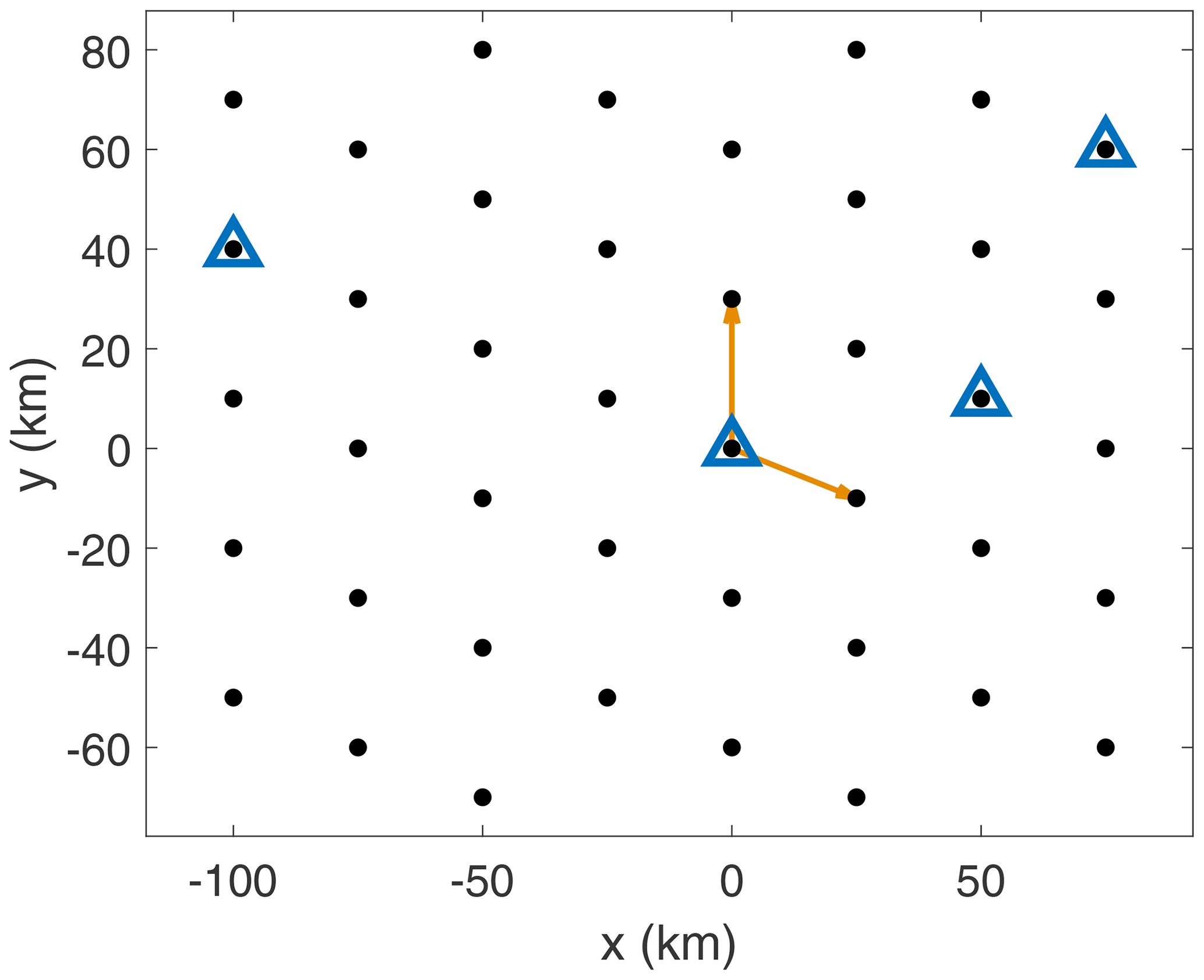
Here, we perform MLLL on an integer basis, using the code (respectively the website) of Matthews (2011). The integer basis is acquired by shifting the decimal point on the translation vectors. Then, box-bounded enumeration is performed to assure that the found basis is indeed the shortest one. Additionally, checks using the Fincke–Pohst algorithm were carried out. For all simulated S/C configurations assessed in this work, both in 2D and 3D, MLLL already provided the shortest basis. The S/C configuration corresponding to Fig. 6 with the position-space superlattice computed from linear combination along with MLLL-determined lattice vectors is presented in Fig. 7. Clearly, the lattice vectors fit the superlattice and the S/C configuration.

To summarize, by calculating the shortest basis from the original S/C positions and afterwards converting the acquired basis vectors to reciprocal space, the spatial Nyquist limit in 2D can be determined. The above-shown synthetic data analysis has been carried out for different S/C configurations, at all times confirming the observed behavior.

Figure 7 S/C positions in position space (blue triangles) corresponding to Fig. 6 along with the superlattice (the black dots) generated by linear combination of the S/C translation vectors. The MLLL-determined shortest basis fitting to that superlattice is shown by the orange arrows.

3.3 The 3D case and generalization

Before applying our findings in 2D to the 3D wave telescope, we need to generalize the calculation of a position-space superlattice to arbitrary dimensions. Firstly, it can be shown that the application of the MLLL algorithm in 1D is equivalent to the gcd formulation (Bremner, 2011, p. 107). Additionally, one may also show that linear combination in 1D is synonymous to the gcd formulation. This shows that the 2D approach works in 1D as well. Thus, heuristically, the combination of MLLL and lattice enumeration algorithms in 2D, substituting expensive linear combination, can be seen as the extension of the gcd to higher dimensions. Hence, in mathematical terms, Eq. (26) may be generalized for an arbitrary number of dimensions m (here, heuristically even m>3 is possible) and S/C n using n−1 (column) translation vectors ${\mathit{d}}_{\mathrm{1}},\mathrm{\dots },{\mathit{d}}_{n-\mathrm{1}}$ by

$$\begin{array}{}\text{(30)}& \mathbf{DA}=\mathbf{S}\end{array}$$

with

$$\begin{array}{}\text{(31)}& {\displaystyle }\mathbf{D}=\left(\begin{array}{ccc}{\mathit{d}}_{\mathrm{1}}& \mathrm{\cdots }& {\mathit{d}}_{\mathrm{n}-\mathrm{1}}\end{array}\right)=\left(\begin{array}{ccc}{\mathit{d}}_{\mathrm{1},\mathrm{1}}& \mathrm{\cdots }& {\mathit{d}}_{n-\mathrm{1},\mathrm{1}}\\ \mathrm{⋮}& \mathrm{\ddots }& \mathrm{⋮}\\ {\mathit{d}}_{\mathrm{1},m}& \mathrm{\cdots }& {\mathit{d}}_{n-\mathrm{1},m}\end{array}\right),\text{(32)}& {\displaystyle }\mathbf{A}=\left(\begin{array}{ccc}{a}_{\mathrm{1},\mathrm{1}}& \mathrm{\cdots }& a_{m,\mathrm{1}}\\ \mathrm{⋮}& \mathrm{\ddots }& \mathrm{⋮}\\ a_{\mathrm{1},n-\mathrm{1}}& \mathrm{\cdots }& a_{m,n-\mathrm{1}}\end{array}\right),\text{(33)}& {\displaystyle }\mathbf{S}=\left(\begin{array}{ccc}{\mathit{s}}_{\mathrm{1}}& \mathrm{\cdots }& {\mathit{s}}_m\end{array}\right)=\left(\begin{array}{ccc}{\mathit{s}}_{\mathrm{1},\mathrm{1}}& \mathrm{\cdots }& {\mathit{s}}_{m,\mathrm{1}}\\ \mathrm{⋮}& \mathrm{\ddots }& \mathrm{⋮}\\ {\mathit{s}}_{\mathrm{1},m}& \mathrm{\cdots }& {\mathit{s}}_{m,m}\end{array}\right),\end{array}$$

where $\mathbf{D}\in {\mathbb{Q}}^{m\times (n-\mathrm{1})}$, $\mathbf{A}\in {\mathbb{Z}}^{(n-\mathrm{1})\times m}$ and $\mathbf{S}\in {\mathbb{Q}}^{m\times m}$. In order for the column vectors ${\mathit{s}}_{\mathrm{1}},\mathrm{\dots },{\mathit{s}}_m$ to represent the shortest basis, the coefficients of the matrix A have to be chosen in such a way that the basis vectors s_i are the shortest possible m linearly independent vectors. Having two unknowns in Eq. (30), one has to turn to a basis reduction algorithm combined with an enumeration algorithm to determine the basis vectors s_i, as explained for the 2D case. Here, we use MLLL to calculate a reduced basis and subsequent box-bounded enumeration to ensure the MLLL basis is indeed the shortest basis. Having the shortest possible basis in position space, using the known formulae, this basis may be transferred to k space to find the sought periodic cell (respectively the spatial Nyquist limit).

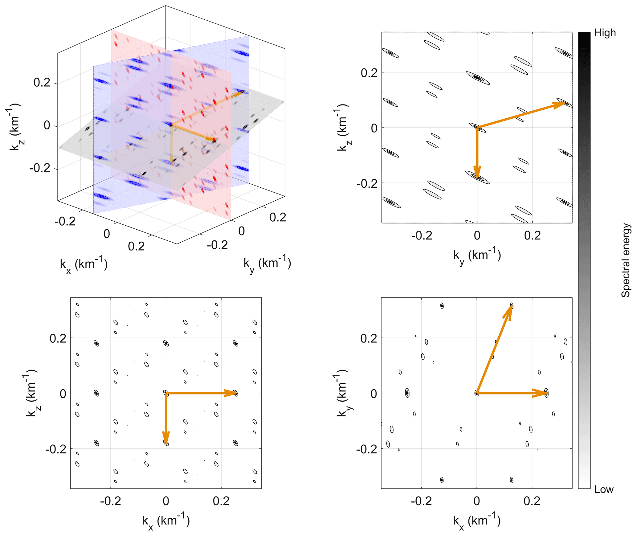
Figure 8 Slices of a wave telescope energy spectrum in 3D along the planes spanned by the MLLL-calculated k vectors (orange arrows). A five-S/C configuration is used in this case. The 2D plots show the projection of the three slices onto two of the three Cartesian coordinates.

We shall test whether such a calculated basis in 3D fits the synthetic data analysis of 3D wave telescope results. As for the 2D case, this is tested with several different S/C configurations. Here, the irregular case is presented for five S/C or more. Again, with an input wave close to 0 km⁻¹, the energy spectrum in k space is computed. A closer look into a 3D visualization shows that k space periodicity converges with the MLLL-derived k vectors.

Slices from such a 3D picture along the planes spanned by the three computed k vectors (orange arrows) are shown in Fig. 8 for a case of five S/C with the positions

$$\begin{array}{}\text{(34)}& \mathit{r}=\left(\begin{array}{ccccc}\mathrm{0}& \mathrm{50}& \mathrm{75}& -\mathrm{100}& -\mathrm{125}\\ \mathrm{0}& \mathrm{10}& \mathrm{60}& \mathrm{40}& \mathrm{40}\\ \mathrm{0}& \mathrm{35}& \mathrm{175}& \mathrm{0}& \mathrm{35}\end{array}\right)\mathrm{km},\end{array}$$

where the column vectors are S/C position vectors. The MLLL-reduced lattice (also being the shortest basis) then is

$$\begin{array}{}\text{(35)}& \mathbf{S}=\left(\begin{array}{ccc}\mathrm{0}& \mathrm{25}& \mathrm{0}\\ \mathrm{20}& -\mathrm{10}& \mathrm{10}\\ \mathrm{0}& \mathrm{0}& -\mathrm{35}\end{array}\right)\mathrm{km},\end{array}$$

where the column vectors depict the three linearly independent lattice base vectors.

In such way we tested different S/C configurations with up to 10 S/C. Within error of resolution, in all cases, the k vectors determined from the MLLL-reduced superlattice concur with the repetition of main maxima in k space. Already for 3D and S/C numbers as high as 10, computation time is a constraint in the wave telescope calculations, and the limited number of data points is a problem for visual analysis. In conclusion, the analysis of the different model cases strongly supports our heuristically based generalization to higher dimensions.

4 Application and data analysis

The above-presented mathematical formulae, heuristic derivations and numerical analyses show how the S/C positions, acting as irregularly spaced spatial sampling points, can be used to derive the spatial Nyquist limit without any knowledge about the considered physical quantity, i.e., here the magnetic field. However, regarding the synthetic data model cases, only simple cases were analyzed due to computational and thus resolution limits. In reality, position errors of the S/C will enormously alter the calculated spatial Nyquist limit because of its reciprocal nature. Very small errors can lead to a near-infinite spatial Nyquist limit, which is not resembling realistic capabilities of, for example, the wave telescope analysis. Especially for the wave telescope, due to time averaging of the position combined with the spacecraft's relative position variations due to orbital mechanics, it is vital to incorporate the position errors into the lattice calculations.

In the following, a summarized approach to determine the spatial Nyquist limit (for arbitrary m and n) is given. First, to account for the aforementioned S/C position errors, the accuracies in the S/C positions in the calculations should be reduced to nearest larger orders of magnitude of the respective uncertainty. After that, a reduced linearly independent basis in position space should be determined by using the MLLL algorithm. To ensure this MLLL-reduced basis is the shortest possible basis, one should employ a basis enumeration algorithm on the reduced basis. The found shortest basis in position space can be used to determine the reciprocal vectors in k space by applying the appropriate formulae (Eqs. 14, 15 and 16, depending on the number of dimensions m). Then, the spatial Nyquist limit may be calculated with Eq. (17), constituting the periodic cell both in positive and negative directions. However, to determine the unit cell of the superlattice in k space within which no aliasing will be present, the Wigner–Seitz cell has to be constructed from the double-length spatial Nyquist vectors. This unit cell represents the first Brillouin zone, and analysis of k space should focus only on this region.

Additionally, in order to determine the actual wave vector(s) of the signal, either a very high scan resolution to ensure resolution of the highest maximum or a method to dampen the side maxima is needed. The side maxima emerge due to the spatial Nyquist limits of the regular-sampling-point subsets of the original irregular sampling points. Similar observations have been remarked by Bretthorst (2001). We show this behavior here with the wave telescope in 2D for the case shown in Figs. 6 and 7. The four irregularly spaced S/C yield four regularly spaced subsets of three S/C each. The wave telescope analysis of these four subsets is shown in Fig. 9. As there is only regular spacing of the sampling points (respectively S/C), only the known periodicity can be observed – all discernible maxima are main maxima, meaning the true maximum and its aliases. Due to different S/C used in each of the subsets, the parallelepiped (marked in each plot) is different each time. However, marked by the arrows, the spatial Nyquist limit k vectors of the combined, irregular four-S/C configuration converge with a common maximum to all four subsets.

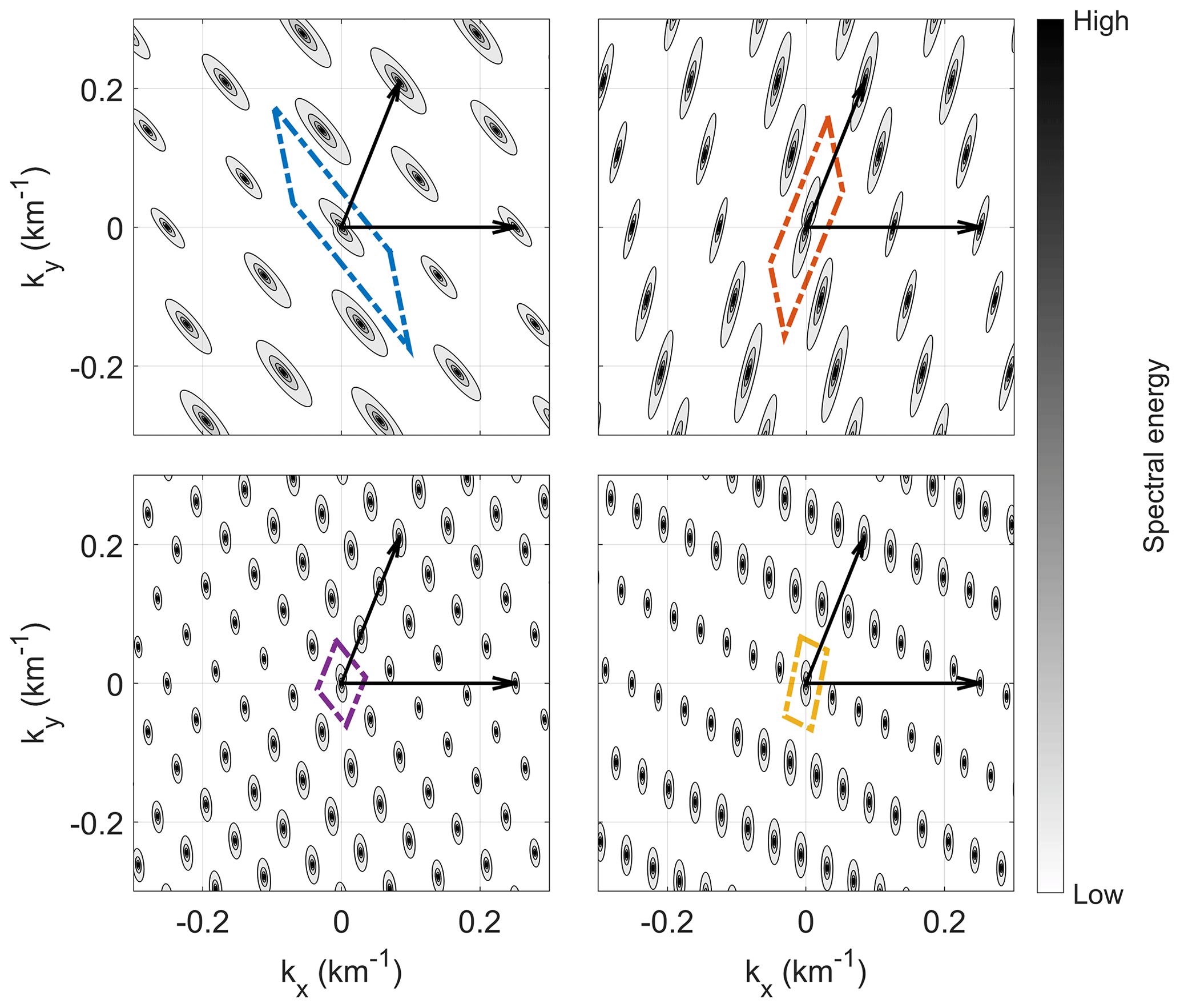
Figure 9 Spectral energy of wave telescope analysis of subsets of the four-S/C configuration from Fig. 7. The spatial Nyquist limit periodic cell of each subset of three S/C is marked by the dashed parallelograms in different colors.

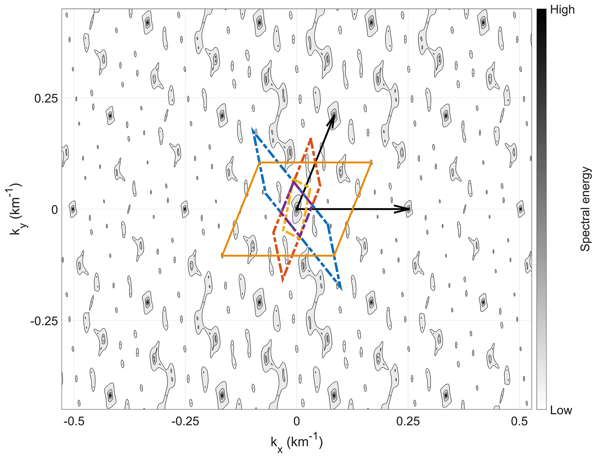
Figure 10 Spectral energy of the combination (element-wise multiplication) of the subsets of the four-S/C configuration of Fig. 7 in 2D. The spatial Nyquist limit periodic cells of subgroups of three S/C are marked by the dashed parallelograms in different colors. The larger orange solid-line rectangle is the spatial Nyquist limit periodic cell derived by using the MLLL algorithm and testing for the shortest vector using enumeration. The black arrows indicate the base vectors of the repetition of main maxima, determined from the model cases. This spectrum is similar to the original four-S/C spectrum shown in Fig. 6.

By combining spectra of the subsets, e.g., by element-wise multiplication and appropriate normalization, a spectrum quite close to the actual four-S/C spectrum can be obtained (see Fig. 10). Thus, the following rule of thumb can be applied to identify the main maxima: determine the spectrum for all regularly spaced subsets of sampling points and only focus on the region around the maxima that is common to all these subsets. All other maxima may be damped by appropriate filtering. A regular spaced subset of sampling points is constituted by a subset of m+1 sampling points that span the m spatial dimensions.

5 Summary and Conclusions

In this study, we have derived an analytical representation of the spatial Nyquist limit, the aliasing limit in multi-dimensional k space, for irregularly spaced sampling points. This has been verified using the wave telescope technique – generalized to arbitrary dimensions – applied to synthetic plane wave data sampled at irregularly distributed S/C configurations in different dimensions m, where the number of S/C (the spatial sampling points) is larger than m+1. By this modeling, first it has been shown that for non-uniform sampling in 1D also the wave telescope technique shows the same aliasing features as in time or frequency, e.g., the ordinary DFT (Bretthorst, 2001) and the Lomb–Scargle periodogram (VanderPlas, 2018). We have extended this to 2D and 3D with configurations of more than 4 and up to 10 S/C. The computed wave telescope energy spectra show spectral structures, like main and side maxima, that repeat themselves in periodic cells in k space because of aliasing. Using the periodicity of the main maxima – which resemble input signal detections and their aliases – the spatial Nyquist limit has been determined. In all cases, within limits of the resolution, it was possible to concurrently derive the same overlaying periodicity and thus spatial Nyquist limit from the determination of the shortest possible basis of the position-space spacecraft translation vectors, using the MLLL lattice reduction algorithm verified by lattice enumeration. This allows for the analytical determination of the spatial Nyquist limit of multi-spacecraft measurements for the wave telescope without any need to look at spectra periodicity and more precisely without any a priori knowledge of the measured data. Only the positions of the S/C (respectively of the sampling points) are required to determine the spatial Nyquist limit. Thus, the above-presented algorithm serves as a key element for planning the spatial distribution of future multi-point spacecraft missions. In summary, we give a model-based verification of the heuristically derived generalization of the spatial Nyquist limit for irregularly spaced sampling points (respectively S/C) to arbitrary numbers of dimensions and sampling points.

The aforementioned side maxima in the wave telescope spectra are shown to be artifacts of regular subsets of sampling points. Their damping – along with sensible treatment of S/C position errors in the calculation of the spatial Nyquist limit – can help one to yield wave telescope spectra with reduced to vanished aliasing. Only by including these considerations does the analysis of magnetic field data with the wave telescope of multi-point multi-scale missions like HelioSwarm (nine S/C) become manageable from an aliasing point of view. In combination with a statistical error quantification of the wave telescope technique in Broeren and Klein (2023), it is possible to precisely quantify the wave telescope's capabilities when using configurations of more than four S/C.

As the wave telescope acts as a power spectrum estimator substituting spatial Fourier transform PSD estimation in multiple dimensions, the results from this study, precisely the analytical representation of the spatial Nyquist limit, can be directly transferred to different fields of research that are using multi-dimensional Fourier analysis to estimate power spectra or other spectrum estimators with irregular sampling points. Such fields are mathematics, nuclear magnetic resonance (NMR) analysis or general signal processing. Also, the generalized wave telescope is not only restricted to geophysics but also applicable to wave and spectrum determination in even-higher-dimensional data. For example, the wave telescope can be applied to higher-dimensional phase space, e.g., by combining magnetic field and density data to a four-dimensional dataset. This allows for comprehensive and simultaneous data analysis without the need for later correlation analysis of different physical quantities.