Parallel electric fields produced by ionospheric injection

It is well known that there exists a thin layer in the lower boundary of the ionosphere between altitudes of 80 and 140 km in which collisional ions and collisionless electrons mix. Local breakdown of charge neutrality may be initiated in this layer by electric fields from the magnetosphere as well as by electric fields generated there by the local neutral winds. The breakdown may be momentarily canceled by Pedersen currents, but complete neutralization is prevented because some ionospheric plasmas are released as outflows by parallel electric fields. Those parallel electric fields are produced by inherent plasma processes in the polar ionosphere and act as auroral drivers. A new scenario creating parallel potential gradients is proposed.

1 Introduction

The Poynting flux of fields and the particle momentum carried by a double layer or an electrostatic shock generate parallel electric fields in the magnetosphere (Block, 1977; Goertz and Boswell, 1979). Field-aligned plasma flows in converging field geometry are mechanical energies that excite parallel electric fields by the charge separations along the field lines due to the magnetic mirroring of electrons and ions (Sato, 1982; Schriver and Ashour-Abdalla, 1993). Open fields interacting with the solar wind and a charge separation across the nightside magnetosphere due to the plasma convections in the magnetosphere create parallel electric fields (Lyons, 1980; Stern, 1981). These parallel potentials associated with the magnetospheric generators are used to infer FAC (field-aligned current) in the magnetosphere (Knight, 1973; Chiu and Schulz, 1978).

The ionosphere as a generator has the capability to produce electrostatic potential itself once the electric fields are transmitted along field lines into the auroral zone from the magnetosphere or are produced there by the local neutral winds (Saka, 2021b). While those electric fields that have penetrated the E region may accumulate collisionless electrons at a leading edge of flow channels caused by the E×B drift, collisional ions cannot follow them. The negative potential thus produced at the leading edge of flow channels in the E region generates upward electric fields as an auroral driver. Although this conjunction is inconsistent with Gauss's theorem, it can be understood if a positive space charge was generated immediately above the ionosphere. The above description is consistent with the formation of an incomplete Cowling channel (Baumjohann, 1980), except that upward field-aligned currents are created at the negatively charged southern border (Saka, 2021b).

Ionospheric potential may be observed in the global current circuit of the ionosphere–atmosphere–earth system. The currents in this circuit are generated in the atmosphere by charge separation processes in tropical convective storms. The current influenced by the ionospheric potential can be detected in this global circuit by monitoring the vertical component (B_z) of the ground magnetometer data. Reduction of B_z on the ground correlates with a decrease in the atmospheric electric field on the ground (Minamoto and Kadokura, 2011). Such a correlation would occur in connection with the potential drop in the ionosphere above the ground station (Saka, 2021a).

The proposed new scenario referred to as ionospheric injection is summarized in Sect. 2. A summary and discussion are presented in Sect. 3.

2 Ionospheric injection

The distribution of the pitch angle along the field lines can be expressed using a constant of the motion:

$$\begin{array}{}\text{(1)}& \mathit{\mu }={\displaystyle \frac{m_q}{\mathrm{2}B}}{v}^{\mathrm{2}}{\sin }^{\mathrm{2}}\mathit{\alpha }.\end{array}$$

Here, α denotes the pitch angle at the magnetic field B, and $m_q{v}^{\mathrm{2}}/\mathrm{2}$ is the kinetic energy of particle q. Substituting B_R at the mirror height (sin ²α=1), altitude profiles of the pitch angle in the absence of the parallel electric fields can be given as

$$\begin{array}{}\text{(2)}& {\sin }^{\mathrm{2}}\mathit{\alpha }={\displaystyle \frac{B}{B_{\text{R}}}}.\end{array}$$

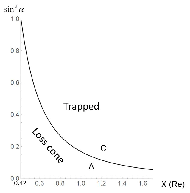
Figure 1 Altitude profiles of ${\sin }^{\mathrm{2}}\mathit{\alpha }=B/B_{\text{R}}$ in the dipole geometry of L=6. X (Re) denotes equatorial projection of the altitudes from the ionosphere (X=0.42 Re) to 10 520 km above it (X=1.70 Re). B_R represents field magnitudes at the ionosphere. Trapped particles filled area C. Loss cone particles filled area A. This curve can be given in the absence of the parallel electric fields.

Figure 1 shows an altitude profile of sin ²α along L=6 of the dipole fields from the ionosphere (100 km) to 10 520 km above it.

The pitch-angle curve along the field lines shown in Fig. 1 could be modified by the presence of the parallel electric fields. Two types of parallel electric fields are discussed, one being transient and the other steady-state. The direction of the transient electric field is downward into the ionosphere, and that of the steady-state electric field is upward out of the ionosphere (Fig. 2).

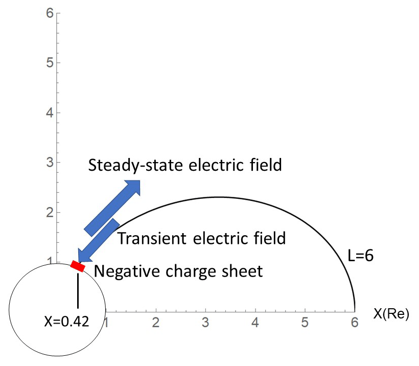
Figure 2 Transient electric fields are produced by the negative charge sheet shown in red. A negative charge sheet is shown in red at the polar-ionosphere-produced transient electric fields. A steady-state electric field was initiated by the transient electric field via Persson's theorem (see text). Transient electric fields are shielded by the space charge deposited in association with the onset of steady-state electric fields.

2.1 Excitation of transient electric fields

We assume that negative potential regions are produced by the local breakdown of the charge neutrality. This breakdown occurred in a thin layer located at boundaries between the mesosphere and thermosphere where collisional ions and collisionless electrons mix (Rishbeth and Garriot, 1969). The thin layer extends between altitudes of 80 and 140 km and is hereafter referred to as the ionosphere.

We assume that the negative charge sheet (1280 km in longitude and 128 km in latitude) was developed in the ionosphere. The thickness of the sheet is assumed to be equivalent to the same 60 km thickness of the ionosphere. The emerging charge density is assumed to be 5×10² m⁻³ in the sheet. Vertical electric fields generated by the negative charge sheet are directed down into the ionosphere (Fig. 2). Altitude profiles of the downward electric fields through the center of the sheet are colored in red in Fig. 3a. For comparison, the magnetic mirror force (mV m⁻¹) is presented in black, assuming μ=0.16 eV nT⁻¹, corresponding to $\frac{{\text{mV}}_{\perp }^{\mathrm{2}}}{\mathrm{2}}=\mathrm{1}$ keV at X=1 Re (6240 nT). The force arising from electrostatic fields exceeds the magnetic mirror force below 3643 km in altitude. When the spatial scale of the negative charge sheet decreased to 640 km × 64 km, the crossover altitudes of the two forces decreased to 1830 km (Fig. 4a).

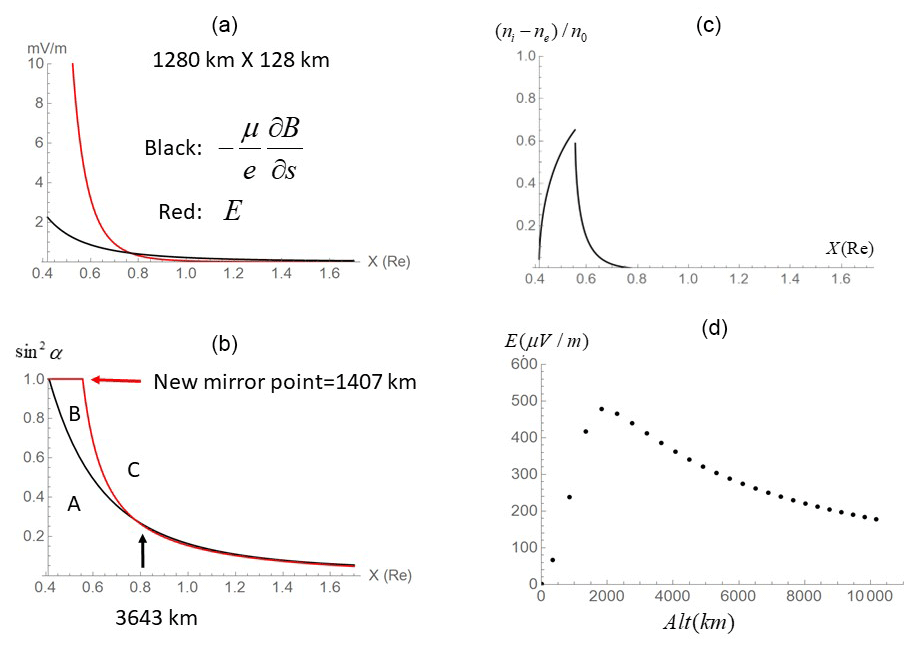
Figure 3 Negative charge sheets extending 1280 km in longitude and 128 km in latitude are generated in the polar ionosphere. (a) Equatorial projection of altitude profiles of the magnetic mirror force (black) and the vertical electric fields (red): X (Re) denotes the equatorial projection of the altitudes from the ionosphere (X=0.42 Re) to 10 520 km above it (X=1.70 Re). It is assumed that μ=0.16 eV nT⁻¹. Vertical electric fields exceed the magnetic mirror force below 3643 km. Note that amplitudes are presented in millivolt per meter. (b) Pitch-angle curve, ${\sin }^{\mathrm{2}}\mathit{\alpha }=B/B_{\text{R}}$, for electrons in the absence of the parallel electric fields (black) and those modified by the vertical electric fields (red): electrons when affected by the vertical electric fields moved their mirror point to higher altitudes at 1407 km above the ionosphere. There are three regions in pitch-angle profiles, i.e., A, B, and C (see the text). (c) Difference in number density n_i−n_e normalized by n₀: number densities of ions (n_i) and electrons (n_e) are calculated by integrating a Maxwellian distribution over velocity space. Plasma density in the loss cone is empty (see text). The plot along L=6 started from the ionosphere (X=0.42 Re) to 10 520 km above it (X=1.70 Re). Real density is given by multiplying n₀. The density gap at X=0.54 Re is caused by a discontinuous change in sin ²α. (d) Altitude profiles of steady-state electric fields $E_{//}$ (upward, µV m⁻¹) along field lines: the horizontal axis shows altitudes in kilometers of the field lines along L=6. Note that the ionosphere is at 0 km.

Downward electric fields change the pitch-angle trajectories of electrons approaching the ionosphere from the magnetosphere by decelerating the parallel velocities. The mirror height moved to 1407 km (Fig. 3b). For the smaller-scale charge sheet, the new mirror height is 590 km (Fig. 4b). For purposes of reference, pitch-angle trajectories in the absence of the parallel electric fields (sin ²α vs. X) are plotted in black. Pitch-angle trajectories of electrons bend clockwise with the new mirror height. These are shown in Figs. 3b and 4b in red. Ions may not change pitch-angle trajectories in a bounce time of electrons (a few seconds) because of the mass ratio.

As a result, there appeared three regions designated as A, B, and C in the pitch-angle plane (Figs. 3b and 4b). In A, electrons and ions are in a loss cone; in B, ions are trapped but electrons from the loss cone decelerated by downward electric fields filled this region due to magnetic mirroring; and in C, electrons and ions are trapped. Pitch-angle discrepancy appears only in region B: electrons are loss cone populations, while ions are trapped populations.

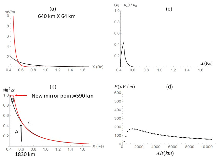
Figure 4 Same as Fig. 3 but for a half-sized negative charge sheet (640 km in longitude and 64 km in latitude).

According to Persson (1963), the number densities of hot plasmas are calculated by substituting an isotropic Maxwellian distribution of temperature T_q,

$$f_{\text{trap}}(v_{//},v_{\perp })={\left({\displaystyle \frac{m_q}{\mathrm{2}\mathit{\pi }k{T}_q}}\right)}^{\mathrm{3}/\mathrm{2}}\exp \left(-{\displaystyle \frac{m_q}{\mathrm{2}k{T}_q}}\left(v_{//}^{\mathrm{2}}+v_{\perp }^{\mathrm{2}}\right)\right),$$

out of the loss cone and $f_{\text{loss}}(v_{//},v_{\perp })=c{f}_{\text{trap}}(v_{//},v_{\perp })$ in the loss cone into

$$\begin{array}{}\text{(3)}& {\displaystyle \frac{n_q}{n_{\mathrm{0}}}}=\mathrm{2}\mathit{\pi }\int \left[f_{\text{trap}}(v_{//},v_{\perp })+f_{\text{loss}}(v_{//},v_{\perp })\right]v_{\perp }\mathrm{d}{v}_{\perp }\mathrm{d}{v}_{//}.\end{array}$$

Here, q is applicable to either electrons or ions. We assume that loss cone particles are removed from the flux tubes and are empty (c=0) prior to the auroral evolutions arising out of the onset arc or before the following auroral onset.

The normalized density difference, $(n_i-n_e)/n_{\mathrm{0}}$, before the auroral onset (c=0) is shown in Fig. 3c (Fig. 4c). When we chose c=0.5, the normalized density difference shown in Fig. 3c (Fig. 4c) was reduced by half. Positive charges emerged immediately above the ionosphere. The excess electrons repelled from both hemispheres due to magnetic mirroring would create the electron-rich regions in the magnetosphere.

2.2 Steady-state solution of parallel electric fields

In the one-dimensional model, parallel electric fields at s₁ are calculated by integrating the density difference along field lines s:

$$\begin{array}{}\text{(4)}& E_{//}\left(s_{\mathrm{1}}\right)=\underset{s_{\mathrm{0}}}{\overset{s_{\mathrm{1}}}{\int }}{\displaystyle \frac{e(n_{\text{i}}-n_{\text{e}})}{{\mathit{\epsilon }}_{\mathrm{0}}}}\mathrm{d}s.\end{array}$$

Here, s₀ denotes the ionospheric altitude where integration starts.

These are plotted in Fig. 3d (Fig. 4d), starting from the ionosphere (0 km) to a point at 10 520 km. At this altitude, the upward electric fields have not vanished because an electron-rich region may be located far up in the magnetosphere. To plot profiles of the parallel electric fields, a geometrical factor ($\sqrt{B_{s_{\mathrm{1}}}/B_{s_{\mathrm{0}}}})$ was multiplied by $E_{//}\left(s_{\mathrm{1}}\right)$ to adjust the diverging geometry of the dipole configuration. $E_{//}\left(s_{\mathrm{1}}\right)$ is linearly proportional to the background hot plasma density supplied from the tail. In this plot, a hot plasma density $n_{\mathrm{0}}={\mathrm{10}}^{-\mathrm{1}}$ m⁻³ was assumed.

These parallel electric fields are generated by charge separations along the diverging magnetic fields, with positive charges immediately above the ionosphere and negative charges in the magnetosphere constituting steady-state solutions of the flux tubes (Alfven and Falthammar, 1963; Persson, 1966). Generation of upward electric fields above the negative charge sheet resembles a battery connected in series to the negative electrode in the ionosphere. Transient electric fields of opposite polarity would be shielded by the space charge built up along the field line. The lifetime of the transient electric fields is a few seconds, a time required for building up the space charge or bounce time of electrons. Steady-state electric fields may persist until charge separation along field lines is neutralized. Because the flux tube contains parallel electric fields pointing upward, neutralization may occur locally and intermittently when accompanying auroral precipitation. We assume that the loss cone electrons are removed by the downward acceleration before the start of the following auroral evolutions.

3 Summary and discussion

Vertical electric fields develop transiently in the ionosphere and produce different angular distributions of ions and electrons in the magnetosphere. These transients yield charge separations along the field lines. Charge separations along the field lines produce steady-state parallel electric fields in the magnetosphere.

The transients are usually triggered by the transverse electric fields transmitted from the magnetosphere during the dipolarization onset. We also consider cases where breakdown of the charge neutrality was initiated in the polar ionosphere by neutral winds. Neutral wind generates a positive charge on the leading edge of the wind channel and a negative charge on the trailing edge; the E×B drift (E is polarization electric fields in the wind channel) generates a negative charge to the one side and a positive charge to the other side of the wind channel. Auroras are produced in the negative charge region. If the wind velocity is weaker than the E×B drift, breakdown of the charge neutrality may not happen because polarization drift of ions suppresses the charging up of the ionosphere. Wind velocities on the order of 10³ m s⁻¹ are necessary to produce substorm auroras by the neutral wind. This scenario may be reminiscent of auroras among gas planets in the solar system such as weather-driven auroras on Saturn (Chowdhury et al., 2021).