Analysis of in situ measurements of electron, ion and neutral temperatures in the lower thermosphere–ionosphere

Simultaneous knowledge of the temperatures of electrons, ions and neutrals is key to the understanding and quantification of energy transfer processes in planetary atmospheres. However, whereas electron and ion temperature measurements are routinely obtained from ground-based incoherent scatter radars, simultaneous measurements of electron, ion and neutral temperature measurements can only be made in situ. For the Earth's lower thermosphere–ionosphere, the only available comprehensive in situ dataset of electron, ion and neutral temperatures to date is that of the Atmosphere Explorers C, D and E and the Dynamics Explorer 2 missions. In this study we first perform a cross-comparison of all co-temporal and co-spatial measurements between in situ electron and ion temperature measurements from the above in situ spacecraft missions with corresponding measurements from the Arecibo, Millstone Hill and Saint-Santin incoherent scatter radars, during times of overflights of these spacecraft over the radar fields of view. This expands upon a previous study that only considered data from the Atmosphere Explorer C. The results indicate good agreement between satellite and ground-based radar measurements. Subsequently, out of the above datasets, all instances where ion temperatures appear to be lower than neutral temperatures are identified and are studied statistically. Whereas current understanding indicates that ion temperatures are generally expected to be higher than neutral temperatures in the lower thermosphere–ionosphere, a non-negligible number of events is found where this does not hold true. The distribution of all such cases in altitude, latitude and longitude is presented and discussed. Potential causes leading to neutral temperatures being higher than ion temperatures are outlined, including both instrumental effects or measurement errors and physical causes. Whereas a conclusive case cannot be made based on the present analysis, it is speculated from the results presented herein that not all cases can be attributed to instrument effects or measurement errors. This can have significant implications for the current understanding that the energy of the ions is expected to be higher than that of the neutrals and points to the need for additional simultaneous in situ measurements in the lower thermosphere–ionosphere (LTI).

1 Introduction

It is well established that Earth's lower thermosphere–ionosphere (LTI) region is generally not in thermal equilibrium or, in other words, that $T_{\mathrm{e}}>T_{\mathrm{i}}>T_{\mathrm{n}}$, where T_e, T_i and T_n represent the electron, ion and neutral temperatures, respectively (see, e.g., Pfaff, 2012). The reason behind this expectation is that, whereas ions are heated by the electrons, they are cooled by conduction and collisions with the neutrals. The heat transferred to the ions is dependent on the electron temperature and the mean ion mass or equivalently the H⁺ fraction and the plasma density. The cooling of ions is dependent on the neutral density. The heat source could be influenced by the particle precipitation and frictional heating at high latitudes. The overall process of energy transfer between species and the processes by which solar photon (in particular extreme ultraviolet, EUV) energy is stored as electron and ion energy and is subsequently transferred to the neutrals have been reviewed, e.g., by Richards (2022).

The quantification of all steps in the series of the complex processes affecting the energy transport between species is of critical importance to the state of the ionosphere, and addressing this topic requires simultaneous observations of all ionospheric parameters involved, over all local times, latitudes and altitudes of interest. In response to this need, in the early 1970s extensive measurements were performed in the Earth's thermosphere and ionosphere with the Atmosphere Explorer (AE) C, D and E satellites (see, e.g., Dalgarno et al., 1973), which have provided simultaneous measurements of electron, ion and temperature measurements. Together with these measurements, ground-based incoherent scatter radars (ISRs) routinely provide measurements of electron and ion temperatures; however, ISRs cannot directly observe neutral temperatures. Thus, the above datasets of the AE-C, AE-D, AE-E and Dynamic Explorer 2 (DE-2) missions are, to date, among the main sources for investigating the thermal equilibrium and energy transfer between electrons, ions and neutrals in the LTI. In particular, AE-C and AE-E have provided in situ measurements within the LTI at altitudes down to ∼ 130 km. These datasets constitute the basis of many empirical models of the ionosphere–thermosphere, such as the Naval Research Laboratory Mass Spectrometer and Incoherent Scatter Radar (NRLMSIS) (see, e.g., Picone et al., 2002; Emmert et al., 2021) and the International Reference Ionosphere (IRI) (see, e.g., Bilitza et al., 1993, 2022), and led to a leap in our knowledge in thermospheric research, as summarized in, e.g., Schunk and Nagy (2009). Measurements from the Atmosphere Explorers were complemented by the Dynamics Explorers 1 and 2 in the early 1980s (see, e.g., Burch and Hoffman, 1985), which reached altitudes down to ∼250 km and which also included instrumentation that provided simultaneous measurements of electron, ion and neutral temperature. Later on, observations of T_n in the lower thermosphere were also provided from spaceborne UV instruments, such as GUVI on the TIMED satellite, whereas Peterson et al. (2023) analyzed these measurements and showed that co-temporal and co-spatial observations of electron, ion and neutral temperatures are possible when this dataset is combined with measurements from incoherent scatter radars.

Despite significant progress in the understanding of key LTI processes since the times of the early AEs and DEs, there are many aspects of the processes taking place in the LTI region that are still not well understood; open topics have been highlighted by, e.g., Sarris (2019), Sarris et al. (2020), Palmroth et al. (2021) and Peterson (2021). In particular, Peterson (2021) highlighted the lack of a quantitative understanding of the state of thermal equilibrium of the LTI, which reflects the complexity of the physics of the LTI region and which arises due to the lack of a large and systematic database of simultaneous neutral, ion and electron densities and temperatures. Based on rocket measurements, Sasaki and Kawashima (1975) have shown altitude profiles of electron, ion and neutral temperatures, with distinct occurrences of T_i<T_n being observed at or below 120 km as well as between 130 km and 140 km. Recently, analyzing electron, ion and neutral temperature profiles from simultaneous observations for case studies from AE-C when it was located at altitudes below ∼140 km together with quiet-time neutral observations over Millstone Hill radar, Peterson et al. (2023) re-addressed the current status and presented key challenges and open issues of research, based on events where the above-stated condition that $T_{\mathrm{e}}>T_{\mathrm{i}}>T_{\mathrm{n}}$ does not hold true. They concluded that instrumental uncertainties or the spatial/temporal aliasing are a possible explanation, but they also left open the potential of uncertainties in our quantification and understanding of processes in the LTI, highlighting the need for new measurements.

In this study, we revisit this issue of the relative temperatures between species by harvesting existing datasets of co-temporal and co-spatial measurements. We first perform an inter-comparison of in situ measurements of electron and ion temperatures from the AE-C, AE-D, AE-E and DE-2 measurements with the corresponding measurements from ISRs, during times of overflights of these missions over the fields of view of the radars in order to illuminate possibilities of observational uncertainties in the in situ measurements, such as potential systematic errors in the in situ electron and ion temperature measurements. A similar correlation analysis has been performed for a limited subset of the above measurements by Benson et al. (1977), who compared the in situ measurements of T_e and T_i, delivered by AE-C, during overpasses from the fields of view of incoherent scatter radar, concluding that AE-C is in good agreement with ISRs. To this end, further to the comparisons of measurements by AE-C during overflights in the fields of view of Arecibo, Milestone Hill, Jicamarca and Saint-Santin incoherent scatter radars (ISRs) that were performed by Benson et al. (1977), we investigate in addition measurements from AE-D and AE-E, as well as from DE-2 during flights over the same radars, following the same analysis procedures as in Benson et al. (1977). Subsequently, we identify cases where T_i<T_n, and we investigate the appearance of such events statistically by plotting their distribution in altitude as well as in latitude vs. longitude.

This paper is organized as follows: Sect. 2 presents the datasets from the satellites and ISRs that are used in this work. Section 3 presents the statistical distributions that result from the analysis of these datasets, focusing on the appearance of cases where T_i<T_n. Section 4 discusses the results, emphasizing the possible factors contributing to observed distributions of the cases where T_i<T_n. Finally, the concluding remarks in Sect. 5 encapsulate the outcomes derived from the data analyzed in this study and point to future measurements needed in order to resolve this key open science issue that is related to the energy transfer and thermal equilibrium in the LTI.

2 Datasets

2.1 In situ electron, ion and neutral temperature measurements

With the exception of one rocket observation (Sasaki and Kawashima, 1975), the only in situ co-temporal and co-spatial observations of T_e, T_i and T_n within the LTI were obtained from satellites AE-C, AE-D and AE-E in the 1970s and early 1980s. T_e measurements on board all three AE satellites have been obtained via the cylindrical electrostatic probe (CEP) instruments (Brace et al., 1973; Benson et al., 1977), which are retarding potential Langmuir probe devices, providing electron temperature measurements by the current–voltage (I-V) characteristic relationship of the Debye sheath (Chen and Sekiguchi, 1965; Block, 1978; Hopwood et al., 1993; Schwabedissen et al., 1997; Stanojević et al., 1999). T_i measurements have been obtained from the retarding potential analyzer (RPA) on board the AE satellites (Hanson et al., 1973; Hanson and Heelis, 1975) and on board the DE-2 satellite (Hanson et al., 1981), which provide ion temperature by I-V characteristics delivered by the instruments (Whipple, 1961; Hanson et al., 1972, 1973; Nenovski et al., 1980). Similar RPAs have also been used in other space missions, such as the LAICE and DMSP satellites. Finally, T_n measurements have been obtained through the Neutral Atmosphere Temperature Experiment (NATE) instrument on board the AE satellites (Spencer et al., 1973, 1974, 1976; Chandra et al., 1976), and through the neutral mass spectrometer (NMS) (Carignan et al., 1981) on board the DE-2 satellite. NATE and NMS provide neutral temperature through the determination of the velocity distribution of the molecules (Spencer et al., 1973; Carignan et al., 1981).

In this study, we focus on the comparison between T_i and T_n measurements; however, T_e measurements are also regarded as part of the cross-comparison with ISR T_e and T_i data, for completeness of the comparison through the extension of the work of Benson et al. (1977) to all available in situ satellite databases.

2.2 Remote-sensing electron and ion temperature measurements

As a first step of the comparative analysis between in situ and remote-sensing measurements of T_e and T_i, all conjunctions between the in situ datasets and ISRs measurements were identified. Remote-sensing measurements were obtained through a collection of different ISR experiments, which are maintained at the Madrigal Database, an upper-atmospheric science database used by scientific groups around the world. Madrigal was created and launched at MIT Haystack in the 1980s, prior to being adopted as the basis for the Coupling, Energetics and Dynamics of Atmospheric Regions (CEDAR) program database. The names, geographic coordinates and L shells of the ISR facilities used in this study are as follows: Arecibo (18.4^∘ N, 66.8^∘ W; L=1.4), Saint-Santin (44.6^∘ N, 2.2^∘ E; L=1.8) and Millstone Hill (42.6^∘ N, 71.5^∘ W; L=3.1). The L shell here represents the McIlwain L, a parameter describing the magnetic field lines which cross the Earth's magnetic equator at a number of Earth radii equal to the L value. The criteria in order to mark a satellite overpass over a radar field of view as a conjunction are as follows: latitude range – ± 0.5^∘; longitude range – ± 18^∘; altitude range – ± 10 km; time range – ± 60 min. These conjunction criteria are identical to the ones used in Benson et al. (1977), so as to be able to cross-compare the extended datasets that are presented herein with their results. The common dataset for each satellite and ISR is available at Pirnaris and Sarris (2023).

The total number of conjunctions with valid T_e measurements between each of the satellites and all the above ISRs is as follows: AE-C – 79; AE-D – 0; AE-E – 0; DE-2 – 65. This leads to a total of 144 measurements. The total number of conjunctions with valid T_i measurements between each of the satellites and all the above ISRs is as follows: AE-C – 63; AE-D – 3; AE-E – 46; DE-2 – 47. This leads to a total of 159 conjunctions. In comparison, the study of Benson et al. (1977) was based on a total of 39 conjunctions for T_e and 27 conjunctions for T_i.

2.3 Comparison of satellite and incoherent scatter T_e and T_i measurements

Figure 1 presents the results of the comparison between T_e (a) and T_i (b), for the conjunctions between the in situ and ISR measurements as listed above. In this figure, conjunctions of AE-C with all three ISRs (i.e., Arecibo, Millstone Hill and Saint-Santin) are marked in blue, conjunctions of AE-E with ISRs are marked in green and conjunctions of DE-2 with ISRs are marked in red. Linear fits through these data points are shown in blue, green and red lines, corresponding to the above datasets; the equations of the linear fits are shown along the colored lines. In addition, the ratio between the satellite (SAT) and radar (ISR) measurements has been calculated according to $R_{T_k}=T_{k\left(\mathrm{SAT}\right)}/T_{k\left(\mathrm{ISR}\right)}$, where k=e for electrons and i for ions. The numerical values of these ratios are shown in the legend in the upper left corner of each figure. It is noted that AE-D included only three T_i measurement conjunctions, and a similar fit is not presented in the above analysis.

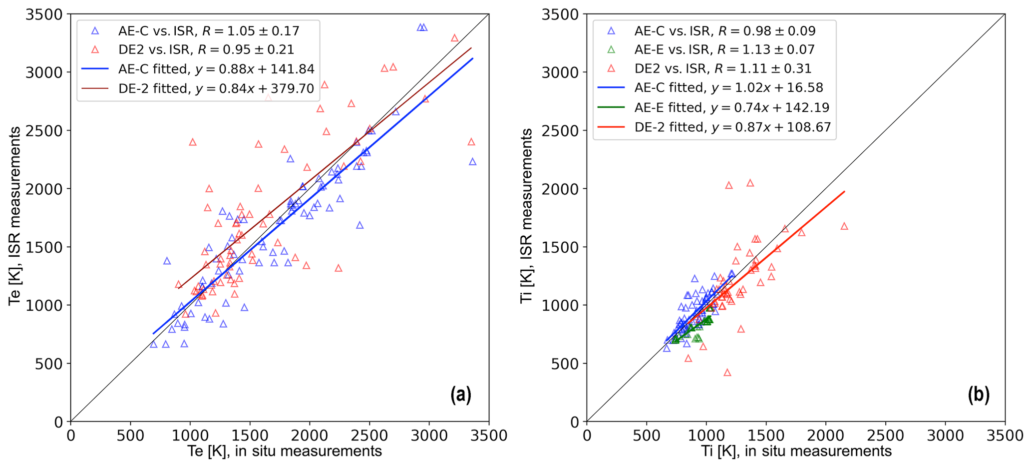
Figure 1 (a) Correlation between in situ measurements of T_e from AE-C (blue) and DE-2 (red) and corresponding ISR measurements, during times of conjunctions. (b) Correlation between T_i measurements between in situ measurements of AE-C (blue), AE-E (green) and DE-2 (red), during times of conjunctions with ISRs. Lines in both plots show linear fits. The linear fit parameters are marked in the insets of both plots.

The results shown in Fig. 1a and b indicate that AE-C and ISR data yield similar measurements for both T_e and T_i during their conjunctions. This is consistent with the findings of the study by Benson et al. (1977). Following the same approach and extending the work of Benson et al. (1977), Fig. 1a also presents T_e measurements from DE-2 and ISRs during times of conjunctions. The comparisons show that DE-2 measurements have a slope that is lower than 1, meaning that DE-2 systematically measures higher electron temperatures than the ISRs. It is noted that no conjugated measurements of T_e were found between AE-E and ISRs. Similarly, Fig. 1b presents T_i measurements from AE-E and DE-2 during times of their conjunctions with ISRs; the comparisons of both AE-E and DE-2 with ISRs during times of their conjunctions yield slopes that are lower than 1, meaning that both AE-E and DE-2 systematically report higher ion temperatures than the ISRs. This could indicate the need for systematic recalibration of AE-E and DE-2 measurements, whereby AE-E and DE-2 measurements might need to be systematically lowered.

In addition to the correlation between in situ and ISR measurements of T_e and T_i that is shown in Fig. 1, the comparative analysis was extended by estimating also the ratio between in situ and ISR measurements as a function of local time and absolute longitude and altitude; these results are included in Appendix Figs. A1 and A2 for T_e and T_i comparisons, respectively. Figures A1 and A2 are plotted in the same format as Fig. 2 of Benson et al. (1977), to allow for cross-comparisons with that study. The numbers in the lower right corner in each panel of Figs. A1 and A2 indicate the ratio between satellite and radar measurements. From Figs. A1 and A2 it can be seen that the conjunctions are well distributed over local time, absolute longitude separation between the satellites and radars, and altitude. Furthermore, in Figs. A1 and A2 we also plot the number of measurements as a function of the in situ (SAT) over radar (ISR) measurements in order to visualize the distribution of the measurements under comparison over local time, absolute longitude separation and altitude. The estimated linear fits in these figures are in agreement with the results from Benson et al. (1977), in particular for T_e for all satellites and T_i for AE-C and AE-D. However, a larger standard deviation is observed in the linear fit of T_i measurements from DE-2 with respect to the ISR measurements. This is more evident for high T_i, with satellite measurements appearing to underestimate T_i compared to ISRs. Finally, in Fig. A3 we plot histograms of measurements distribution over the calculated ratio. Figure A3 is plotted in the same format as Fig. 3 of Benson et al. (1977), allowing for comparisons between the two studies.

3 Comparisons between in situ ion and neutral temperatures

This section presents an analysis of the comparison between T_i and T_n as measured simultaneously on board satellites AE-C, AE-D, AE-E and DE-2, focusing in particular on the distribution in altitude, latitude and longitude of cases where T_i<T_n. The purpose of this analysis is to comment on the causes (either instrumental or physical) behind deviations from the commonly held perception that T_i is generally expected to be greater than T_n in the LTI.

3.1 Dataset

As a first step, from the entire database of T_i and T_n measurements obtained from satellites AE-C, AE-D, AE-E and DE-2, data were only considered when the satellites were located below 500 km. From this subset, all cases with simultaneously valid T_i and T_n measurements were selected. For the selection of valid data points, the WATS instrument data processing of DE-2 was followed (NASA, 1998). As part of this process, temperatures in the datasets were regarded as valid when the condition $\mathrm{200}\le T_k\le \mathrm{4000}$ was met, where $k=e,i,n$. After subtracting all data points flagged as erroneous, the dataset of temperature measurements where T_i and T_n are simultaneously valid consists of 52 822, 11 960, 171 775 and 236 785 data points for satellites AE-C, AE-D, AE-E and DE-2, respectively.

Subsequently, the subset of measurements when T_i<T_n was identified for each satellite. From this subset, only data points where T_i<T_n appeared at consecutive points along the orbit were considered, whereas individual (i.e., non-sequential or singleton) points were discarded. Within this dataset from satellites AE-C, AE-D, AE-E and DE-2, the condition that T_i<T_n was met in 18 959, 2934, 4501 and 10 674 data points, respectively, corresponding to 36 %, 25 %, 3 % and 5 % of the total numbers of valid data points, respectively. These numbers indicate that there is a non-negligible occurrence rate of cases when neutrals are (or appear to be) hotter that ions.

In the following we first present two examples of such events where the condition T_i<T_n is observed; we then proceed to investigate the statistical distributions of these events, both in altitude and in longitude vs. latitude.

3.2 Test cases of T_i<T_n events

An example of such an event occurred on 17 January 1975, during orbit 5089 of AE-C. An overview is shown in Fig. 2, where in the first three panels the spacecraft altitude, latitude and L shell are plotted, whereas in the fourth panel T_i and T_n are plotted in blue and green, respectively. Solar and geomagnetic indices during the time of this event were as follows: Dst ranged from −17 to −15 nT, the auroral electrojet (ae) index ranged from −172 to −62 and Kp ranged from 3+ to 4, indicating moderate geomagnetic activity levels.

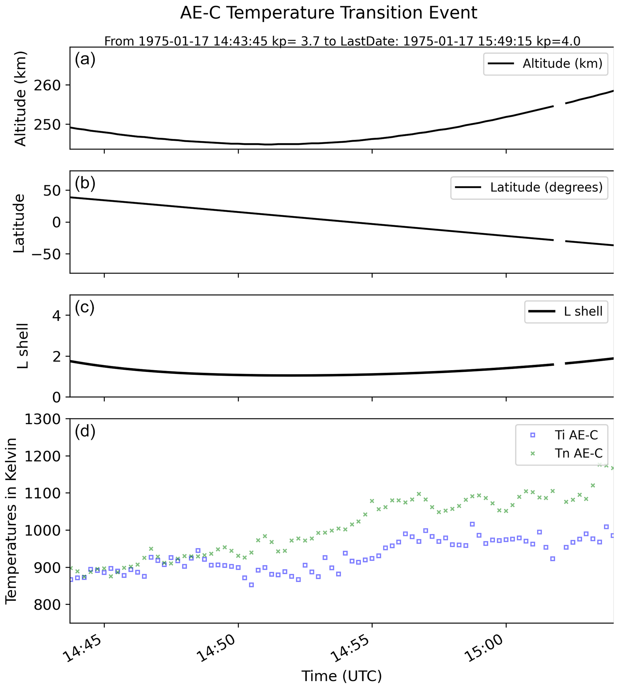
Figure 2 (a) Altitude, (b) geographic latitude, (c) L shell, and (d) T_i (blue) and T_n (green), for AE-C orbit no. 5089, on 17 January 1975, 14:43 to 15:49 UT.

The second example, plotted in Fig. 3, shows a sequence of five DE-2 orbits. During this event, the transition from T_i≥T_n (first orbit) to T_i<T_n (second to fifth orbits) is observed. Solar and geomagnetic indices during this time are as follows: Dst $=-\mathrm{44}$, ae =81, and Kp $=\mathrm{2}-$ to 4. This indicates low to moderate geomagnetic activity levels. It is noted that between each orbit there are data gaps in the DE-2 dataset.

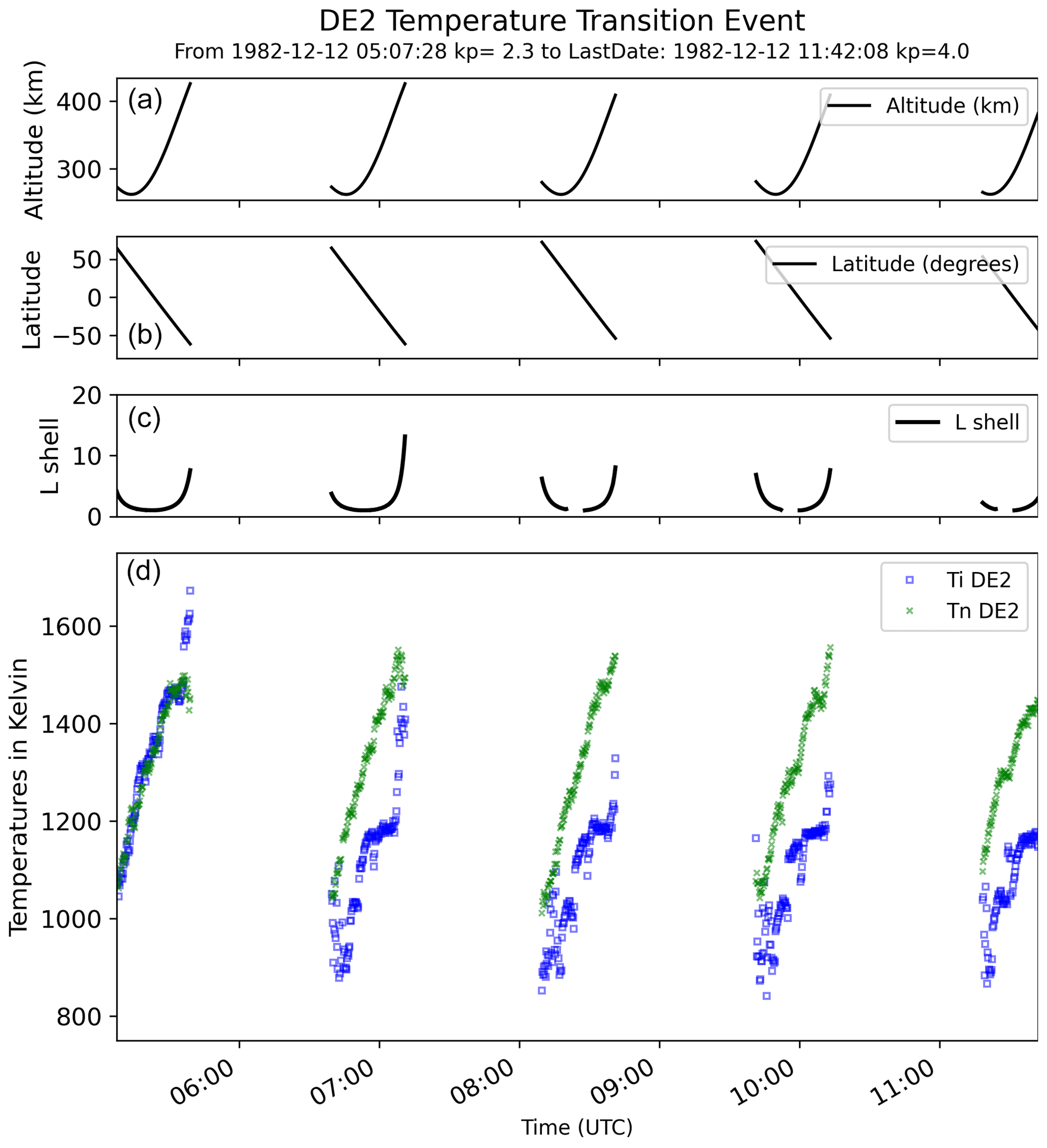
Figure 3 (a) Altitude, (b) geographic latitude, (c) L shell, and (d) T_i (blue) and T_n (green), for DE-2 orbits 7491 to 7495, on 12 December 1982, 05:07 to 11:42 UT.

The ground tracks of these events are shown in Fig. 5, where the ground track of the AE-C orbit of Fig. 2 is shown with a solid line, whereas the ground tracks of the five consecutive DE-2 orbits of Fig. 3 are shown with five dashed lines.

3.3 Spatial distribution of T_i<T_n cases

In Fig. 4 we plot all the occurrences of $\mathrm{\Delta }{T}_{\mathrm{in}}=T_{\mathrm{i}}-T_{\mathrm{n}}$ (both positive and negative) as a function of altitude, separately for each spacecraft. To this direction, panels (a) through (d) of Fig. 4 present the altitude distribution of all ΔT_in for AE-C, AE-D, AE-E and DE-2, respectively. The temperature of thermal equilibrium between ions and neutrals, or ΔT_in=0, is plotted with an orange line, whereas the local mean of ΔT_in is plotted with a light blue line; the local mean was calculated at altitude steps of 5 km. As it can be seen in these panels, whereas the local mean shows a positive average ΔT_in for all missions at all altitudes (with the exception of the lowermost altitudes of AE-C), there is a non-negligible number of cases where negative differences are observed. Furthermore, these plots show a positive trend of ΔT_in with altitude, meaning that cases of ΔT_in<0 are more likely to be observed at lower altitudes.

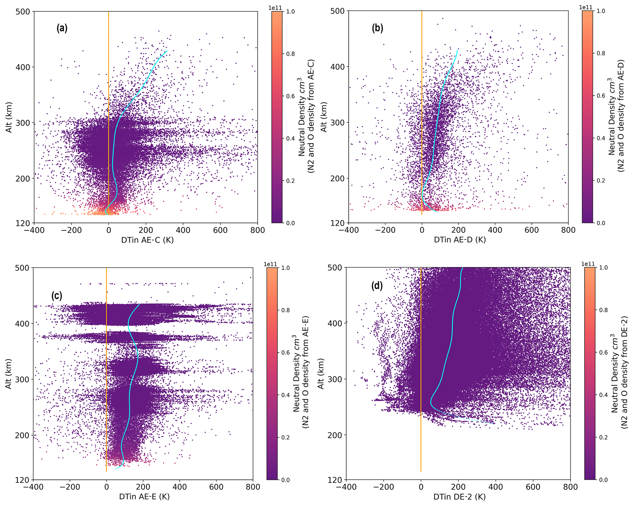
Figure 4 ΔT_in for the various satellite datasets, as marked. (a) ΔT_in vs. altitude (km) for AE-C, (b) ΔT_in vs. altitude (km) for AE-D, (c) ΔT_in vs. altitude (km) for AE-E and (d) ΔT_in vs. altitude (km) for DE-2. The color scale of the data points represents the neutral density, as obtained from the addition of N₂ and O in situ density measurements.

In Fig. 5 we plot the distribution of all cases where T_i<T_n (such as those shown in Figs. 2 and 3) as a function of geographic latitude and longitude. The geographic distribution of the T_i<T_n cases is depicted by plotting the corresponding probability distribution function (PDF) (Billingsley, 1986) of the occurrence of such events. The PDF is calculated based on the kernel density estimation (KDE) method (e.g., Rosenblatt, 1956; Scott, 1992; Rossini, 2000), using Gaussian kernels. More specifically, as part of the fundamental principle of a Gaussian KDE, each data point is given a Gaussian distribution (kernel), and these distributions are subsequently added up to produce a smooth approximation of the underlying probability density. The results are then normalized to produce the relative (unit-less) likelihood. The normalization is performed by subtracting the lowest value that is observed on the map from the PDF value at each point and subsequently dividing by the range from maximum to minimum PDF value; thus the resulting values range from 0 (corresponding to the lowest likelihood for the observation of T_i<T_n), which is marked as blue in Fig. 5, to 1 (corresponding to the highest likelihood), which is marked as red. In Fig. 5, the solid line marks the orbit of AE-C on 17 January 1975 that corresponds to the sample event shown in Fig. 2, and the five dashed lines mark the orbits of DE-2 on 12 December 1982 that correspond to the event shown in Fig. 3. Letters A through J indicate regions of interest that are discussed in further detail in the section below.

4 Discussion

In the following, we discuss possible reasons leading to the appearance and distribution of the occurrences of ΔT_in<0. Both potential instrumental or measurement effects and physical processes are discussed, including implications for our current understanding of LTI processes.

4.1 Possible sources of measurement errors

There are several potential sources of uncertainty that can lead to systematic and random errors in the in situ measurement of temperatures in space. The removal or correction of such errors has been the topic of multiple studies over the past decades (e.g., DeForest, 1972; Whipple, 1981; Hastings, 1995; Ergun et al., 2021; Hanley et al., 2021). These errors are primarily due to the high spacecraft velocity and the interaction of the spacecraft with the surrounding plasma and neutral environment. For example, factors that affect the accuracy of measuring ion temperatures include the acceleration of plasma by a charged surface, the generation of a complex plasma cloud that surrounds the spacecraft and interacts with the environment, and impact ionization and reflection of particles off the spacecraft and the subsequent inclusion of reflected ions in the measurements (e.g., Heelis and Hanson, 1998; Ergun et al., 2021; Hanley et al., 2021). In particular, Ergun et al. (2021) addressed spacecraft motion effects due to the creation of a wake in the Martian ionosphere and demonstrated the recalibration of the instrumentation on the Mars Atmosphere and Volatile EvolutioN (MAVEN) spacecraft (Jakosky et al., 2015) with the aid of kinetic solutions and published results from laboratory experiments, through which they achieved a significant improvement in the systematic uncertainty in T_e measurements. Similarly, Hanley et al. (2021) discussed a series of rigorous processes that they employed to identify and correct various sources of uncertainties in measurements of T_i arising from the supersonic velocities of MAVEN; these include altitude-dependent systematic errors as well as random errors from statistical fluctuations and uncertainties in spacecraft potential.

Based on the general agreement between in situ and ISR estimations of T_i, it is noted that T_i measurements are less likely than T_n to include large systematic deviations that could lead to the appearance of ΔT_in<0 in a statistically significant percentage of the total number of measurements, indicating that these measurements are less likely to be regarded as outliers. Factors affecting the accuracy of neutral temperature measurements include the applicability of the kinetic theory used in extracting neutral temperatures, in particular at lower altitudes where a shorter mean free path of the measured particles might affect the measurements, and gas–surface interactions, which are also dependent on altitude and neutral density (e.g., Spencer et al., 1973).

The altitude dependence that is shown by the light blue curves of Fig. 4 indicates that the appearance of ΔT_in<0 could be dependent on such spacecraft–environment interaction effects, which are expected to be dependent on neutral density. This effect could account for the larger appearance of ΔT_in<0 at altitudes below 150 km, as is shown, for example, in AE-C measurements; however, as it can be seen in Fig. 4a, in the altitude ranges from ∼ 150 to 200 km, there is a decrease in the appearance of such events, which are again enhanced at altitudes upwards of 200 km.

4.2 Possible physical mechanisms that could lead to observations of T_i<T_n

The structured appearance of the occurrence rates of the ΔT_in<0 events in Fig. 5 (as opposed to an even or random distribution of such events in latitude and longitude) indicates that there are, potentially, distinct underlying mechanisms leading to either the enhancement of neutral temperatures or the decrease in ion temperatures in these regions. In the following, the regions of enhanced probability for the appearance of ΔT_in<0 events are discussed, followed by a discussion on the possible underlying physical mechanisms that could be the cause of these observations. It is noted that the analysis presented herein is only meant to highlight these intriguing results and to point to potential mechanisms but cannot, at this point, yield a dominant mechanism or combination of mechanisms that can conclusively explain these results.

In Fig. 5, there are seven distinct regions of enhanced occurrences of ΔT_in<0 measurements; these are marked from A through G, as follows. There are four primary peaks of high occurrences, marked as A through D, that are located close to the geomagnetic equator. Of these, A and B are located in the South Atlantic and Indian oceans, respectively, whereas secondary peaks marked as C and D are observed in the western and eastern Pacific Ocean, respectively. A distinct enhancement is observed in the north Mexico/Baja California region and is marked as E. An enhancement is also observed in the northern Atlantic Ocean (as compared, e.g., to the continental regions of North America and Europe) and is marked as F. A distinct peak can be observed off the southern coast of Alaska and western Canada (compared to the corresponding continental regions) and is marked as G. Furthermore, there are four regions which have distinctly smaller concentrations of observations of ΔT_in<0 events: these are observed in the northern and southern high-latitude regions, which are marked as H; in the European continental region, which is marked as I; and in the northern Russian region, which is marked as J.

A first candidate mechanism that can significantly impact the LTI, altering neutral temperatures, concerns gravity waves (GWs). Gravity waves are dissipated in the thermosphere at altitudes between 100 and 200 km through molecular damping, modifying thermospheric temperatures (Walterscheid, 1981). Gravity waves generally form in the troposphere and lead to the transfer of momentum from the troposphere to the stratosphere and mesosphere and even further upwards to the thermosphere (Fritts and Alexander, 2003). These waves propagate upwards from the troposphere, and, in doing so, they grow exponentially in terms of wave amplitude (e.g., Andrews et al., 1987). The subsequent wave breaking of these large-amplitude waves leads to significant energy and momentum deposition. The detailed parameterization of GWs is an open issue in upper-atmosphere research, in particular for medium- (meso-β) and small-scale (or meso-γ) GWs, measurements of which are completely lacking (see, e.g., Liu, 2019) and whose effects could be significant for LTI energetics and dynamics.

The heating and cooling effects of GWs in the thermosphere have been extensively investigated by many simulation studies. For example, Yiğit and Medvedev (2009) used a GW parameterization that was specifically designed for thermospheric heights, which was implemented in the Coupled Middle Atmosphere and Thermosphere (CMAT2) global circulation model (Harris, 2001; Dobbin, 2005), covering altitudes from the tropopause to the F2 region. They performed simulations for the June solstice and illustrated the regions of GW heating and cooling rates. The simulation results indicated significant irreversible heating in the high latitudes of both hemispheres, which reached 90 to 100 K d⁻¹ near 200–210 km; secondary peaks in heating also appeared in the tropics, predominately below 130–140 km, which reached up to 10 K d⁻¹. Such preferential heating of the neutrals by GWs is compatible with the observations presented herein. However, even though regionally GWs can lead to significant heating in the thermosphere, Yiğit and Medvedev (2009) note that the net thermal effect of GWs is primarily cooling of the thermosphere and that the simulated model temperatures can be decreased by up to 200 K at the summer pole and by 100 to 170 K at other latitudes near 210 km. Simulations by England et al. (2020) also show that GWs can lead to cooling of the neutrals in the LTI at altitudes above 210 km.

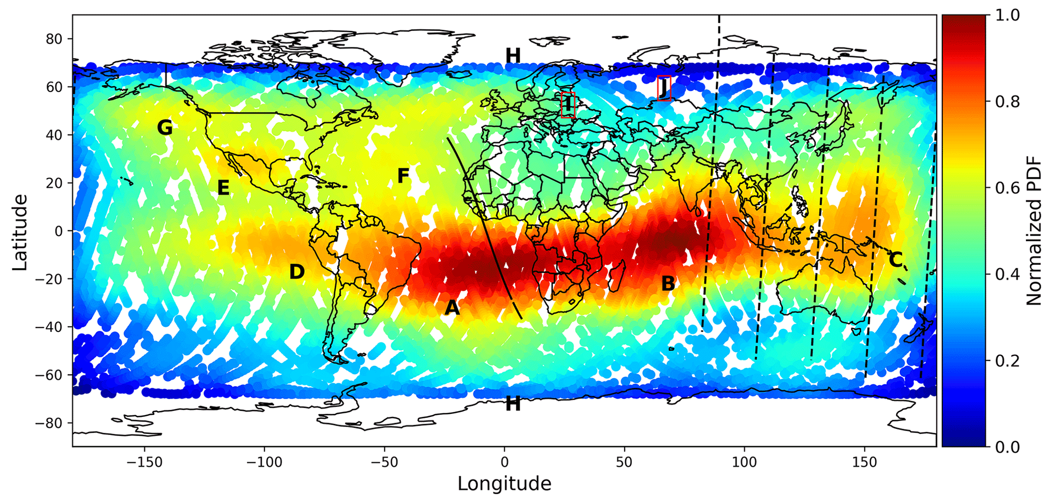
Figure 5 Probability of occurrence of ΔT_in<0 in AE-C measurements of T_i and T_n. The solid black line represents orbit no. 5089 of AE-C (Fig. 2), whereas the dashed black lines represent orbits nos. 7491 to 7495 of DE-2 shown in Fig. 3. The color scale represents the normalized probability distribution function, ranging from 0 (corresponding to the lowest likelihood for the observation of T_i<T_n), which is marked as blue, to 1 (corresponding to the highest likelihood), which is marked as red.

GWs can be generated through a range of different processes: these can be of meteorological origin (convective, shear, geostrophic) or topographic origin (e.g., mountain waves) or even due to strong tropospheric disturbances. In the following we discuss the generation mechanisms and localizations in relation to the appearance of ΔT_in<0 events.

Intense GWs are known to be generated by winds flowing over mountain formations; for example, Hierro et al. (2018) reported the appearance of GWs over the Andes. However, whereas peak D could possibly be associated with the Andes, there are no corresponding signals over North America (Rocky Mountains), Europe (Alps) or India/China (Himalayas); this indicates that there is possibly no clear association of ΔT_in<0 events with GWs of topographic origin.

Together with mountain ranges, GWs are known to be generated by hurricanes, typhoons and tropical cyclones. In order to find potential correlations with such dynamical tropospheric events, all relevant occurrences of hurricanes, typhoons and tropical cyclones combined were collected from the NOAA IBTrACS v4 (Knapp et al., 2010, 2018) database and are plotted in Fig. A4 for the time period from 1974 to 1976 corresponding to the period of in situ measurements that are plotted in Fig. 5. It is noted that the region marked as E and F in Fig. 5, and in particular the region extending from $\sim \mathrm{18}{}^{\circ }$ N to $\sim \mathrm{40}{}^{\circ }$ N and $\sim \mathrm{120}{}^{\circ }$ W to $\sim \mathrm{80}{}^{\circ }$ W, has a particularly high occurrence rate of hurricanes and typhoons and a markedly similar extent in their localizations. The same is observed in the region of the Indian Ocean and north of Australia, from $\sim \mathrm{10}{}^{\circ }$ N to $\sim \mathrm{40}{}^{\circ }$ S and ∼ 40^∘ E to ∼ 150^∘ E, which has a particularly high occurrence rate of tropical cyclones. However, no such events are observed over the regions marked as A, B and D, meaning that different mechanisms are taking place in these regions.

Together with the above regions of dynamical tropospheric events, such as hurricanes, typhoons and cyclones, and the appearance of GWs in association with large mountain formations, there are many other triggers of highly localized and persistent GWs: for example, such phenomenology has been termed a “GW hot spot”, appearing over specific regions and times (e.g., Becker et al., 2022). Other studies have reported the lack of GWs over specific regions: for example, resulting from the diurnal tide's strong poleward winds over the European area, some GWs were found to be moving westward across the Atlantic and eastward over eastern Europe (e.g., Becker et al., 2022), leaving a gap in terms of GW occurrence over Europe. Investigating in detail the appearances of these localizations and their causes is a topic that is beyond the scope of this paper and that is left for future studies.

Recently, Vadas and Azeem (2021) reported on GWs that can cause up to 75^∘ K changes at 200 km. Interestingly, they report that the locations of these GWs, even though orographically generated, are not centered on mountains but instead radiate from them. They also reported that these GWs are attenuated by horizontal magnetic fields and that they could be located 1 or 2 d after a large polar vortex event. These results indicate that the correlation between the generation mechanism, the region and the effects of GWs can be a much more complicated process than currently thought.

Another potential mechanism that could lead to an enhancement of T_n and hence to the appearance of instances of ΔT_in<0 could be associated with the equatorial region fountain effect: during this process, the plasma is driven upwards due to an E×B drift, owing to the eastward direction of E and the northward (parallel to the Earth's surface) direction of B. The plasma motion drives the neutral gas to move upwards as well, through the momentum transferred via collisions between neutral and charged particles, transferring momentum from the plasma to the neutral gas. These collisions end up heating the neutral gas, whose temperature is gradually enhanced. At higher altitudes, the E×B drift stops driving the plasma upwards, which, in the absence of an electric field, follows the magnetic field lines, mapping to latitudes northwards and southwards of the magnetic equator. This process leaves the heated neutrals with an average temperature T_n that is higher than the ion temperature T_i.

An additional candidate mechanism that could lead to the appearance of ΔT_in<0 is related to the South Atlantic Anomaly (SAA), the region over the South Atlantic Ocean where the magnetic field strength is significantly weaker than in other parts of the planet (Vernov and Chudakov, 1960; Yoshida et al., 1960; Ginzburg et al., 1962): the low altitude of the mirroring point of energetic particles in this region leads to enhanced fluxes of precipitating high-energy ions and electrons that are higher than at other longitudes. This leads to enhanced collisions with the neutrals, and since the early days of space exploration it has been speculated that this can lead to the deposition of a significant amount of energy to the neutral atmosphere. Indications that the neutral temperatures could be higher in the SAA region than elsewhere were provided early on, e.g., by Wulff and Gledhill (1974) and Gledhill (1976) and references therein.

Instrumental/measurement effects are also known to be correlated to the SAA: for example, it is known that penetrating high-energy particles can introduce enhanced noise in most instruments. This could be seen as enhanced background noise on the T_i signal as obtained from the RPA instrument or the T_n signal from the NATE instrument or in both signals.

From the results shown in Fig. 5 it is noted that, whereas the region of primary enhancement of the occurrence rates of ΔT_in<0, marked as A, reaches the vicinity of the SAA, its peak is offset in terms of latitude and longitude to the northeast of the SAA; furthermore, it is noted that the SAA region is more restricted in latitude than the region of observations. Finally, plotting the same data shown Fig. 5 binned by altitude does not indicate a trend in altitude (results not shown herein). For example, SAA signatures would be expected to become more intense and restricted in longitude at low altitudes; hence an increase in the occurrence rates of ΔT_in<0 with decreasing altitude would signify a correlation with the SAA, which has not been identified herein. Further complicating the interpretation of these results, the appearance of the second largest peak in the occurrence rates of ΔT_in<0 in the vicinity of the Indian Ocean, marked as B in Fig. 5, cannot be attributed to or be associated with the SAA.

Another mechanism that could significantly affect the dynamics and energetics of the thermosphere is related to the as yet unresolved phenomenon of the ionospheric plasma caves, the unusual decreases in electron density that are theoretically expected to occur in the equatorial regions. For example, Liu et al. (2010), Lee et al. (2012) and Chen et al. (2014) presented theoretical studies of the equatorial ionization anomaly region's ionospheric plasma cave based on FORMOSAT-3/COSMIC and Dynamic Explorer 2 (DE-2) and simulations, respectively. The plasma cave structures are attributed to neutral winds that are distinguished by two divergent wind zones at off-Equator latitudes and a convergent wind region at the magnetic equator. Since electrons mainly transfer energy to the ions, the absence of electrons within plasma caves is speculated to create the conditions for the occurrences of neutrals that are hotter than ion. Plasma caves are expected through simulations to be observed between ∼ 0–$\sim \mathrm{120}{}^{\circ }$ E, which is in rough agreement with the peaks marked as A and B in Fig. 5, over the South Atlantic region. They are also expected to show a significant latitudinal asymmetry, which is also observed in Fig. 5. However, as noted in Chen et al. (2014), there are considerable remaining discrepancies between simulations and observations of plasma caves, primarily due to unknowns in the distribution and structuring of neutral winds in the lower-thermospheric altitudes.

Together with the above analysis that compares the temperatures of ions and neutrals in the ionosphere–thermosphere, the relative temperature of electrons and ions is of extreme importance to the state of the ionosphere. Whereas globally it is expected that it is much more common for T_e to be greater than T_i due to the effects of UV radiation, at times T_i>T_e has also been observed, associated with storm-time-enhanced joule heating. For example, through analyzing EISCAT ISR data, Kofman and Lathuillere (1987) have shown profiles of very high ion temperatures (greater than 8000 K), observed along geomagnetic field lines, which they attributed to frictional heating between fast-moving species. Similarly, Buchert and Hoz (1988) also reported observations of very high ion temperatures (on the order of 12 000 K), which were not accompanied by commensurate changes in the electron temperature; they also attributed such cases of T_i<T_e to joule heating. Although believed to be less common, such events are expected to be energetically very significant. Such events are not analyzed statistically herein and are the topic of a future study.

5 Summary and conclusions

In this study, a comparison between in situ satellite (AE-C, AE-E and DE-2) and ISR (Arecibo, Millstone Hill and St Santin) measurements of T_e and T_i has been performed. Through this comparison, it has been found that the agreement between satellite and ISR measurements is best for AE-C and AE-E for both T_e and T_i and is quantitatively similar to the results of Benson et al. (1977) that focused on only AE-C measurements. The results presented herein show a larger discrepancy for DE-2, both in terms of the fits to the data and to the standard deviation, and indicate that DE-2 possibly overestimates T_i, with deviations being higher for higher temperatures.

Through a re-analysis of ion and neutral temperatures, a surprisingly high occurrence rate of ΔT_in<0 is reported. Furthermore, an intriguing spatial distribution of the occurrences of ΔT_in<0 is presented, showing distinct peaks in the occurrence rates in (in order of significance) (a) the South Atlantic Ocean, (b) the Indian Ocean, (c) the southwestern Pacific Ocean, (d) the eastern Pacific Ocean, (e) north Mexico/Baja California, (f) the northern Atlantic Ocean and (g) the northeastern Pacific Ocean. A distinct lack of occurrences is observed (h) at all northern and southern high latitudes, (i) over Europe and northern Africa, and (j) over northern Russia.

Several potential causes have been identified that could explain the appearance of ΔT_in<0; these are summarized as follows:

• A ram cloud could produce ion temperatures that are cooler than the ambient neutrals; the deviation would be a function of neutral density. These clouds could be observed at all latitudes and longitudes, at low altitudes. Detailed instrument-level simulations are needed to accurately subtract ram cloud effects from measurements.

• Gravity waves (GWs) can have significant thermal effects, leading to localized heating of the neutrals but also to cooling. The parameterization of GWs and their distribution and occurrence, which are currently largely missing, will enable the exact quantification of their effects in terms of heating and cooling in the LTI.

• Precipitating particles in the South Atlantic Anomaly (SAA) can lead to an enhancement of neutral temperatures. The parameterization and localization of these effects require detailed simulations.

• Plasma caves, the regions where the unusual decrease in electron density is observed (Liu et al., 2010; Chen et al., 2014), can lead to a decrease in ion temperatures. Detailed simulations combined with in situ measurements of all relevant parameters could help resolve the regional and global effects of plasma caves.

• The equatorial region fountain effect, via the collisions between charged and neutral particles and the subsequent transfer of energy and momentum from the plasma to the neutral gas, is also a candidate mechanism. Detailed simulations combined with in situ measurements of all relevant parameters will help resolve the contributions of this effect on regional and global scales.

Whereas a single process cannot be invoked to explain the spatial distribution of the occurrences of observations of T_i<T_n, it is possible that different causes can be at play in different regions and/or at different times. Whereas instrumental effects cannot be excluded, the reported spatial distributions indicate that there are patterns in the occurrences of these events that hint at distinct underlying mechanisms that lead to either unexpectedly cool ion temperatures or unexpectedly warm neutral temperatures. It is noted that existing models cannot predict such observations of T_i<T_n, which highlights a lack of understanding of the underlying processes in the LTI. Recently, Peterson et al. (2023) also reported the appearance of cases where ΔT_in<0 and similarly concluded that there is so little that we know about the processes taking place in the LTI region and that, if ΔT_in<0 observations are real, they would emerge from unforeseen and unstudied physical processes; they also attributed such occurrences to high-altitude gravity waves (England et al., 2020).

The results presented herein are based on a re-analysis of the only available in situ co-spatial and co-temporal datasets of T_i and T_n, from the early Atmosphere Explorer and Dynamics Explorer missions, with the exception of a few rocket flights. Even though non-conclusive, these results highlight the fact that the LTI region is one of the least explored regions of the Earth's atmosphere and that there is very limited knowledge about the ongoing processes. It also highlights the limitations of current observational techniques, such as ISRs, which cannot simultaneously provide information about T_e, T_i and T_n. It is noted that observations of T_n in the lower thermosphere have also been provided via spaceborne UV instruments, such as GUVI on the TIMED satellite (Christensen et al., 2003), which could be combined with remote sensing of T_e and T_i from ISR measurements; for example, recently, Peterson et al. (2023) presented examples of co-temporal and co-spatial observations of T_n from GUVI as well as T_e and T_i observations from incoherent scatter radars. In their conclusions, they point out that the error bars on the presented temperature profile observations do not allow a strong conclusion to be drawn; however, a systematic statistical investigation of these combined datasets could yield more insight into the conditions leading to observations of ΔT_in<0.

In conclusion, it is noted that the combined and systematic measurement of all three T_e, T_i and T_n, ideally provided in situ from instruments on board the same platform, would allow us to make a conclusive statement on the thermal equilibrium between electrons, ions and neutrals and to investigate the regions and causes of deviations from that state. Several studies have highlighted the need for comprehensive in situ measurements to address key unknowns in this region (e.g., Sarris, 2019; Sarris et al., 2020; Palmroth et al., 2021; Sarris et al., 2023); by providing significantly larger volumes of measurements than are currently available, such in situ missions will greatly enhance our understanding of the LTI region, including the underlying causes of the observations of T_i<T_n.

Appendix A

Table A1 Orbit points and temperature measurements.

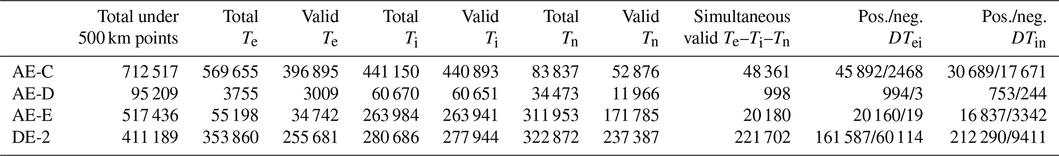
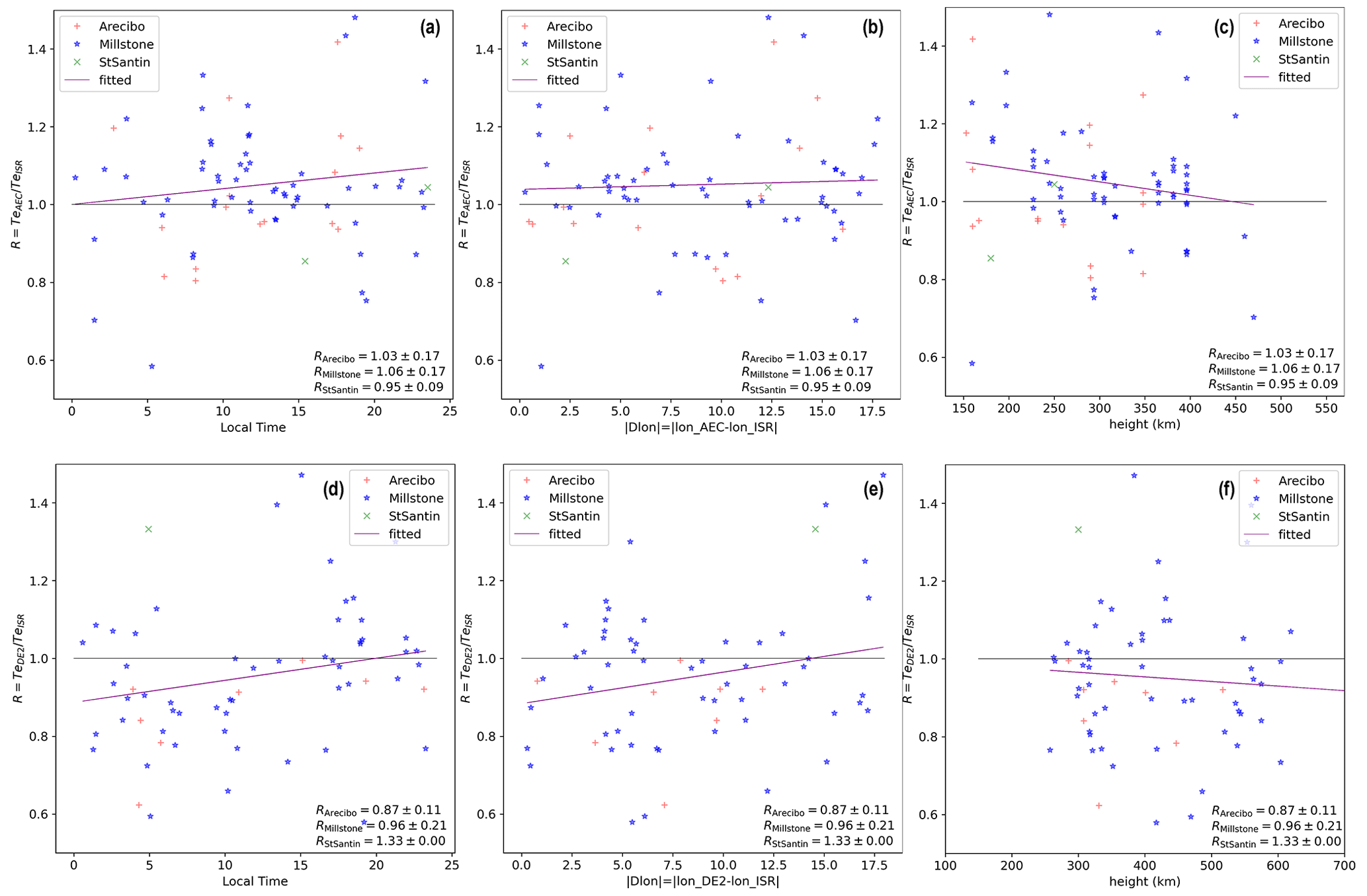
Figure A1 T_e ratio as a function of local time, absolute longitude separation and height for AE-C and DE-2 and ISRs. (a) AE-C T_e ratio as a function of local time, (b) AE-C T_e ratio as a function of absolute longitude separation, (c) AE-C T_e ratio as a function of height, (d) DE-2 T_e ratio as a function of local time, (e) DE-2 T_e ratio as a function of absolute longitude separation and (f) DE-2 T_e ratio as a function of height.

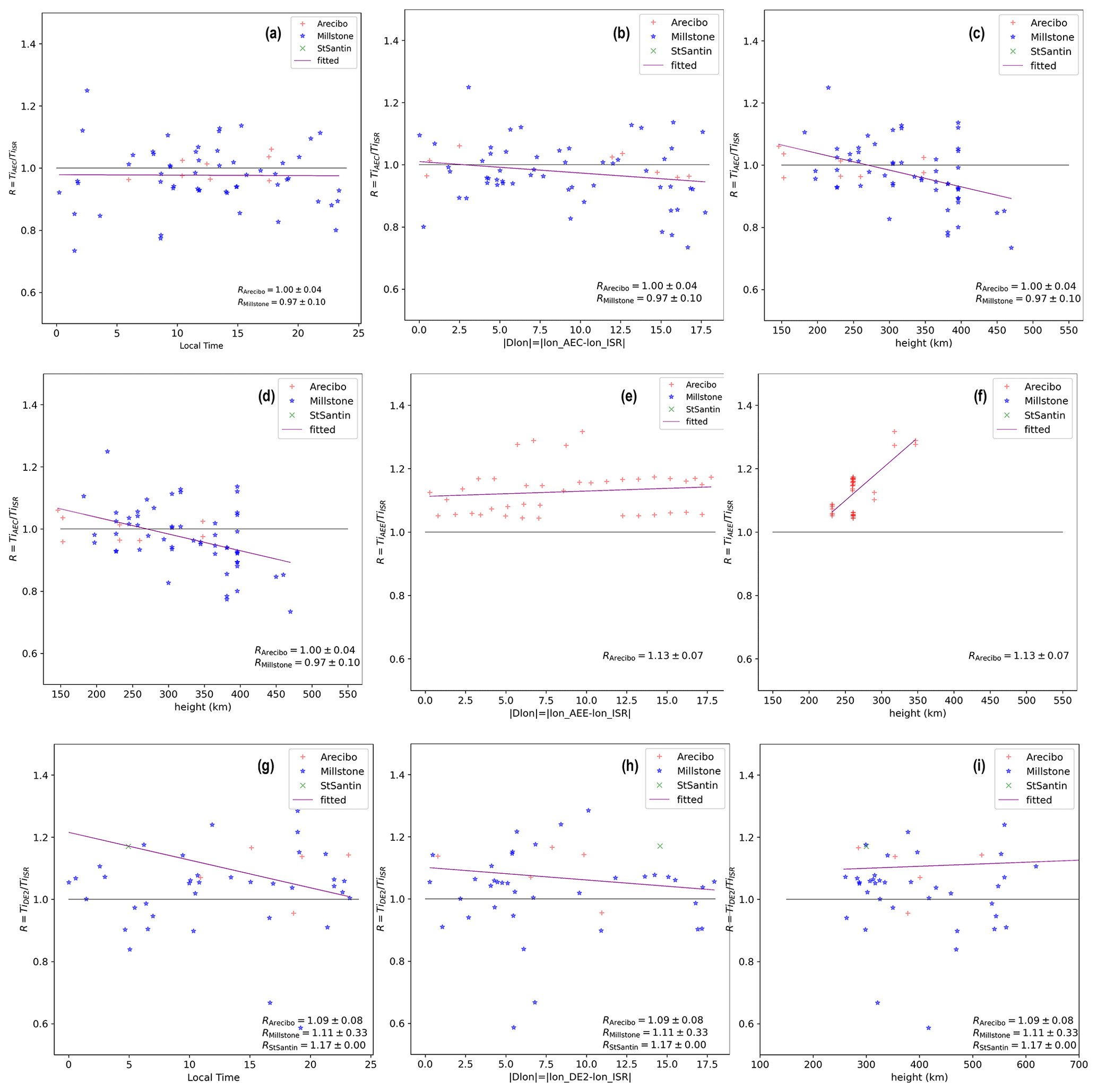
Figure A2 T_i ratio as a function of local time, absolute longitude separation and height for AE-C and ISRs. (a) AE-C T_i ratio as a function of local time, (b) AE-C T_i ratio as a function of absolute longitude separation, (c) AE-C T_i ratio as a function of height, (d) AE-E T_i ratio as a function of local time, (e) AE-E T_i ratio as a function of absolute longitude separation, (f) AE-E T_i ratio as a function of height, (g) DE-2 T_i ratio as a function of local time, (h) DE-2 T_i ratio as a function of absolute longitude separation and (i) DE-2 T_i ratio as a function of height.

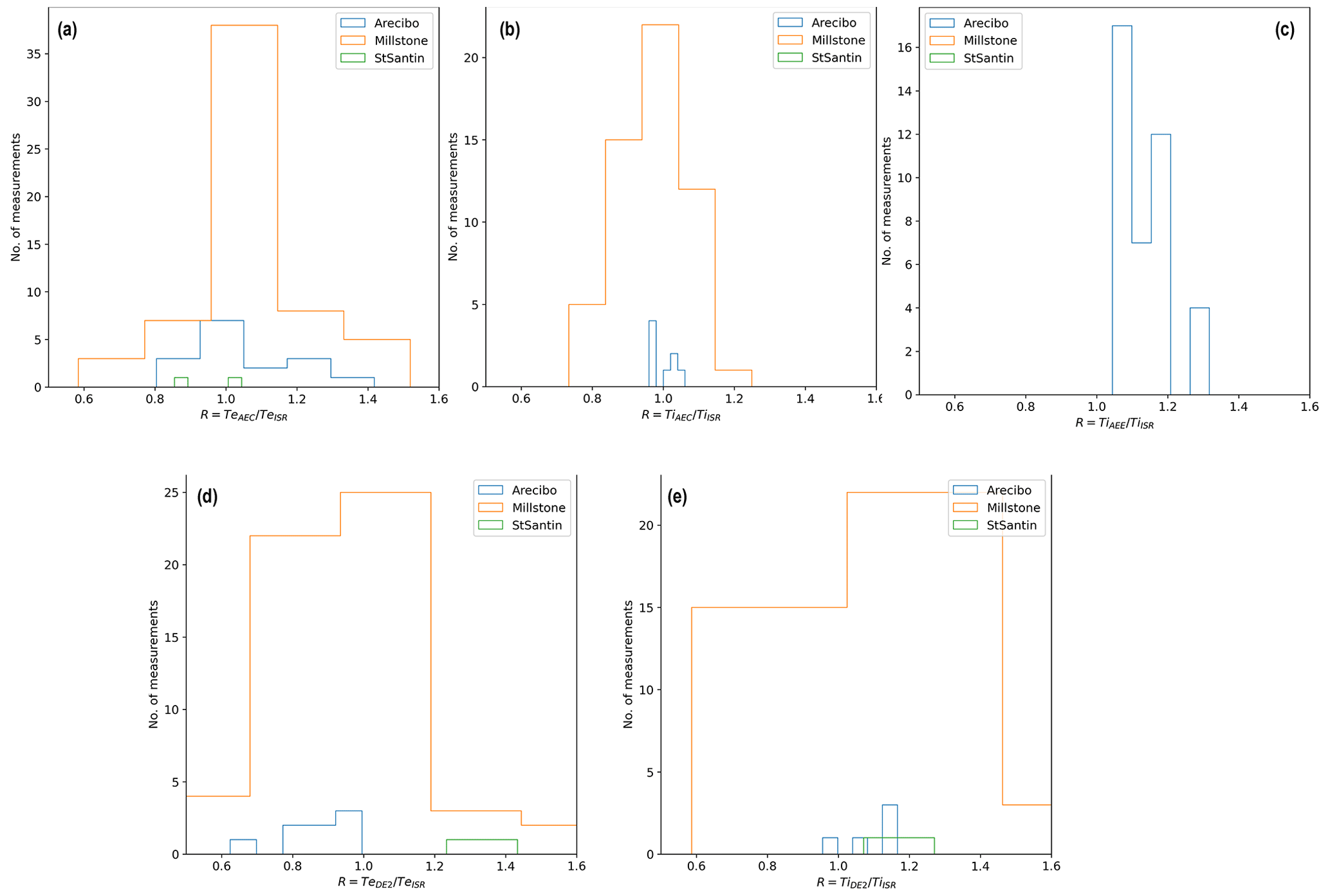
Figure A3 Distribution of satellites vs. ISR ratios. (a) AE-C T_e ratio, (b) AE-C T_i ratio, (c) AE-E T_i ratio, (d) DE-2 T_e ratio and (e) DE-2 T_i ratio.

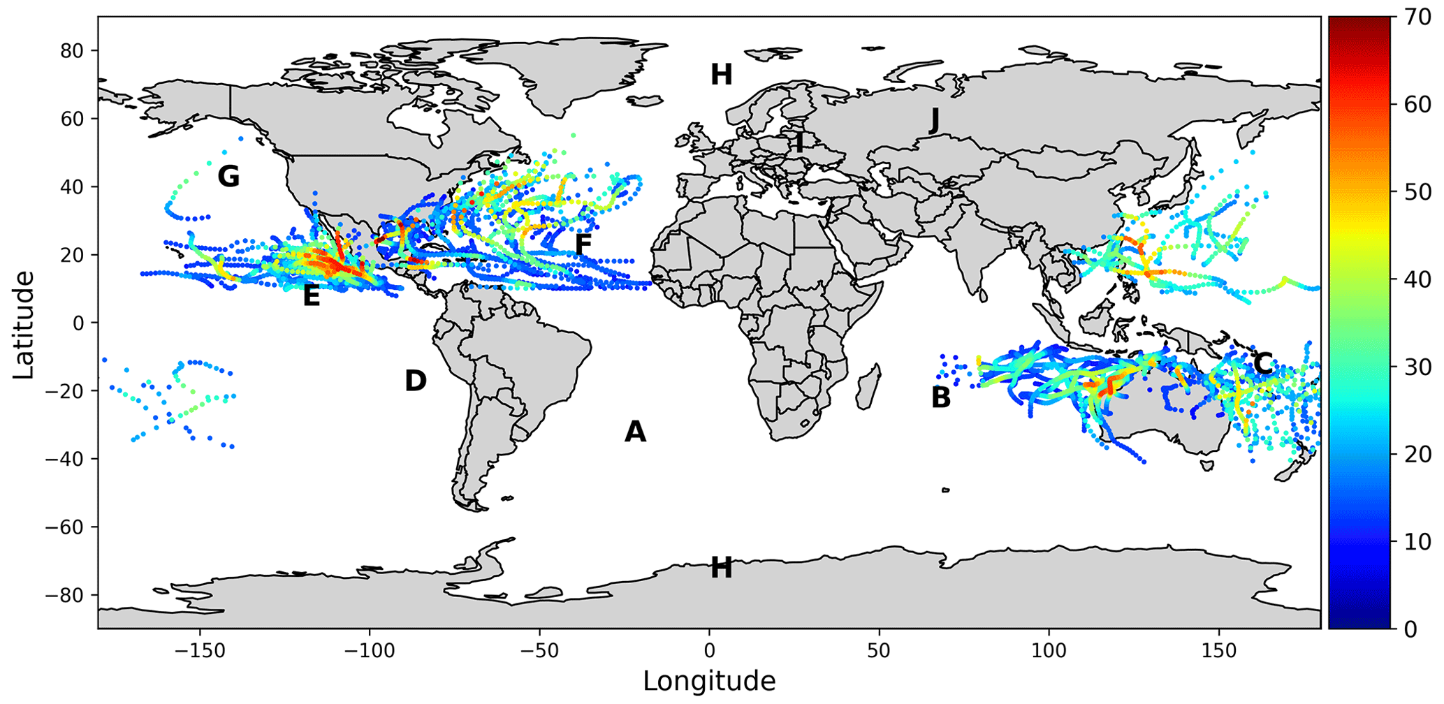
Figure A4 Typhoon and tropical cyclones between 1974 and 1978; color scale in meters per second.