Greenhouse gas effects on the solar cycle response of water vapour and noctilucent clouds

The responses of water vapour (H₂O) and noctilucent clouds (NLCs) to the solar cycle are studied using the Leibniz Institute for Middle Atmosphere (LIMA) model and the Mesospheric Ice Microphysics And tranSport (MIMAS) model. NLCs are sensitive to the solar cycle because their formation depends on background temperature and the H₂O concentration. The solar cycle affects the H₂O concentration in the upper mesosphere mainly in two ways: directly through the photolysis and, at the time and place of NLC formation, indirectly through temperature changes. We found that H₂O concentration correlates positively with the temperature changes due to the solar cycle at altitudes above about 82 km, where NLCs form. The photolysis effect leads to an anti-correlation of H₂O concentration and solar Lyman-α radiation, which gets even more pronounced at altitudes below ∼ 83 km when NLCs are present. We studied the H₂O response to Lyman-α variability for the period 1992 to 2018, including the two most recent solar cycles. The amplitude of Lyman-α variation decreased by about 40 % in the period 2005 to 2018 compared to the preceding solar cycle, resulting in a lower H₂O response in the late period. We investigated the effect of increasing greenhouse gases (GHGs) on the H₂O response throughout the solar cycle by performing model runs with and without increases in carbon dioxide (CO₂) and methane (CH₄). The increase of methane and carbon dioxide amplifies the response of water vapour to the solar variability. Applying the geometry of satellite observations, we find a missing response when averaging over altitudes of 80 to 85 km, where H₂O has a positive response and a negative response (depending on altitude), which largely cancel each other out. One main finding is that, during NLCs, the solar cycle response of H₂O strongly depends on altitude.

1 Introduction

The 11-year solar cycle significantly influences the upper-atmosphere's temperature and water vapour (H₂O) concentration. H₂O is one of the essential minor constituents in the mesosphere as it is the primary source of chemically active hydrogen radicals, influencing the chemistry of all other chemically active minor constituents (Brasseur and Solomon, 2005; Hartogh et al., 2010). H₂O concentration plays an essential role in the noctilucent cloud's (NLC) formation. NLCs are located at about 83 km altitude, consist of water ice particles, and owe their existence to the cold-summer mesopause region (∼ 130 K) at middle and high latitudes. NLCs, also called polar mesospheric clouds, are formed in an environment where small changes in background H₂O and temperature can lead to significant changes in NLC properties (e.g. Thomas, 1996; DeLand et al., 2006; Shettle et al., 2009; Lübken et al., 2009).

In comparison to the lower atmosphere, little is known about the upper mesosphere–lower thermosphere (MLT, 75–110 km) due to a lack of observations at these altitudes. NLCs have been proposed as indicators of trends in background temperature and H₂O concentrations (Thomas and Olivero, 2001). Studying NLC properties provides insight into phenomena occurring at the altitude of NLCs. The 11-year solar cycle has been considered to cause quasi-decadal oscillation observed in NLCs (DeLand et al., 2003). NLCs are predicted to decrease during solar maximum due to increased heating and photolysis of H₂O (Garcia, 1989). However, some recent studies strongly suggest that the response of NLCs to the solar cycle has been absent from 2002 to the present (Fiedler et al., 2011; DeLand and Thomas, 2015; Hervig et al., 2016; Siskind et al., 2013). Hervig et al. (2019), using satellite observations, found that NLCs had a clear anti-correlation with the solar cycle before 2002, and that response has been absent in recent years. The leading cause of this absence appears to be the suppression of the solar cycle response of H₂O. Lyman-α (Lyα) radiation is the primary cause of H₂O photolysis and varies by a factor of 2 between solar minimum and maximum (Woods et al., 2000). Understanding the effects of the solar cycle on H₂O is more complicated at NLC altitudes because of the interaction between NLCs and background H₂O.

NLC growth leads to dehydration at higher altitudes (83–89 km) as ice particles are formed by consuming background H₂O, and sublimation of ice particles leads to hydration at lower altitudes as H₂O is released here (about 78–83 km) (Lübken et al., 2009; Hervig et al., 2003). Investigating the effects of NLCs on the background H₂O requires an estimate of the H₂O profile without NLCs. Investigations using satellite observations are limited due to uncertainty in the inferred background H₂O without NLC and vertical resolutions on the order of a few 100 m. Therefore, using satellite observations to study H₂O at NLC altitudes could yield misleading results due to biases in the estimated H₂O profiles without NLC (Hervig et al., 2015). Hervig et al. (2015) suggest that, in future studies, one approach to investigate the effects of NLC on H₂O would be to use a detailed microphysical NLC model. Therefore, for this study, simulations are performed with and without microphysics using the same background conditions, resulting in an H₂O profile with and without NLC. This allows us to investigate how NLC formation changes the H₂O background profile in detail.

We compare the model result to satellite observations published by Hervig et al. (2019) to investigate the mechanism behind the solar cycle response of NLC and H₂O. We also focus on the missing solar cycle response of H₂O during recent years. This paper aims to answer a number of questions. How does the formation of NLCs affect the H₂O profile and the variation of water vapour with the solar cycle? How do the solar-cycle-induced temperature and photolysis changes affect the H₂O response? Why is the response of water vapour to the solar cycle nearly absent in satellite observations after 2005 (Hervig et al., 2019)? Our study is focused on the core NLC period, i.e. July at 68 ± 5^∘ N. The following section describes the modelling framework of this study and discusses the various model simulations performed. The third section discusses the mechanisms behind the solar cycle H₂O response, such as the separation of the solar-cycle-induced temperature and photolysis effects on H₂O. Sections 4 and 5 explore the possible reasons behind the missing solar cycle response. Concluding remarks and a summary are given in the last section.

2 Model description and numerical experiments

2.1 Model

The modelling framework used in this study consists mainly of two components: the Leibniz Institute Middle Atmosphere (LIMA) model and the Mesospheric Ice Microphysics And tranSport (MIMAS) model (see Fig. 1). LIMA is a non-linear, global, 3D Eulerian grid point model reaching from the troposphere to the lower thermosphere which calculates winds and temperature and is well described in a number of papers (Berger, 2008; Lübken et al., 2013). The LIMA model in this study is nudged to reanalysis data from NOAA-CIRES (National Oceanic and Atmospheric Administration-Cooperative Institute for Research in Environmental Sciences 20CR; Compo et al., 2011) up to an altitude of 45 km. The resulting winds and temperatures in the mesosphere and lower thermosphere (MLT) are then used in MIMAS. The MIMAS model run was performed for all years with background wind conditions and gravity wave forcing from a representative year (1976).

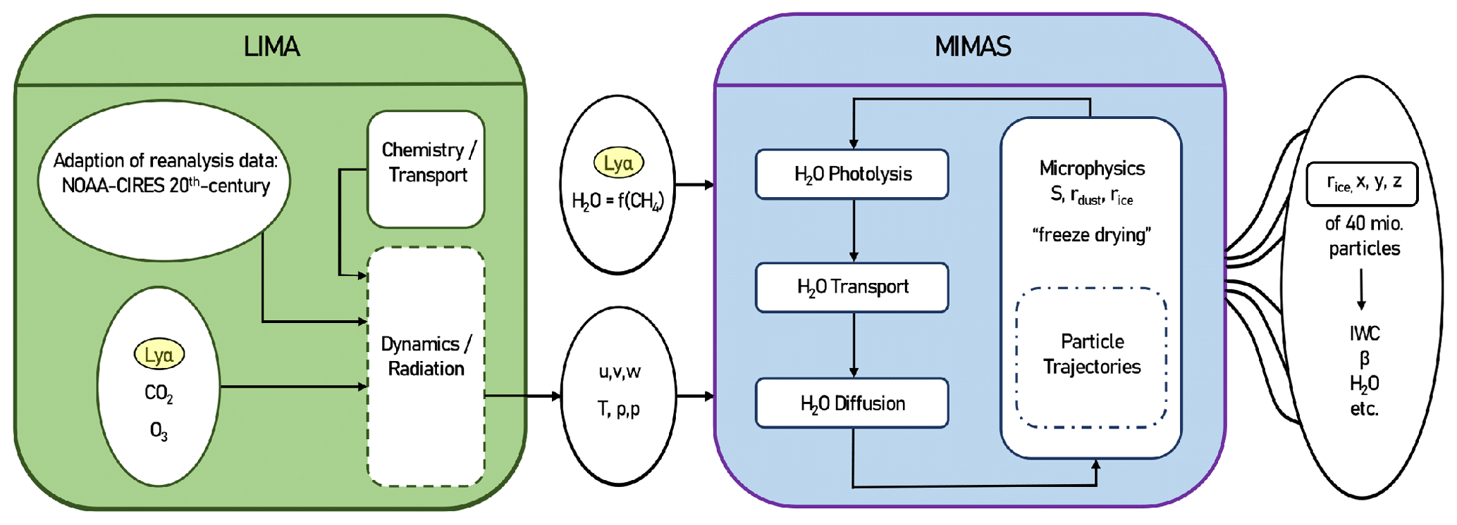
Figure 1 Sketch of the LIMA (green) and MIMAS (blue) models (from Lübken et al., 2021).

MIMAS is a 3D Lagrangian transport model specifically designed for modelling ice particles in the MLT region (Berger and Lübken, 2015). MIMAS calculates NLC parameters from 10 May to 31 August, and it is constrained from middle latitudes to high latitudes (37–90^∘ N) with a horizontal grid resolution of 1^∘ in latitude and 3^∘ in longitude and a vertical resolution of 100 m from 77.8 to 94.1 km (163 levels). In this study, the dynamics calculated by LIMA, solar Lyα, and the initial H₂O distribution are the input for MIMAS, as sketched in Fig. 1. Below the MIMAS lower boundary, two effects determine the mixing ratio of H₂O in the stratosphere: (i) transport of H₂O from the troposphere and (ii) oxidation of methane (CH₄). The oxidation of each CH₄ molecule produces two H₂O molecules. Methane is nearly completely converted to H₂O in the mesosphere by photochemical processes (e.g. Lübken et al., 2018). MIMAS assumes that transport from the troposphere is constant. The increase in H₂O is primarily through (ii), i.e. due to the increase in CH₄ concentration (Lübken et al., 2018). Then, mesospheric H₂O in MIMAS is transported by background winds, dispersed by turbulent diffusion, and reduced by photolysis. Hence, we parametrize H₂O as a function of CH₄ following Lübken et al. (2018) (see Sect. 2). MIMAS makes use of 40 million dust particles, which can act as condensation nuclei. Dust particles are formed from meteors evaporating in the atmosphere (for more details, see Berger and von Zahn, 2002; von Zahn and Berger, 2003; Killiani, 2014). These are then coated with ice in H₂O-supersaturated regions and transported according to three-dimensional and time-dependent background winds, eddy diffusion, and sedimentation. In MIMAS, standard microphysical processes such as the Kelvin effect determine the nucleation and growth of ice particles (Berger and Lübken, 2015; Gadsden and Schröder, 1989). For the comparison with satellites, we used model run A, which includes CO₂ and CH₄ variations (Lübken et al., 2018, 2021). We performed MIMAS model simulations with ice formation turned off and on respectively to investigate the effects of ice formation on background H₂O. In both runs, the background conditions and model inputs are the same. The main outputs of the model are the microphysical properties of the NLC ice particles, such as radius, backscatter value, and the number density of the ice and dust particles. More detailed descriptions of the MIMAS model and its precursors are available in the literature (Berger and von Zahn, 2002; Berger, 2008; Berger and Lübken, 2011; Lübken et al., 2018, 2021).

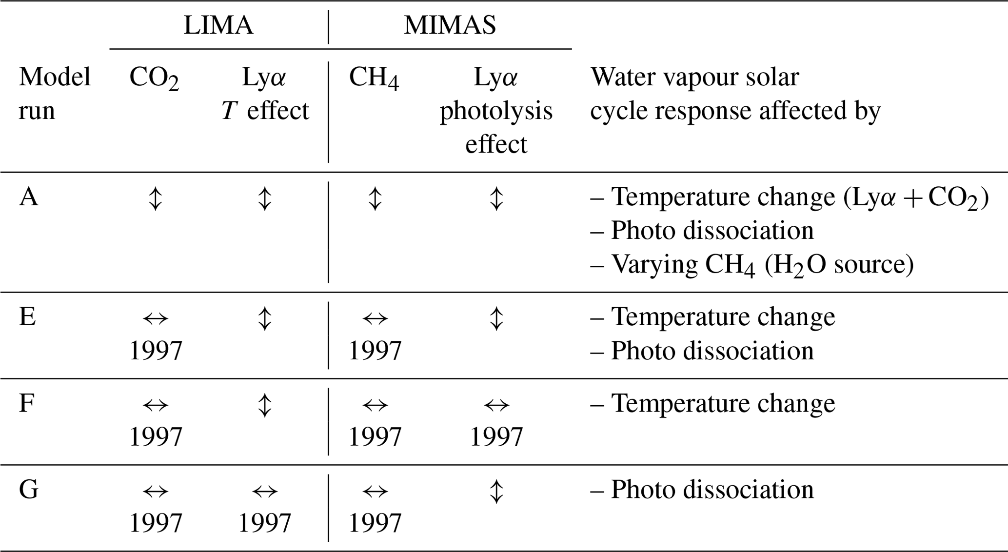
2.2 Model simulations

LIMA and MIMAS use daily Lyα fluxes taken from the LASP Interactive Solar Irradiance Data Center (LISIRD) as a proxy for solar activity from 1961 to 2019 (Machol et al., 2019). Lyα (and other spectral band) variations in LIMA cause atmospheric temperature variations, while Lyα variations in MIMAS cause photolysis of H₂O. In LIMA, variations of other bands, namely, the Chappius band, Huggins band, Hartley band, Schumann–Runge band, and both Schumann–Runge continuums, are taken into account. The parametrization schemes are discussed in more detail in Berger, 2008 (see Sect. 2.2). Variations of these bands are parameterized based on Lyα values according to Lean et al. (1997). Therefore, it is possible to study the effects of the solar cycle on H₂O due to temperature changes and photolysis separately by performing model simulations with constant and varying Lyα in MIMAS and LIMA. We conducted four model runs, as described in Table 1. We also performed LIMA model simulations with constant CO₂ for runs E, F, and G to filter out their effects on temperature changes. For these runs, we use a constant CH₄ concentration in MIMAS to avoid its influence on the H₂O profile.

Table 1 MIMAS simulations were carried out under different background conditions. The horizontal arrow stands for constant values for the given year; the vertical arrow is for varying parameters. How Lyα affects H₂O is given for each run in the last column.

In LIMA, the mixing ratios of CO₂ (28–150 km) vary as function of time (years), while all other trace gases are kept constant. An increase in CO₂ leads to a decrease in temperature in the stratosphere mainly due to enhanced cooling by CO₂ (e.g. Roble and Dickinson, 1989; Garcia et al., 2007; Berger and Lübken, 2011; Marsh et al., 2013; Lübken et al., 2013). At NLC altitudes, this cooling leads to an altitude decrease of pressure levels, referred to as the shrinking effect (Lübken et al., 2009). For LIMA, we use the long-term increase of CO₂ concentration according to observations at Mauna Loa (19^∘ N, 155^∘ W).

This study focuses mainly on the recent two solar cycles from 1992 to 2018. Figure 2 shows the time series of Lyα, CO₂, and CH₄ for 1992–2018. The corresponding values of Lyα, CH₄, and CO₂ for the years considered for this study are highlighted. We classify 1992–2005 as period 1 (early) and 2005–2018 as period 2 (late). Satellite observations of H₂O showed a clear anti-correlation with the solar cycle in the early period, which was absent in the late period (Hervig et al., 2019). Certainly, at low and middle latitudes, without NLCs, one can detect only anticorrelation. For example, in H₂O satellite data averaged over the tropics (30^∘ N–30^∘ S), anti-correlation is observed for the late period (Karagodin-Doyennel et al., 2021). To investigate the missing response reported in Hervig et al. (2019), we first examined the early-period solar minimum (1997) and maximum (2002) in more detail. The solar cycle affects the H₂O concentration in two main ways: (i) through the photolysis of H₂O by Lyα and (ii) through the temperature effect. We distinguish these effects by performing model simulations with different background conditions (see Table 1). Namely, in Sect. 3.3, we discuss the individual roles of solar-cycle-induced photolysis and temperature change on the H₂O–solar-cycle response. Figure 2 shows that the intensity of Lyα radiation during the late period has decreased compared to the early period, and the concentrations of increased greenhouse gases (GHGs) have increased in the late period. The effects of reduced Lyα intensity and increased greenhouse gas (GHG) concentration on long-term H₂O–solar-cycle response are discussed in Sect. 4.

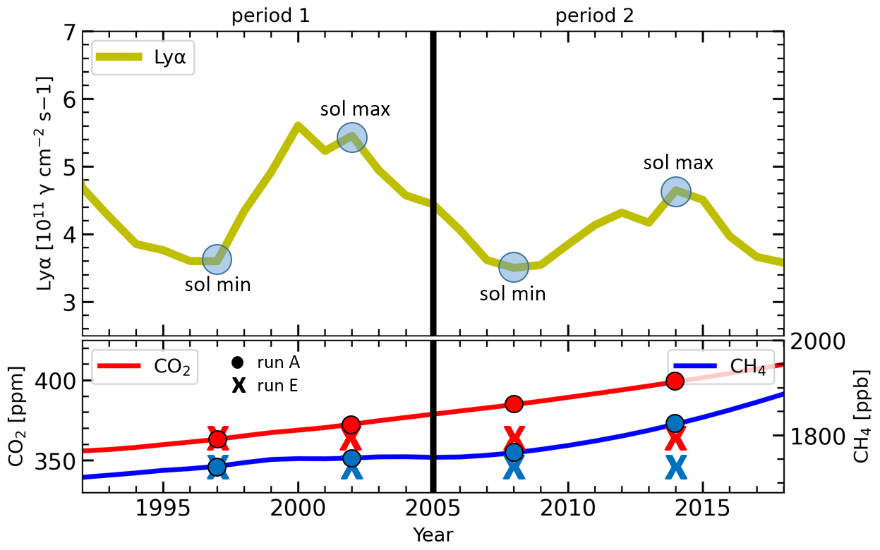
Figure 2 Time series of solar Lyα, CO₂, and CH₄ for 1992–2018. The corresponding Lyα, CO₂, and CH₄ values for the solar cycle maximum and minimum years used for this study are marked. The CO₂ and CH₄ values for run A are represented with dots, and for run E, they are represented with crosses. The study period is divided into period 1 as early (1992–2005) and period 2 as late (2005–2018).

3 Results and discussions

3.1 Solar cycle response in ice water content (IWC)

To determine whether the model agrees with satellite observations, we compared the ice water content (IWC) anomaly from the model with the satellite observations (see Fig. 3). IWC anomalies are calculated as follows:

$$\begin{array}{}\text{(1)}& {\mathrm{IWC}}_{\mathrm{anom}}=\mathrm{100}\mathit{\%}\cdot {\displaystyle \frac{\stackrel{\mathrm{‾}}{{\mathrm{IWC}}_{\mathrm{July}}}-\stackrel{\mathrm{‾}}{{\mathrm{IWC}}_{\mathrm{1981}-\mathrm{2018}}}}{\stackrel{\mathrm{‾}}{{\mathrm{IWC}}_{\mathrm{1981}-\mathrm{2018}}}}},\end{array}$$

where $\stackrel{\mathrm{‾}}{{\mathrm{IWC}}_{\mathrm{July}}}$ represent monthly zonal averages at 68^∘ N, and $\stackrel{\mathrm{‾}}{{\mathrm{IWC}}_{\mathrm{1981}-\mathrm{2018}}}$ are the averages of $\stackrel{\mathrm{‾}}{{\mathrm{IWC}}_{\mathrm{July}}}$ over the years 1981–2018. The IWC anomaly for satellite measurements are from the Solar Backscatter Ultraviolet (SBUV), Halogen Occultation Experiment (HALOE), Cloud Imaging and Particle Size (CIPS), and Solar Occultation For Ice Experiment (SOFIE) instruments. The time series of SBUV and HALOE data, as shown in Fig. 3, represent 3 years of sliding-averaged values. For more details on the satellite datasets, see Hervig et al. (2019). For this comparison, we used the MIMAS run A, in which the simulations are performed with increasing concentrations of CO₂ and CH₄. For the comparison, we applied the same calculation method to our model data as Hervig et al. (2019) did to satellite observations, namely, we used a threshold of 50 g km⁻³ for integrated water content because the polar mesospheric cloud (PMC) detection threshold for SBUV is 50 g km⁻³ (DeLand and Thomas, 2015, 2019).

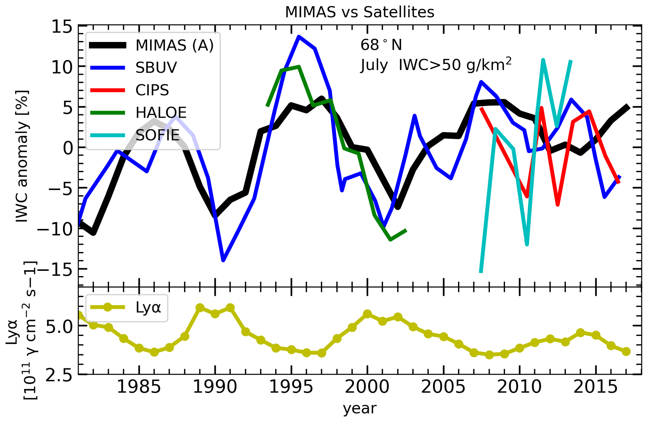
Figure 3 Time series of July mean IWC anomalies at 68^∘ N from model and satellites based on Hervig et al. (2019). Anomalies for each dataset are calculated as the difference from their long-term mean. To reduce year-to-year variability, the time series of SBUV and HALOE are smoothed using the sliding-average method of window size 3. Lyα–solar-cycle modulation is shown in the bottom panel.

We find an anti-correlation between MIMAS IWC anomaly and Lyα flux throughout the entire period (1981–2018), with a weaker response in the late period. In satellite observations, SBUV measurements also show an anti-correlation with Lyα flux until 2005, after which the response becomes weaker in agreement with MIMAS. The magnitude of the solar cycle IWC anomaly in SBUV and HALOE is of the same order as the IWC anomaly in MIMAS. The IWC anomalies of CIPS and SOFIE do not show a clear response to the solar cycle. We notice that the year-to-year IWC variation in CIPS and SOFIE is larger than the IWC modulation during a solar cycle.

IWC anomalies of SBUV and HALOE correlate well with MIMAS IWC anomalies before 2005 and progressively weaken afterwards. Lübken et al. (2009) found a good agreement between NLC parameters calculated by MIMAS and satellite observations. The general agreement between the main characteristics and trends of the ice layers in MIMAS and the observations suggests that the microphysical and photochemical processes in MIMAS cover the main processes relevant to NLC formation (Lübken et al., 2009).

3.2 Effect of NLC on water vapour (H₂O)

We calculated the zonal mean monthly averaged vertical profiles of H₂O and temperature to investigate the impact of NLC formation on the H₂O profile. Figure 4 shows the vertical H₂O profile averaged for July at 68^∘ N latitude and given at pressure altitudes $z_{\mathrm{p}}=H_{\mathrm{p}}\ln \left(p_{\mathrm{0}}/p\right)$, where p is the pressure of the model level, p₀ is the pressure at the surface, and H_p=7 km is the pressure scale height. This figure illustrates the effect of NLC formation on the background profile of water vapour since the H₂O profile with NLC differs from that without NLC. In the presence of NLC, there is a reduction in the water vapour mixing ratio (dehydration) between 83–90 km, i.e. in the region where the saturation ratio of water vapour is larger than 1. An enhancement in water vapour (hydration) is observed at altitudes between 79–83 km, where the saturation ratio of water vapour is smaller than 1. An environment with a water vapour saturation ratio larger than 1 is supersaturated, meaning ice particles can grow under these conditions, whereas a saturation ratio lower than 1 leads to ice sublimation. The degree of saturation depends on the background atmosphere's H₂O concentration and temperature. Ice particle formation starts at higher altitudes, where the temperature is the lowest, and then it sediments downward. During sedimentation, the ice particles grow by consuming H₂O from the surrounding background, which decreases background H₂O concentration. Then they approach a region with a saturation ratio smaller than 1, where they sublimate, releasing the water vapour. This is the so-called freeze-drying effect well discussed in a number of papers (Hervig et al., 2003; Lübken et al., 2009; Bardeen et al., 2010). The results in Fig. 4 illustrate the freeze-drying effect described above and also indicate that the effects of NLC on H₂O are not present below ∼ 79 km and above ∼ 97 km. This is the novelty of the results in Fig. 4. This is because the photochemical lifetime of water vapour below ∼ 79 km becomes larger than dynamical characteristic times, and distributions of water vapour become dynamically determined. Above 97 km, the saturation ratio of water vapour is smaller than 1; consequently, there is no NLC formation and consequently no effect on water vapour.

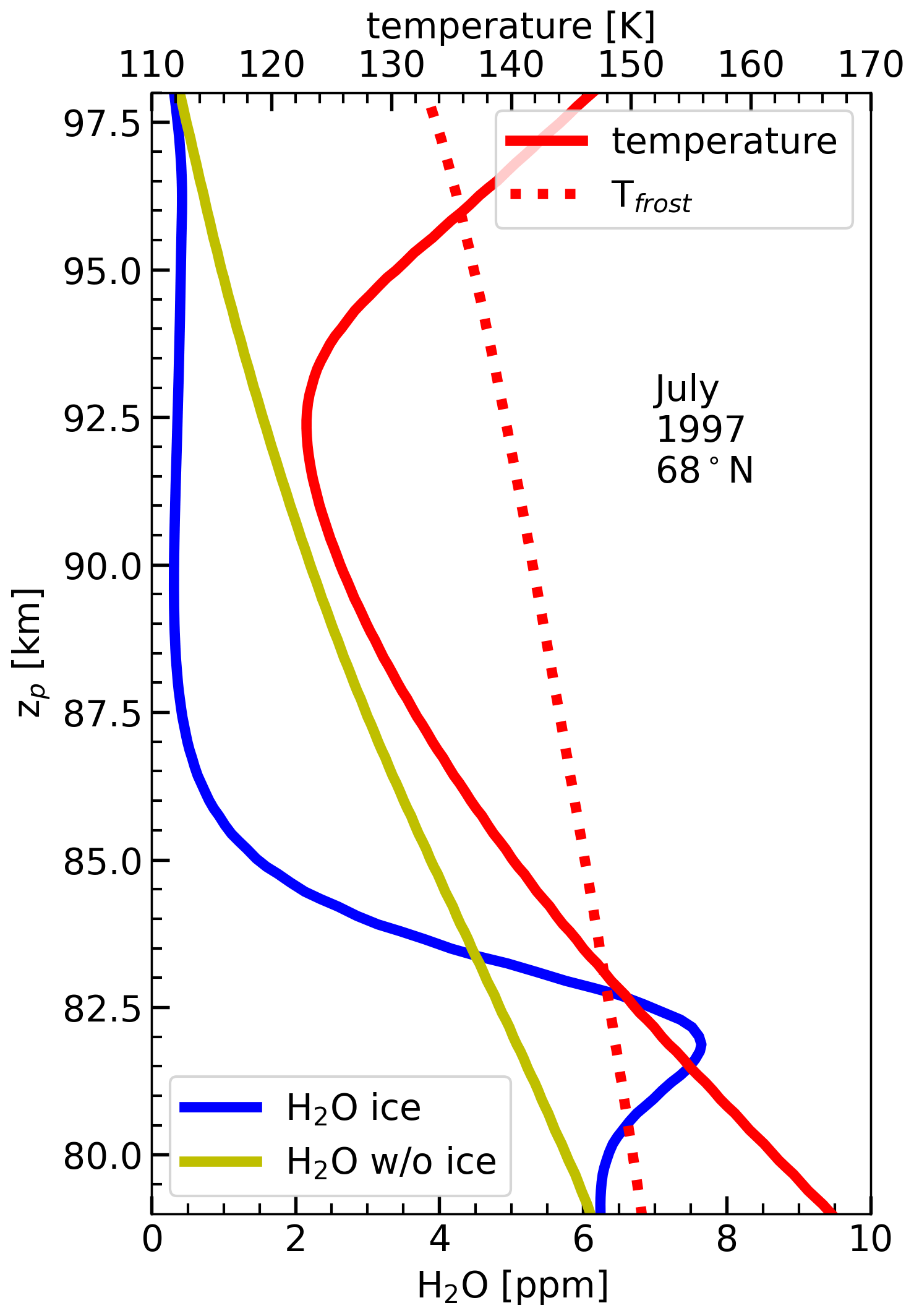
Figure 4 Zonally and monthly averaged H₂O and temperature profiles for July at 68^∘ N from MIMAS with and without NLCs. The doted red line represents frost point temperature. The blue lines show the background H₂O concentration with NLC, and the yellow lines show the H₂O concentration without NLC.

3.3 Effect of solar-cycle-induced temperature and photolysis changes on water vapour (H₂O)

We investigate the temperature change between the solar minimum (1997) and maximum (2002) due to solar irradiance variation and how these changes affect the H₂O profile. Different model runs performed for this study are summarized in Table 1. The differences (solar maximum − solar minimum) for H₂O and temperature profiles are shown in Fig. 5 for three model runs, namely E, F, and G. In run E, the solar-cycle-induced temperature change and photolysis influence H₂O concentration. In run F, only the temperature change caused by the solar cycle affects the H₂O concentration, while in run G, only the photolysis caused by the solar cycle affects the H₂O concentration (see Table 1). All of these runs are performed with constant CO₂ and CH₄ concentrations to avoid the effects of increasing GHG concentrations on temperature and H₂O profiles.

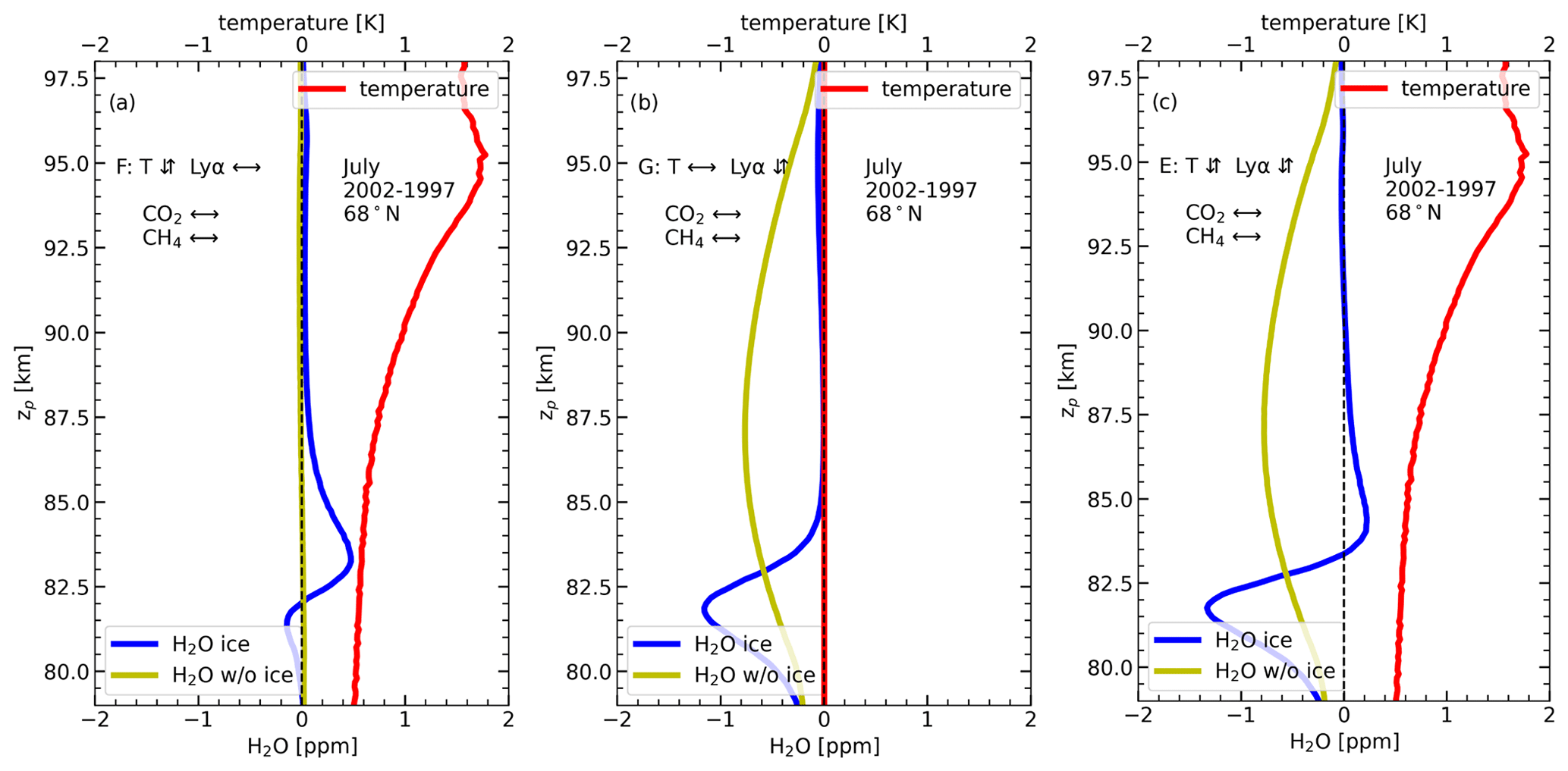
Figure 5 The difference in profiles between solar maximum (2002) and minimum (1997) for July mean H₂O and temperatures. The blue and yellow lines represent NLC and non-NLC conditions. In all cases, CO₂ and CH₄ values are constant, corresponding to 1997. (a) Run F: only temperature change effects on H₂O. (b) Run G: only photolysis change effect on H₂O. (c) Run E: both temperature change and photolysis change effects on H₂O.

In model run F, Lyα is held constant in MIMAS so the photolysis of H₂O is constant during the solar cycle. However, Lyα (and other bands) varies in the LIMA model so the background temperature varies with the solar cycle. Therefore, the change in the H₂O profile during the solar cycle is only due to the influence of the solar cycle on temperature and sequentially on microphysical processes. Figure 5a shows that the temperature increases during solar maximum compared to during solar minimum through the entire altitude range (79–97 km). The difference in temperature amounts to ∼ 0.5–1.7 K with maximum values at ∼ 95 km. During solar maximum, increased solar irradiance leads to greater absorption of solar radiation in the MLT region by molecular oxygen and water vapour, which heats the background atmosphere. Temperature differences decrease as altitude decreases because the intensity of solar radiation decreases due to atmospheric absorption by molecular oxygen and water vapour. The solar cycle effect in the H₂O profile with NLC (blue line) differs significantly from that without NLC (yellow line). Without NLC, the H₂O profile difference is nearly zero at all altitudes, indicating that the temperature changes do not significantly affect the background H₂O profile in the absence of NLC. With NLC, the H₂O profile difference is positive in the altitude range of 82–87 km and slightly negative in the range from 79–82 km. The atmosphere is warmer during solar maximum; therefore, the ice formation rate is lower during solar maximum. When the ice formation rate decreases, the amount of water vapour consumed from the background decreases; hence, more H₂O is left in the background during solar maximum compared to during solar minimum, resulting in a slightly positive response at NLC-forming altitudes above 83 km. Below that altitude, the slightly negative response is due to reduced ice formation in the nucleation region during solar maximum, which decreases H₂O released at ice sublimation altitudes. The positive difference peak at ∼ 83 km is located near the bottom of the H₂O-saturated zone. Ice formation and sublimation are more sensitive to an increase in background temperature in this zone (where the degree of saturation is close to 1) because, at these altitudes, the background temperature is almost equal to the frost point temperature so an increase in background temperature critically changes the degree of saturation. The change of the background temperature in a region where it is significantly lower than the frost point temperature is not critical for the degree of saturation. Overall, the temperature variation due to the solar cycle causes a positive H₂O response to the solar cycle at ice formation altitudes and a slightly negative response at ice sublimation altitudes.

In model run G (Fig. 5b), we consider only the effect of solar-cycle-induced Lyα variation on water vapour photolysis. The background temperature is held constant. Photolysis of H₂O by Lyα radiation molecules mainly produces atomic hydrogen (H) and hydroxyl (OH) in the upper atmosphere (∼ 90 %) and, to a lesser extent, O(¹D) with molecular hydrogen (∼ 10 %). The photolysis rate is higher during solar maximum due to the increased Lyα flux caused by the increased solar activity. Without NLC, the difference in the H₂O profile is negative at all altitudes (yellow line), indicating that the background H₂O is reduced during solar maximum due to increased photolysis. Figure 5b shows that the negative response peaks at an altitude of ∼ 87.5 km. The solar cycle effect on the photolysis of H₂O decreases above 87.5 km because the water vapour mixing ratio decreases with increasing altitude. The solar cycle variation of the photolysis effect decreases below 87.5 km because the solar Lyα radiation intensity decreases.

With NLC (blue line), the H₂O difference between the solar maximum and the solar minimum is essentially negative at ice sublimation altitudes (below ∼ 83 km) and negligible at higher altitudes (above ∼ 85 km). This is due to the redistribution of the H₂O profile during NLC formation (freeze drying). During solar maximum, the background H₂O concentration available for ice formation is reduced due to enhanced photolysis. The lower H₂O availability during solar maximum results in lower ice formation and, thus, lower H₂O release during sublimation, leading to lower hydration in the sublimation zone. For this reason, the solar cycle variation of the photolysis effect is more pronounced at sublimation altitudes. Above 85 km, the effect of photolysis, in the case with NLC, is minimal because of the lower availability of H₂O due to dehydration by NLC.

Figure 5c shows a combination of both effects, namely the solar-cycle-induced temperature change and photolysis effects on H₂O. Without NLC (yellow line), the H₂O profile shows a negative response at all altitudes, peaking at ∼ 87.5 km similar to run G (Fig. 5b, yellow line). We found that the variation of temperature has an almost negligible effect on the H₂O in the absence of NLC (see Fig. 5a, yellow line) so the negative response of water vapour without consideration of microphysical processes (yellow line on Fig. 5c) is mainly caused by the photolysis effect. With NLC (Fig. 5c, blue line), the combined effect of temperature and photolysis has a slightly positive response to water vapour in the ice formation zone (83–89 km) and a negative response in the ice sublimation zone (80–83 km). The slightly positive response is caused by the temperature modulation, and the negative response is primarily due to the photolysis modulation throughout the solar cycle.

The study proves that the water vapour response to the solar cycle is affected by the re-distribution of water in the presence of NLC. There may exist regions with positive correlations of water vapour with Lyα when NLC formation occurs. Without NLC, the water vapour always shows a negative correlation with the solar cycle. When comparing the effects of solar cycle modulations of temperatures and photolysis on H₂O, the photolysis has a stronger effect on water vapour; however, the variation of temperature induces a positive correlation of solar irradiance and H₂O.

4 Increasing greenhouse gases and reducing solar cycle

This section examines how the increase in GHGs affects the H₂O response to the solar cycle. To distinguish the GHG effects, we compared the model results with increasing CO₂ and CH₄ (run A) to the model run with constant CO₂ and CH₄ (run E). It is noted already that an increasing CO₂ concentration leads to a cooling of the middle atmosphere, and an increase in CH₄ concentration leads to an increase in H₂O concentration (see Sect. 2 for details). In Fig. 2, the concentrations of CO₂ and CH₄ increase during the late period, and at the same time, the peak of the Lyα flux decreases. In order to filter out the effect of reduced Lyα intensity, we calculated the H₂O response profile per unit of Lyα (ΔH₂O $/$ ΔLyα). Figure 6 shows the result for the first (1997–2002, blue line) and the second period (2008–2014, orange line) for model runs E (Fig. 6a) and A (Fig. 6b) respectively. These profiles show positive and negative responses depending on altitude. Under the conditions of constant GHGs (run E), the sensitivity of water vapour to Lyα does not change from the early to the late period (Fig. 6a). As expected, for the case of growing methane and carbon dioxide (run A), the sensitivity of water vapour to Lyα increases during the late period (orange line, Fig. 6b) compared to during the early period (blue line, Fig. 6b). This is because an increase in CO₂ (and consequently, a temperature decrease) leads to an intensification of microphysical processes and, hence, to the increased freeze drying. In addition, increasing methane leads to more water vapour in the upper mesosphere, which also leads to an increased water vapour variation with solar cycle.

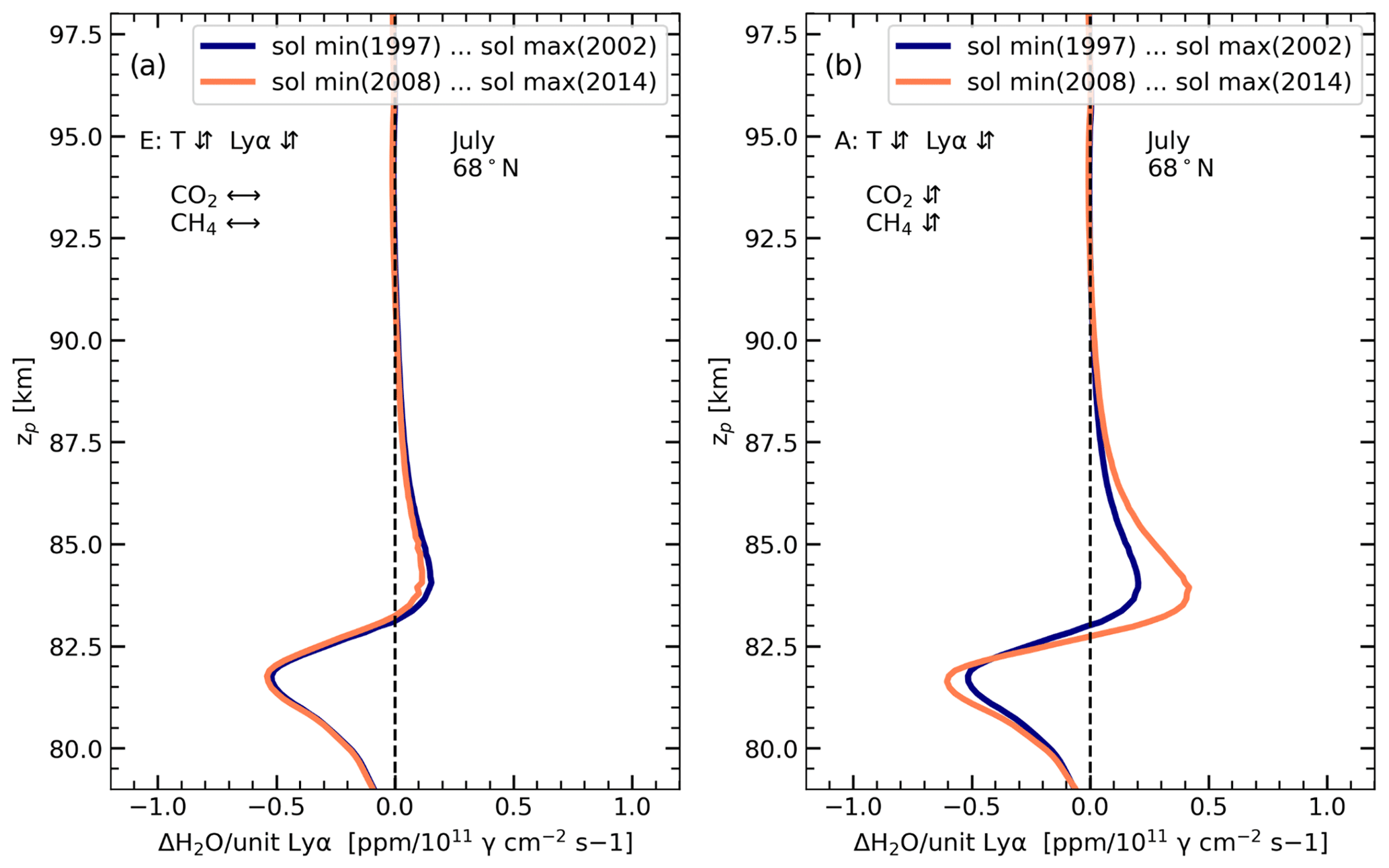
Figure 6 H₂O response per unit Lyα variations in July at 68^∘ N during the years between solar minimum and maximum in the early (1997–2002) and late (2008–2014) periods. (a) MIMAS model run E with constant CO₂ and CH₄. (b) MIMAS model run A with varying CO₂ and CH₄.

To study the effect of a decreasing Lyα amplitude during the late period (2008–2014), we calculated the ratio of water vapour absolute deviations between solar minimum and solar maximum for the early and late periods. The amplitude of Lyα variation is weaker during the late period (∼ 1.14×10¹¹ [phot. cm⁻² s⁻¹] per solar cycle) compared to the early period (∼ 1.85×10¹¹ [phot. cm⁻² s⁻¹] per solar cycle). The intensity of Lyα during the late-period solar maximum is reduced by ∼ 40 % compared to during the early period. As can be seen from Fig. 7a, the magnitudes of positive and negative H₂O responses decreased during the late period for model runs with constant GHGs (run E). In Fig. 6a, we found that the H₂O sensitivity to Lyα flux is the same in the early and late periods for the model run with constant GHGs (run E). Therefore, the reduced response of H₂O during the late period in model run E (Fig. 7a) is only due to the reduced solar Lyα variation. Comparing the late-period H₂O response to the solar cycle from model runs with constant GHGs (Fig. 7a, orange line) to that from model runs with increasing GHGs (Fig. 7b, orange line) suggests that both the positive and negative peak responses are enhanced by increasing GHG concentration. Due to the increased solar Lyα flux and greenhouse gases, the NLC and water vapour response are expected to increase during the current solar cycle 25 as the Lyα radiance has already exceeded the peak value of the previous solar cycle 24.

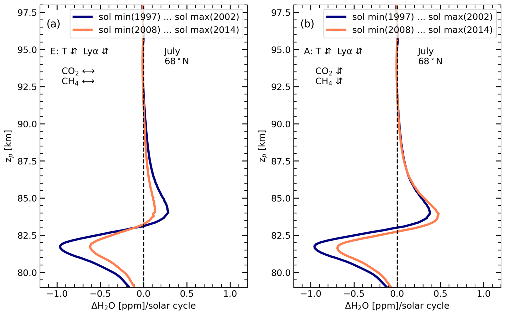
Figure 7 H₂O response to absolute solar cycle Lyα variations in July at 68^∘ N during the years between solar minimum and maximum in the early (1997–2002) and late (2008–2014) periods. (a) MIMAS model run E with constant CO₂ and CH₄. (b) MIMAS model run A with varying CO₂ and CH₄.

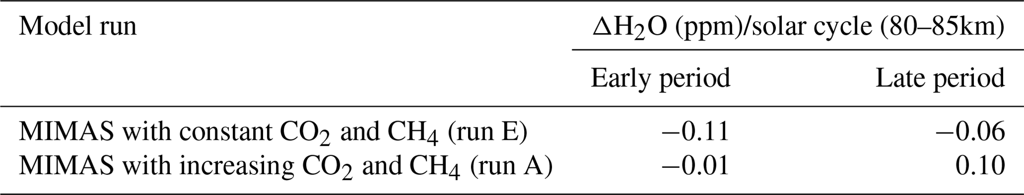
Table 2 The solar cycle H₂O response averaged over 80–85 km geometric altitude at 68^∘ N for model runs A and E.

5 Missing H₂O–solar-cycle response

A recent study by Hervig et al. (2019) reported a missing response in H₂O concentration to the solar cycle after 2005. In Fig. 8, we compare our model results of H₂O anomaly with the satellite observations. The H₂O response is averaged over the geometric altitudes of 80–85 km at 68^∘ N. For this comparison, we used MIMAS run A, where the increasing concentration of GHG is considered. The satellite observations are shown in Fig. 8 from HALOE, SOFIE, and MLS according to Hervig et al. (2019). HALOE shows a strong negative response to Lyα (−1.7 ppmv per solar cycle) during period 1, but in SOFIE and MLS, the response is almost absent (+0.2 ppmv per solar cycle) during period 2 (Hervig et al., 2019). For MIMAS, no clear H₂O–solar-cycle anti-correlation is noticed in the early period, but it was slightly positive in the late period, in agreement with SOFIE and MLS satellite observations. To investigate the H₂O response to Lyα variation in more detail, we analysed the vertical H₂O response profile at geometric altitudes similar to the satellite observations.

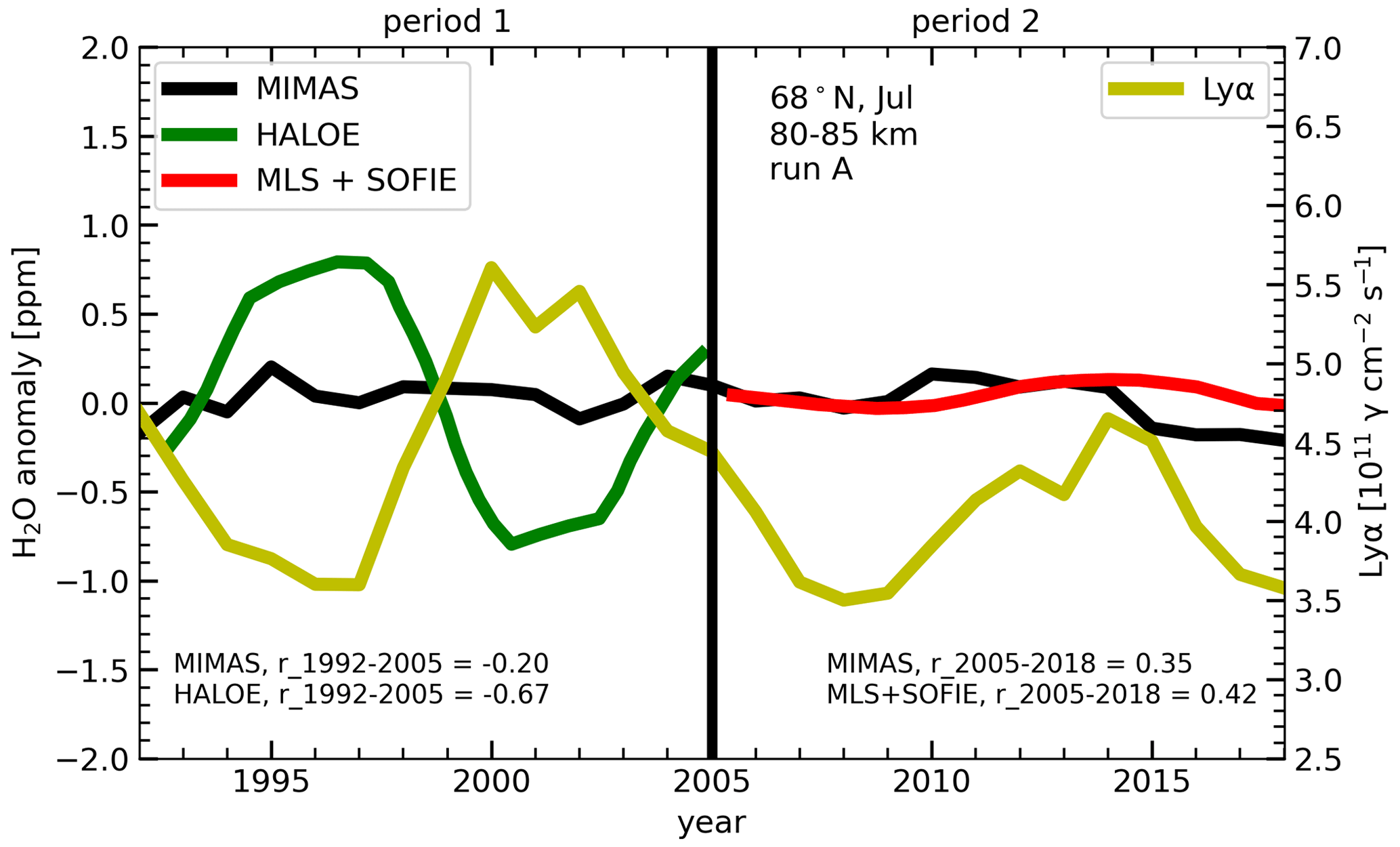
Figure 8 Time series of Lyα and H₂O anomalies as monthly averages for July at 68^∘ N for the altitude range of 80–85 km from MIMAS run A and satellites (HALOE and the composite data (MLS and SOFIE)). Satellite observations are according to Hervig et al. (2019). The H₂O–Lyα correlation is calculated for the early and late periods (see inlet).

Figure 9 shows the vertical profile of H₂O response in geometric altitudes for the model run with constant GHGs (run E, Fig. 9a) and growing GHGs (run A, Fig. 9b). The magnitude of the H₂O response at geometric altitudes (Fig. 9) differs from that at pressure altitudes (Fig. 7). This is because the geometric altitude of constant pressure levels is not constant and varies throughout the solar cycle but also with time due to increasing GHGs. Therefore, the magnitude of the H₂O response differs when converted from pressure altitudes to geometric altitudes.

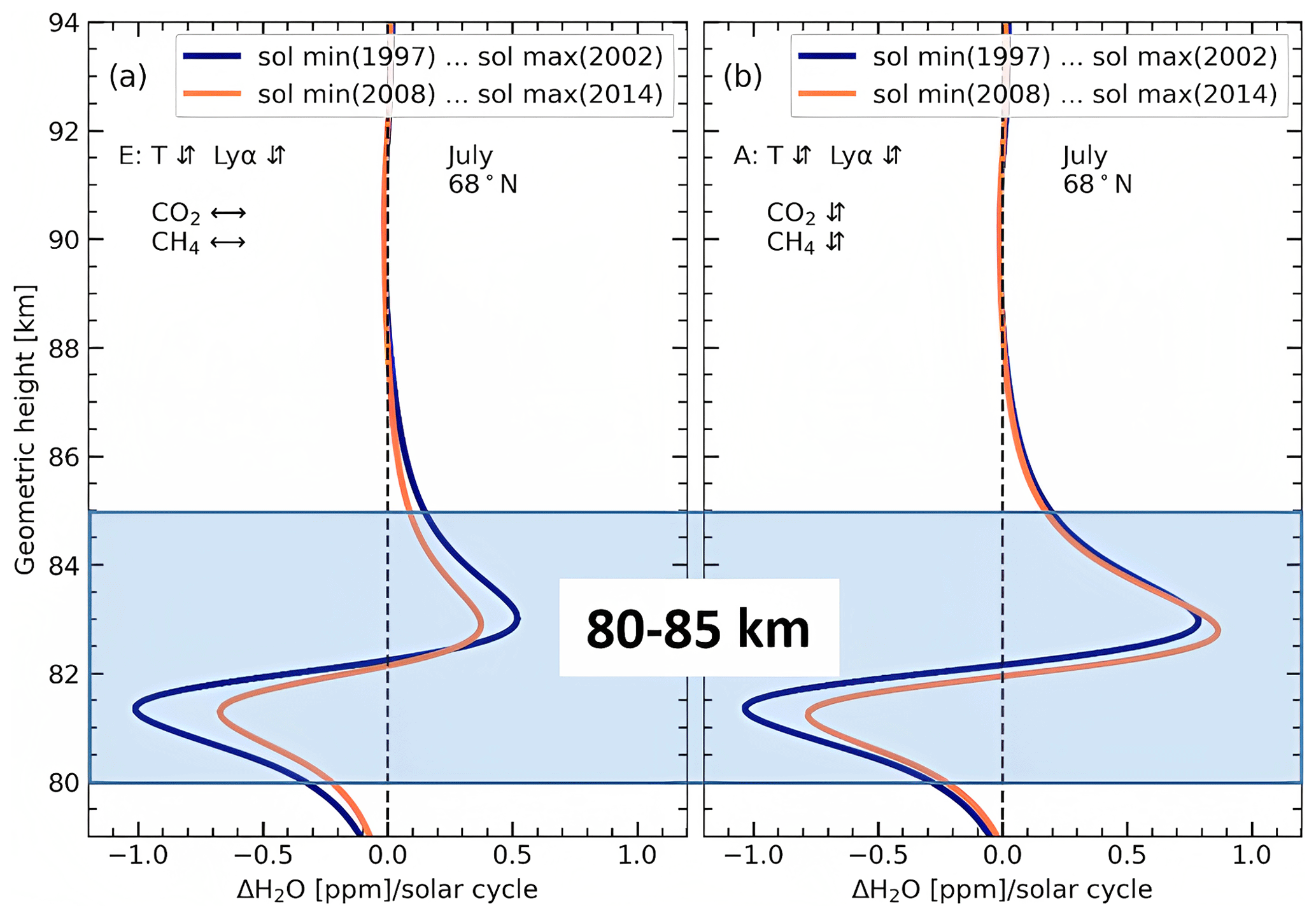
Figure 9 H₂O response to absolute solar cycle Lyα variations in July at 68^∘ N during the years between solar minimum and maximum in the early (1997–2002) and late (2008–2014) periods represented in geometric altitudes. The shaded region represents the altitude range used for calculating an average solar cycle response. (a) MIMAS model run E with constant CO₂ and CH₄. (b) MIMAS model run A with varying CO₂ and CH₄.

We focus on the 80–85 km geometric altitude range (Fig. 9, shaded region). There are positive and negative H₂O response zones within this altitude range, similarly to Fig. 7. We calculated the average H₂O response over the 80–85 km altitude range for MIMAS runs A and E, and this is given in Table 2. For the model run with growing GHGs (run A), the H₂O response averaged over an altitude range of 80–85 km changed from −0.01 ppm per solar cycle in the early period to 0.10 ppm per solar cycle in the late period (see Table 2). The H₂O response in the late period becomes slightly positive for run A, consistent with the satellite observations of SOFIE and MLS (see Fig. 8). The vertical profile of the H₂O–solar-cycle response clearly shows that H₂O response to the solar cycle is not completely missing in the late period. The missing response in the MIMAS H₂O, as shown in Fig. 8, occurred when averaging over the 80–85 km altitude range. Figure 9 demonstrates that the H₂O response shows nearly equal positive and negative responses within the 80–85 km altitude range (shaded region). Therefore, averaging the response in this altitude range becomes nearly zero as the positive and negative responses cancel out each other. When averaging over the altitude range of 80–82 km in the early period, we receive an H₂O response of −0.71 ppm per solar cycle and an anti-correlation between H₂O and Lyα. The results clearly shows that the small solar cycle response in MIMAS is a consequence of averaging over an altitude range of 80–85 km. It suggests that averaging H₂O response over an altitude range containing positive and negative responses may not provide a detailed understanding of the H₂O–solar-cycle response.

6 Conclusions

In this study, we used our ice particle model MIMAS along with the atmospheric dynamics model LIMA to investigate the response of H₂O to the solar cycle from 1992 to 2018. We investigated how NLC formation affects vertical H₂O profiles by running model simulations with and without microphysics. NLC formations are shown to redistribute H₂O profiles by consuming H₂O from the background at ice-forming altitudes (dehydration) and releasing it at ice-sublimating altitudes (hydration), which is known as the freeze-drying effect. To investigate the missing solar cycle response in satellite observations reported by Hervig et al. (2019), we divided the entire study period into an early period (1992–2005) and a late (2005–2018) period. We first investigated how the Lyα variation affects the H₂O profile between solar minimum and maximum in the early period. The solar Lyα variation affects the H₂O concentration at NLC altitudes mainly in two ways: through the effect of temperature change and through the effect of photolysis. To distinguish these two effects, we performed additional model simulations with different background conditions (see Table 1). We found that the modulation of water vapour, which comes through the temperature changes with the solar cycle, causes a slight positive H₂O response at ice-forming altitudes and a negative response at ice-sublimating altitudes. The solar cycle photolysis effect has only negative responses to the H₂O profile, and this response dominates at ice sublimation altitudes with NLC conditions. Our results for the case of photolysis effect only are supported by previous simulations, which also suggest that freeze drying significantly reduces the potential effect of Lyα photolysis on H₂O above 82 km, while the effect is enhanced at 80–82 km, where ice particles sublimate (von Zahn et al., 2004; Lübken et al., 2009).

To the best of our knowledge, we have for the first time identified a positive response of water vapour to Lyα variation in the MLT region, which is due to microphysical processes. It was assumed for a long time that water vapour only anti-correlates with the solar cycle at mesopause altitudes (e.g. Sonnemann and Grygalashvyly, 2005, and references therein). We should note that, in the Martian atmosphere where microphysical processes play a crucial role in water vapour distributions through the entire atmosphere in all seasons (e.g. Shaposhnikov et al., 2018), this effect may be important.

We have made a comparison between the model and satellite observations of the H₂O response to the solar cycle averaged over an altitude range of 80–85 km. The satellite observations from HALOE show a strong anti-correlation with the solar cycle in the early period, but the model shows a very small response in both the early and late periods. The vertical H₂O response profiles from MIMAS show that, within the 80–85 km altitude range, the positive and negative responses are almost equal in magnitude and symmetric. Therefore, averaging the response over this altitude range reduces the overall response in the model as positive and negative responses cancel each other out.

We also investigated the role of increasing GHGs in the H₂O–solar-cycle response. From the early to the late period, there are mainly two factors that affect the long-term H₂O solar cycle response: increasing CO₂ and CH₄ concentrations and the lower intensity of the solar cycle (see Fig. 2). We found that increasing GHG concentration increased the H₂O response to Lyα. The Lyα intensity during the late solar maximum decreased by 40 % compared to during the early solar maximum. Therefore, the overall response of H₂O to the solar cycle is also decreased in the late period. It should be noted that our results have limitations as they use constant dynamics for all years. We are looking forward to a new gravity-wave-resolving model for the investigation of the effects on changing dynamics due to changing GHGs and solar activity.