Fluid models capturing Farley–Buneman instabilities

It is generally accepted that modeling Farley–Buneman instabilities requires resolving ion Landau damping to reproduce experimentally observed features. Particle-in-cell (PIC) simulations have been able to reproduce most of these but at a computational cost that severely affects their scalability. This limitation hinders the study of non-local phenomena that require three dimensions or coupling with larger-scale processes. We argue that a form of the five-moment fluid system can recreate several qualitative aspects of Farley–Buneman dynamics such as density and phase speed saturation, wave turning, and heating. Unexpectedly, these features are still reproduced even without using artificial viscosity to capture Landau damping. Comparing the proposed fluid models and a PIC implementation shows good qualitative agreement.

1 Introduction

Magnetized Hall-drifting electrons in the E-region ionosphere induce polarization drifts on the unmagnetized ions which tend to overshoot electrostatic equilibrium and accumulate in the crests of the local density irregularities faster than diffusion opposes them (Sahr and Fejer, 1996). This mechanism, which results in the amplitude enhancement of local perturbations, is the Farley–Buneman instability. This phenomenon has been shown to modify the mean state of the ionosphere in various ways as well as the magnetosphere morphology by modifying the local conductivity through anomalous heating and nonlinear currents (Wiltberger et al., 2017).

Linear fluid theory of Farley–Buneman instabilities predicts some aspects of the dynamics reasonably well. Furthermore, linear kinetic theory shows that ion Landau damping effectively suppresses the growth of smaller wavelengths (Schmidt and Gary, 1973), which motivates the necessity of resolving kinetic ion effects. Nevertheless, the linear theory fails to explain several features observed in the experimental data obtained with rockets and coherent backscatter radars (Oppenheim et al., 1996; Sahr and Fejer, 1996). Although particle-in-cell (PIC) simulations have been able to model many aspects of the nonlinear physics of Farley–Buneman instabilities (Oppenheim et al., 2008; Oppenheim and Dimant, 2013; Young et al., 2020), their application to non-local scales has been very challenging due to the computational cost. This limitation has motivated the exploration of more cost-effective approaches like hybrid and fluid models, which often require much less computational resources because they do not resolve the velocity distribution of the plasma. For instance, Newman and Ott (1981) and Hassan et al. (2015) proposed a fully fluid dynamical system that models Landau damping with a viscosity term on the momentum equation that damps large wavenumbers. Because of the isothermal approximation, these simulations could not capture wave turning and other thermal effects (Dimant and Oppenheim, 2004).

This work describes a numerical framework based on the five-moment fluid model to simulate Farley–Buneman instabilities and assesses its capability for capturing nonlinear features reproduced previously with PIC simulations. First, we used the viscosity proposed by Hassan et al. (2015), including an energy equation for both species. The simulation parameters were similar to the ones used by Oppenheim et al. (2008) to compare our results with the PIC estimates. Then, we show that most characteristic nonlinear features can be reproduced even after removing the viscosity term from the five-moment system. These results are obtained even though the standard linear theory predicts that smaller structures will grow faster. Furthermore, we argue that the nonlinear signatures obtained without the viscosity are more similar to the correspondent PIC estimates. This last result suggests that the proposed fluid framework may dramatically increase the scalability of Farley–Buneman simulations.

2 A numerical framework for Farley–Buneman instabilities based on fluid equations

The Farley–Buneman instability is an electrostatic process with the dominant dynamics mostly restricted to a 2D plane perpendicular to B. Both the magnetized electrons and unmagnetized ions collide predominantly with neutral particles (Rojas and Hysell, 2021). Therefore, assuming both species are locally Maxwellian, the following five-moment fluid system should be capable of capturing most of the important physics (Schunk and Nagy, 2009):

$$\begin{array}{}\text{(1)}& {\displaystyle \frac{\partial n_{\text{s}}}{\partial t}}+\mathrm{\nabla }\cdot \left(n_{\text{s}}{v}_{\text{s}}\right)=\mathrm{0},\text{(2)}& {\displaystyle }\begin{array}{rl}{\displaystyle \frac{\partial v_{\text{s}}}{\partial t}}+& v_{\text{s}}\cdot \mathrm{\nabla }{v}_{\text{s}}={\displaystyle \frac{q_{\text{s}}}{m_{\text{s}}}}(E+v_{\text{s}}\times B)-{\displaystyle \frac{k{T}_{\text{s}}}{m_{\text{s}}}}\mathrm{\nabla }\ln n_{\text{s}}\\ -& {\displaystyle \frac{k}{m_{\text{s}}}}\mathrm{\nabla }{T}_{\text{s}}-{\mathit{\nu }}_{\text{sn}}{v}_{\text{s}}+R(T_{\mathrm{i}},v_{\mathrm{i}}),\end{array}\text{(3)}& {\displaystyle }\begin{array}{rl}{\displaystyle \frac{\partial T_{\text{s}}}{\partial t}}+& v_{\text{s}}\cdot \mathrm{\nabla }{T}_{\text{s}}+{\displaystyle \frac{\mathrm{2}}{\mathrm{3}}}{T}_{\text{s}}\mathrm{\nabla }\cdot v_{\text{s}}={\displaystyle \frac{\mathrm{2}{\mathit{\mu }}_{\text{sn}}}{\mathrm{3}k}}{\mathit{\nu }}_{\text{sn}}{v}_{\text{s}}^{\mathrm{2}}\\ -& {\mathit{\delta }}_{\text{sn}}{\mathit{\nu }}_{\text{sn}}(T_{\text{s}}-T_{\text{n}}),\end{array}\text{(4)}& {\displaystyle }{\mathrm{\nabla }}^{\mathrm{2}}\mathit{\varphi }=-{\displaystyle \frac{\mathrm{1}}{{\mathit{\epsilon }}_{\mathrm{0}}}}\sum _{\text{s}}{q}_{\text{s}}{n}_{\text{s}}.\end{array}$$

As usual, n_s, v_s, T_s, m_s, and q_s correspond to the density, velocity, temperature, mass, and charge of species s, respectively. The collision frequency between species s and neutral particles is represented by ν_sn, and μ_sn is the reduced mass of species s and the dominant neutral species. The frame of reference is moving with the neutral particles at a temperature T_n. On the right side of Eq. (3), the term on the left corresponds to collisional heating, while the one on the right captures collisional cooling. The term δ_sn captures the fraction of energy lost by particle s when it collides with a neutral (Dimant and Oppenheim, 2004). The electrostatic field was calculated by solving Poisson's Eq. (4).

The R(T_i,v_i) term on the right-hand side of Eq. (2) is a general regularization operator, and its purpose is to dampen the growth of larger wave numbers. Here, T_i and v_i are the ion temperature and velocity, respectively. Hassan et al. (2015) proposed a regularization term based on the ion viscosity operator but using the ion–neutral collision frequency instead of the Coulomb collision frequency. This term is used to damp large k modes and is only necessary for ion scales (Rojas et al., 2016). If we denote the stress tensor by Π, this regularizing viscosity has the form $R(T_{\mathrm{i}},v_{\mathrm{i}})=\mathrm{\nabla }\cdot \mathrm{\Pi }$, where

$$\begin{array}{}\text{(5)}& \mathrm{\Pi }=-{\displaystyle \frac{n_{\mathrm{i}}{T}_{\mathrm{i}}}{{\mathit{\nu }}_{\text{in}}}}\left(\mathrm{\nabla }{v}_{\mathrm{i}}+(\mathrm{\nabla }{v}_{\mathrm{i}}{)}^T-{\displaystyle \frac{\mathrm{2}}{\mathrm{3}}}\mathrm{\nabla }\cdot v_{\mathrm{i}}I\right).\end{array}$$

We used the operator proposed by Hassan et al. (2015) to model R(T_i,v_i) because it was successful in capturing several features of Farley–Buneman irregularities. Furthermore, the accuracy of this proxy will be assessed not by the quantitative estimates of the simulation but by whether it improves the resemblance to PIC simulations.

We chose a spectral solver to solve the five-moment system. Spectral methods are well-known to have outstanding accuracy and to scale very efficiently when periodic boundaries are applicable, and no shocks or discontinuities are expected (Hesthaven et al., 2007). These criteria are satisfied in the case of Farley–Buneman irregularities. We build the numerical solver using the Dedalus computational framework for solving general partial differential equations using sparse spectral methods (Burns et al., 2020). Our solver uses Fourier spatial discretizations with implicit integration of linear terms. The nonlinear terms are integrated explicitly with 3/2 padding for dealiasing. This solver was comprehensively described by Burns et al. (2020).

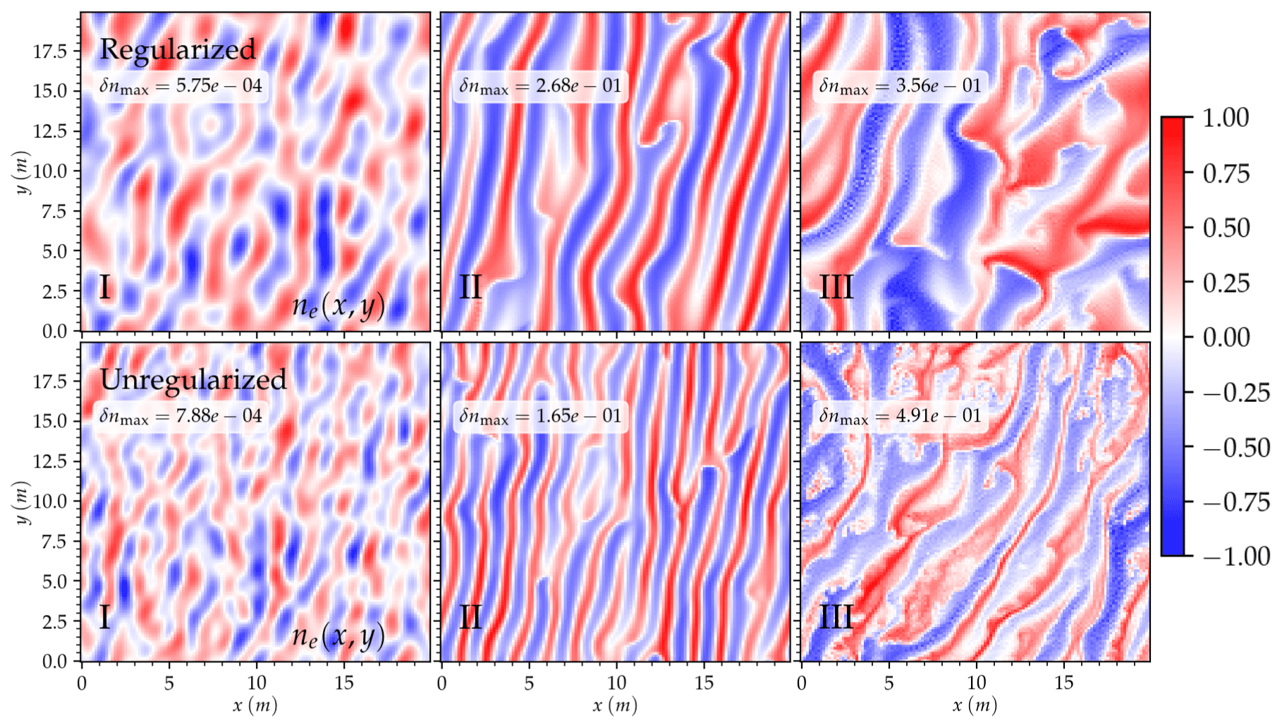
Figure 1 Electron density perturbation snapshot for both models. Here, δn_max indicates the maximum perturbation for that time instant. The color bar maps the corresponding fraction of δn_max. The top and bottom rows correspond to the regularized and unregularized models, respectively.

3 Simulation setup and results

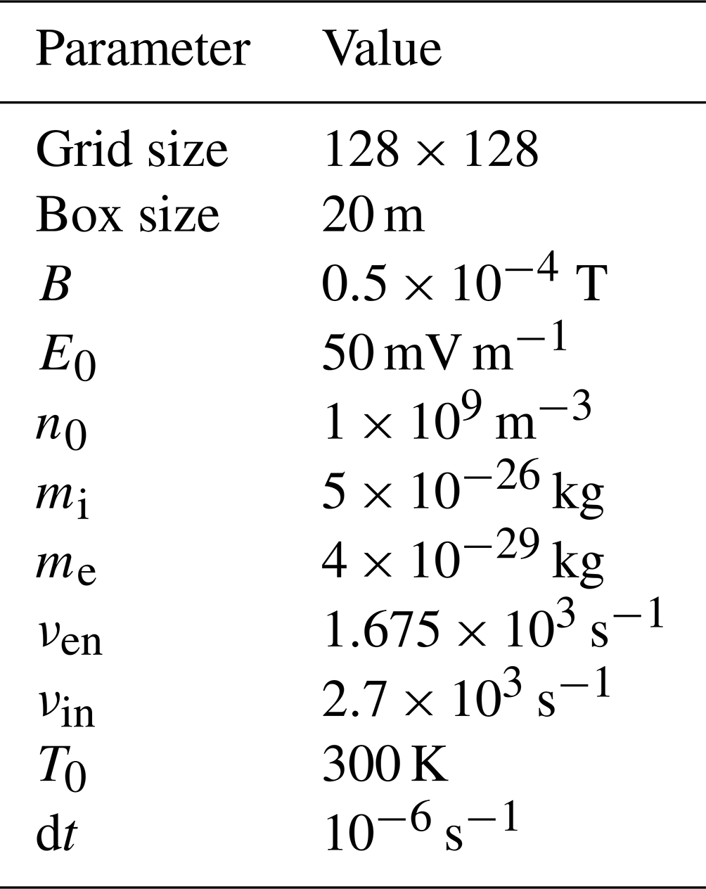
Some further simplifications can be applied to the five-moment system Eqs. (1)–(4). We omitted the gyro motion term from the ion momentum equation for the ions and used ${\mathit{\mu }}_{\text{in}}\approx m_{\mathrm{i}}/\mathrm{2}$ and δ_in=1. For the electrons, μ_en≈m_e, no regularization is included, and ${\mathit{\delta }}_{\text{en}}=\mathrm{3.5}\times {\mathrm{10}}^{\mathrm{4}}$ (Dimant and Oppenheim, 2004). Furthermore, we used the simulation parameters shown in Table 1. These parameters are the same as the ones used by Oppenheim et al. (2008) for their baseline simulation, except for the grid and box sizes, for which we used 8 times fewer grid points and half the box size, respectively. Notice that the electron mass m_e and the electron–neutral collision frequency ν_en have been artificially increased and reduced, respectively. Increasing the electron mass allows the use of larger time steps, but ν_en has to be reduced to maintain the same magnetization levels. The background electric and magnetic fields are defined in the $\widehat{y}$ and $\widehat{z}$ axes, respectively.

Table 1 Simulation parameters

The simulation box size is several times smaller than the largest ones used for recent purely kinetic (Oppenheim et al., 2008) and hybrid (Young et al., 2017, 2019) Farley–Buneman simulations. In this work, we will use small simulation boxes because we assume that most of the nonlinear features of the PIC simulations are independent of the dimensions of the simulation plane. Even though an energy cascade to larger wavelengths has been reported and it seems to be an issue of insufficiently large simulation boxes, we will not address this point in this work as we are interested in the growth rate of smaller scales. Furthermore, our claim about an improvement in scalability is based on the assumption that fluid models of few moments scale better than PIC kinetic simulations for the same accuracy when kinetic effects are not dominant.

We implemented two models. We will refer to the first as “regularized” and the second as “unregularized”. Both models will solve the continuity, momentum, energy, and Poisson equations, as shown in Eqs. (1–4). The only difference is that the regularized model includes the regularization operator described in Eq. (5) and the unregularized does not.

Figure 1 shows the electron density perturbation $n_{\text{e}}/n_{\mathrm{0}}-\mathrm{1}$ for both the regularized and the unregularized systems at representative times. Several features are common to both models. At linear regime I, we see dominant wave modes clearly. In the mixing regime II, most wave growth is aligned close to the E×B direction, and perpendicular secondary waves start to form. After saturation, in the turbulent regime III, we see a stable evolution of the electron density perturbation at around 20 % of the background density and density structures similar to the ones obtained with PIC simulations. Moreover, we see a slight turning of the waves in the direction consistent with linear theory, and it is assumed to be present in the nonlinear regime (Dimant and Oppenheim, 2004). On the other hand, the dominant wavelengths for the unregularized system are smaller (≈1.5 m, similar to the PIC simulation) than for the regularized case (≈2.5 m). This difference is consistent with the idea that the regularization term not only damps larger wave numbers but affects the dynamics of all the wave modes.

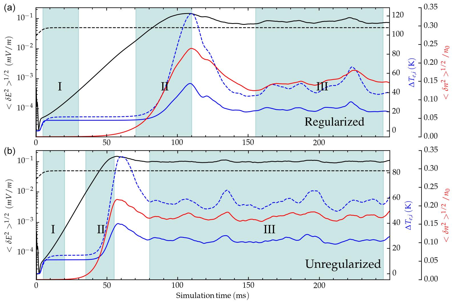
Figure 2 Time series for the electron temperature (blue dashed), ion temperature (blue), electron density averaged perturbation (red), background forcing field (black dashed), and root mean square of the electric field (black) for the regularized (a) and unregularized (b) models.

Although linear fluid theory predicts that smaller wavelengths will grow faster and destabilize the system without some form of regularization, we can see that the system not only remains stable but can capture several aspects of the expected nonlinear dynamics. This “self-regularization” may be a combination of several factors of numeric and physical origin. Even though spectral methods are well-known for having a minimal numerical diffusion compared to other approaches, this may play a minor role in damping the larger wave numbers. Other physical mechanisms which are captured in this model but not in some versions of the standard linear theory and which play a role in dampening smaller wavelengths are the stabilizing effect of a weak non-quasi-neutrality (Dimant and Oppenheim, 2011) and electron inertia (Hassan et al., 2015). An investigation of the extent of each of these mechanisms is beyond the scope of this paper and its topic of future work. Although the present simulations include the stabilizing effect of thermal dynamics, we have seen similar behavior using an isothermal system, namely, the presence of a dominant mode with no evidence of a growth rate proportional to k².

Standard metrics to diagnose the simulation, such as the root mean square (rms) of electron density, electric field perturbation, and the average heating, are presented in Fig. 2. The background electric field was raised from a value below the instability threshold at t=0 to the value shown in Table 1 in the first 2ms of the simulation. Both simulations show an increase in temperature due to Pedersen heating in the linear regime indicated as region I. All metrics reach saturation in the mixing regime characterized by region II and then stabilize in region III. The time series of both the regularized and, to a lesser extent, the unregularized simulations present an overshoot just before saturation. This behavior has been documented in hybrid (Rojas and Hysell, 2021) and fluid (Hassan et al., 2015) simulations, but it does not seem to be present in PIC simulations.

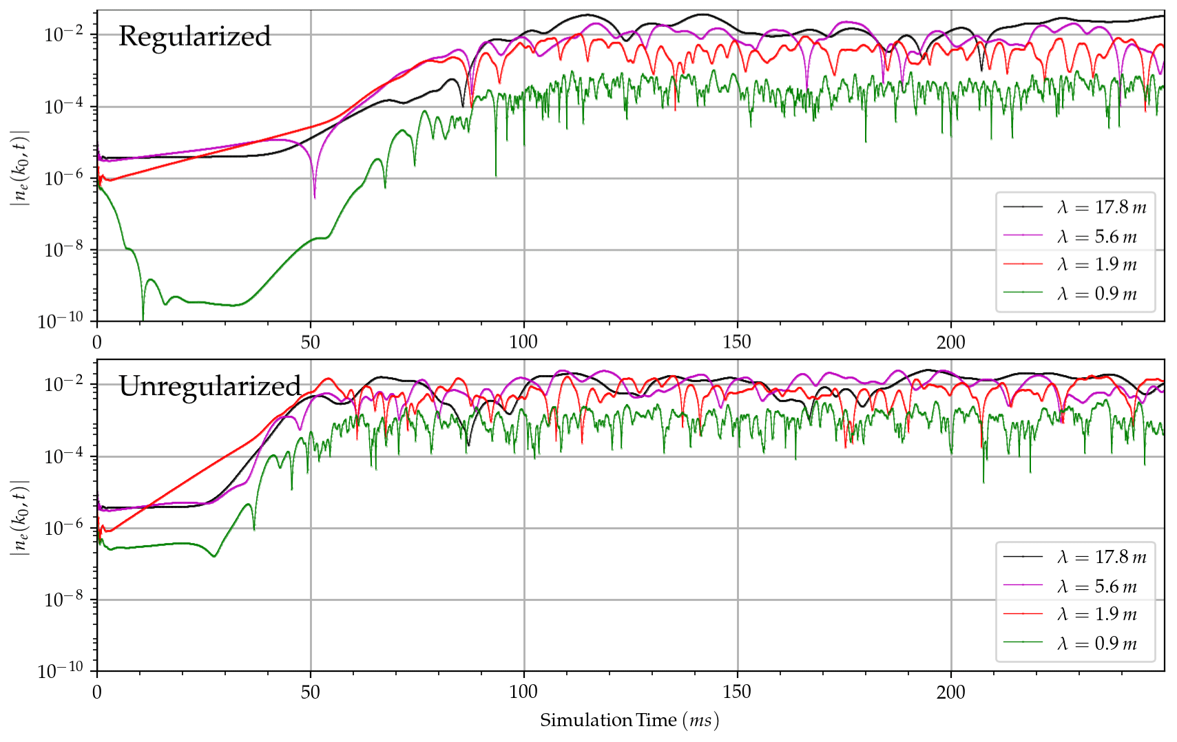
Figure 3 Time series of electron density perturbation spectral amplitude for specific wave numbers for both the regularized (a) and unregularized (b) systems.

In both simulations, the electron density and the perturbation electric rms field are larger than the corresponding PIC values. The fact that this difference is more considerable for the unregularized case (around twice the PIC metrics) suggests that the origin might be a lack of a proper damping mechanism. Although Oppenheim et al. (2008) also recovered a perturbation electric rms field larger than the background, the difference was smaller. They attributed this excess to factors like the truncation of smaller wavelengths (finite box size).

For instance, the rms field in physical space is the same as in Fourier space, so decreasing the amplitude of larger wave numbers would reduce the total rms. Moreover, the average ion temperature evolves similarly to kinetic simulations in both cases. Nevertheless, the mean electron heating is substantially lower, probably related to the simple temperature-independent collisional heating model used in both simulations. Even though there are several quantitative differences between these and the PIC results, it is interesting to notice that in the unregularized case, the saturation onset time is much closer to the corresponding time in the kinetic simulation (≈60 ms).

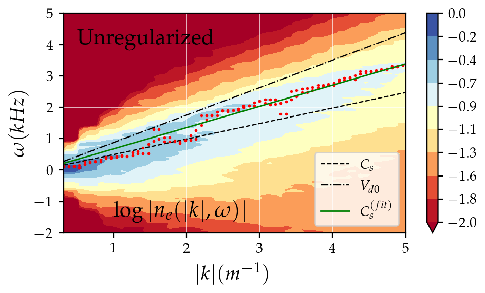
Figure 4 Electron density perturbation spectra versus wave numbers for the unregularized system. The red dots indicate the maximum amplitude for a particular k, and the green line represents the best fit of $k{C}_{\text{s}}^{\text{(fit)}}$ using anomalous γ_e,i as fitting parameters. V_d0 is the linear estimate of the phase speed using state parameters at the initialization.

Figure 3 illustrates the time series for the electron density perturbation for different wavelengths. Even though the regularized system shows strong damping for smaller wavelengths, both approaches seem to oscillate around similar amplitudes after saturation. This similarity may suggest that capturing the correct damping physics will affect the saturation onset time and the dominant wavelength value. Moreover, the amplitude of the larger wavelengths is comparatively larger for the regularized case.

The spectral properties of region III are summarized in Fig. 4 for the unregularized simulation. The spectral signatures of the regularized case are very similar but with smoother contours. The dominant wave modes propagate predominantly at phase speeds slightly above C_s. Heat capacity ratios representative of region III for both species can be estimated by fitting the expression for the ion-acoustic speed

$$\begin{array}{}\text{(6)}& C_{\text{s}}^{\text{(fit)}}=\sqrt{{\displaystyle \frac{{\mathit{\gamma }}_{\text{e}}\langle T_{\text{e}}{\rangle }_{\mathrm{III}}+{\mathit{\gamma }}_{\mathrm{i}}\langle T_{\mathrm{i}}{\rangle }_{\mathrm{III}}}{m_{\mathrm{i}}}}},\end{array}$$

to the most representative wave modes indicated by the red dots in Fig. 4. Here, 〈T_s〉_III indicates the average temperature of species s over region III. The ion's heat capacity ratio that produced the best fit with the simulated spectral peaks was γ_i≈2.62 in both models, which was smaller than the one reported in the corresponding PIC simulations by 14 %. On the other hand, the corresponding electron ratios were ${\mathit{\gamma }}_{\text{e}}^{\text{(r)}}\approx \mathrm{2.32}$ and ${\mathit{\gamma }}_{\text{e}}^{\text{(n)}}\approx \mathrm{2.29}$ for the regularized and unregularized cases, respectively. The obtained ratios for the electrons were larger than those obtained from PIC simulations by approximately 30 %. Nevertheless, this discrepancy was expected considering the oversimplification of the constant heating and cooling rates used for both species. This simplification is especially limiting for the electron thermal evolution, considering that electron heating associated with Farley–Buneman irregularities has been observed multiple times (Bahcivan, 2007).

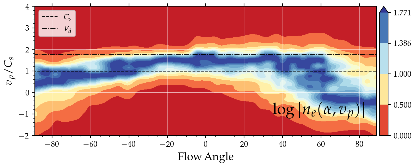
Figure 5 Spectra of electron density perturbations for $\left|k\right|=\mathrm{3}{m}^{-\mathrm{1}}$ with respect to phase speed and flow angle α for the unregularized system in region III. The spectra were normalized with the maximum power for each flow angle. V_d follows the definition of Fig. 4.

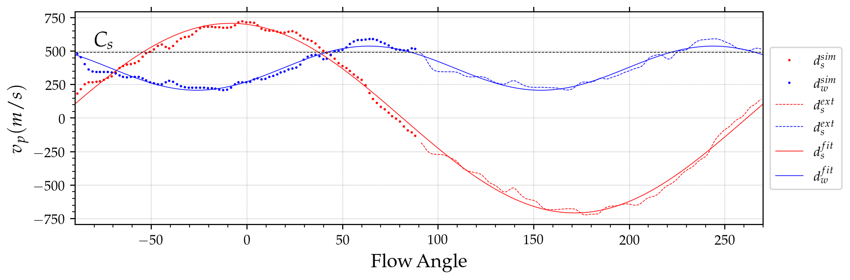
Figure 6 Simulated ($d_{\text{s,w}}^{\text{(sim)}}$), extended ($d_{\text{s,w}}^{\text{(ext)}}$), and fitted ($d_{\text{s,w}}^{\text{(fit)}}$) Doppler shift and spectral width calculated for regime III of the unregularized system. The dotted line indicates the local ion-acoustic speed.

The normalized spectra for $\left|k\right|=\mathrm{3}$ m⁻¹ are plotted in Fig. 5 with respect to the flow angle and the phase speed. Notice that the dominant modes have narrower widths and lie between the ion-acoustic and the convection speed. Both the Doppler shifts and the spectral widths can be calculated for each flow angle from these profiles. Considering that the system was assumed to be periodic, we can estimate the Doppler shifts and widths for the complete 360^∘ by rotating the simulated ones ($d_{\text{s,w}}^{\text{(sim)}}$) appropriately. The values estimated by this rotation are labeled as $d_{\text{s,w}}^{\text{(ext)}}$. These spectra were fitted to a modified version of a Doppler convection model used in Rojas et al. (2018):

$$\begin{array}{}\text{(7)}& {\displaystyle }{d}_{\text{s}}& {\displaystyle }=\left(a+{\displaystyle \frac{V_{\text{d}}^{\mathrm{2}}}{b}}\right)\cos (\mathit{\theta }+{\mathit{\theta }}_{\mathrm{0}}),\text{(8)}& {\displaystyle }{d}_w& {\displaystyle }=\mathit{\alpha }\left(a+{\displaystyle \frac{V_{\text{d}}^{\mathrm{2}}}{b}}\right)\sin \left(\mathrm{2}\right(\mathit{\theta }-\mathrm{2}{\mathit{\theta }}_{\mathrm{0}}\left)\right)+\mathit{\beta }.\end{array}$$

This empirical model relates Doppler shifts and widths to the flow angles θ. The local convection velocity V_d, wave turning angle θ₀, a, and b are fitting parameters. The red and blue lines in Fig. 6 correspond to the values of the model after estimating the parameters using a nonlinear optimization routine. We see that this empirical model agrees closely with the simulated values. Moreover, the fitted parameters are consistent with the experimental measurements by Nielsen and Schlegel (1985).

4 Conclusions

The results obtained with the proposed fluid models are consistent with the ones from PIC simulations in reproducing qualitative aspects of the Farley–Buneman instabilities. Moreover, using an unregularized five-moment fluid system, we could still reproduce most of the qualitative aspects of the diagnostics obtained with PIC simulations despite the predictions of standard linear theory. To our knowledge, this is the first time a fully fluid model is able to achieve this. Furthermore, the stabilization mechanisms of the proposed fluid electrostatic model seem to avoid the growth rates γ∝k². These results suggest that we may have to reconsider the necessity for capturing ion Landau damping accurately.

Even though the simulation box sizes used in this work are small compared to the dimensions used in recent PIC simulations, the potential of scalability relies on the fact that if kinetic effects are not dominant, fluid simulations usually require much less computational resources than PIC implementations to achieve similar accuracy.

Several interesting questions were raised: what nonlinear damping processes modulate the dominant wavelengths and onset saturation time? Would it be possible to build a Landau fluid proxy that captures enough of the physics we have access to by coherent backscatter radars? Would it be possible to modify the proposed fluid system to improve its scalability? Could these results be limited to spectral solvers? We will try to answer these questions in future studies.

Furthermore, we think this has significant implications for the plasma and space physics communities because it may open the door to other researchers having fluid plasma models to explore this topic.