Effect of intermittent structures on the spectral index of the magnetic field in the slow solar wind

Intermittent structures are ubiquitous in the solar wind turbulence, and they can significantly affect the power spectral index (which reflects the cascading process of the turbulence) of magnetic field fluctuations. However, to date, an analytical relationship between the intermittency level and the magnetic spectral index has not been shown. Here, we present the continuous variation in the magnetic spectral index in the inertial range as a function of the intermittency level. Using the measurements from the Wind spacecraft, we find 42 272 intervals with different levels of intermittency and with a duration of 5–6 min from 46 slow-wind streams between 2005 and 2013. Among them, each of the intermittent intervals is composed of one dominant intermittent structure and background turbulent fluctuations. For each interval, a magnetic spectral index α_B is determined for the Fourier spectrum of the magnetic field fluctuations in the inertial range between 0.01 and 0.3 Hz. A parameter I_max, which corresponds to the maximum of the trace of the partial variance increments of the intermittent structure, is introduced as an indicator of the intermittency level. Our statistical result shows that, as I_max increases from 0 to 20, the magnetic spectrum becomes gradually steeper and the magnetic spectral index α_B decreases from −1.63 to −2.01. Accordingly, for the first time, an empirical relation is established between α_B and I_max: ${\mathit{\alpha }}_B=\mathrm{0.4}\exp (-I_{\max }/\mathrm{5})-\mathrm{2.02}$. The result will help us to uncover more details about the contributions of the intermittent structures to the magnetic power spectra and, furthermore, about the physical nature of the energy cascade taking place in the solar wind. It will also help to improve turbulence theories that contain intermittent structures.

1 Introduction

Intermittent structures are ubiquitous in the solar wind turbulence. They correspond to the long tail of the non-Gaussian probability distribution functions of plasma or field fluctuations (Burlaga, 1991b; Marsch and Tu, 1994, 1997). Previous studies have revealed that intermittent structures are associated with current sheets and different types of discontinuities at small scales (tens of seconds) (Burlaga, 1969; Veltri and Mangeney, 1999; Servidio et al., 2012; Wang et al., 2013; Osman et al., 2014) as well as with the boundary between two adjacent flux ropes at large scales (tens of minutes) (Bruno et al., 2001; Borovsky, 2008) in the solar wind turbulence. These structures play an important role in the turbulence cascading and dissipation processes (Tu and Marsch, 1995; Bruno and Carbone, 2013; and the references therein).

Intermittent structures with large-amplitude fluctuations make a substantial contribution to the shape and power level of magnetic field spectra, which are directly related to the physical nature of the energy cascade taking place in the solar wind (Sari and Ness, 1969; Salem et al., 2007; Li et al., 2011; Borovsky, 2010). They often make the magnetic spectra become steeper (Siscoe et al., 1968; Burlaga, 1968; Salem et al., 2009). In previous studies, time series of discontinuities have been reported to produce an f⁻² energy spectrum (Sari and Ness, 1969; Roberts and Goldstein, 1987; Champeney, 1973; Dallas and Alexakis, 2013) in the inertial range. Moreover, more recently, it has been found that the discontinuities can also produce magnetic power spectra that are shallower than f⁻². Li et al. (2011) studied the effect of current sheets on the magnetic power spectrum from Ulysses observations. They found that the abundant-current-sheet periods and current-sheet-free periods show $f^{-\mathrm{5}/\mathrm{3}}$ Kolmogorov scaling and $f^{-\mathrm{3}/\mathrm{2}}$ Iroshnikov–Kraichnan scaling, respectively. Accordingly, they proposed that the current sheet is the cause of the Kolmogorov scaling. This finding was confirmed by Borovsky (2010), who created an artificial time series that preserves the timing and amplitudes of the discontinuities from Advanced Composition Explorer (ACE) spacecraft observations. The artificial time series produces a magnetic power-law spectrum with a slope near the Kolmogorov $f^{-\mathrm{5}/\mathrm{3}}$ scaling in the inertial range. They emphasize that any interpretation of the dynamics or evolution of the solar wind turbulence should account for the contribution of strong discontinuities in the measurements. Intermittent structures can also lead to anomalous (multifractal) scaling of structure functions (Veltri and Mangeney, 1999; Veltri, 1999; Salem et al., 2007, 2009).

Intermittent structures also influence the magnetic spectral anisotropy of fluctuations in the solar wind turbulence. The magnetic spectral index of magnetic field fluctuations has been reported to be anisotropic with respect to the scale-dependent local mean field in the inertial range (Horbury et al., 2008; Podesta, 2009; Luo and Wu, 2010; Chen et al., 2011; Forman et al., 2011; Wicks et al., 2011). After removing the intermittency from the turbulence, Wang et al. (2014) found that the anisotropy of the magnetic spectral index nearly disappeared. The magnetic spectrum in the parallel direction becomes shallower from f⁻² to $f^{-\mathrm{5}/\mathrm{3}}$, which is close to the scaling in the perpendicular direction. They concluded that the observed magnetic spectral anisotropy could result from intermittency. This result was confirmed by Telloni et al. (2019). Wang et al. (2015) made a comparison between the spectral anisotropy of magnetic fluctuations with low amplitude and those with moderate amplitude. The statistical results showed that anisotropy is only present in the moderate-amplitude situation, whereas it is absent in the low-amplitude cases. Accordingly, they suggested that magnetic spectral anisotropy is dependent on the fluctuation amplitude. Later, Wu et al. (2020) presented an analysis on the scaling anisotropy with a stationary background field and found the same isotropy for the moderate-amplitude fluctuations after removing those intermittent structures. Using numerical simulation in 3D magnetohydrodynamic turbulence, Yang et al. (2017) found the influence of intermittency on the quasi-perpendicular scaling of magnetic field and velocity fluctuations.

Recently, the magnitude and thickness of current sheets have also been found to have a significant effect on the power level in the dissipation range and the frequency location of the magnetic spectral break (Borovsky and Podesta, 2015; Borovsky and Burkholder, 2020; Podesta and Borovsky, 2016). Researchers have also studied the heating effect of the intermittent structures using both observations (Osman et al., 2011, 2012b, a; Borovsky and Denton, 2011; Wang et al., 2013; Liu et al., 2019; Zhou et al., 2022) and simulations (Parashar et al., 2009; Servidio et al., 2012; Wan et al., 2012; Zhang et al., 2015).

From the previous studies mentioned above, people have realized that the intermittent structure is an important part of the solar wind turbulence, and it can significantly affect the shape and power level of the magnetic power spectrum. A close correspondence between intermittency and changes in the second-order scaling properties has been well established. There is a huge amount of literature on the correction of the scaling properties due to intermittency, and many improved cascade models have been proposed to revise the original Kolmogorov results. However, to date, no analytical relationship between the magnetic spectral index and the level of intermittency has been shown. The main novelty of this work is that we show, for the first time, the analytical relationship between the magnetic spectral index and the level of intermittency by performing a fit on the observational results. Here, we will present the continuous variation in the magnetic spectral index as a function of the intermittency level, using measurements from the Wind spacecraft taken in the slow solar wind between 2005 and 2013. More than 42 000 intervals with different levels of the intermittency are selected from 46 slow-wind streams. Our result shows that the magnetic power spectrum between 0.01 and 0.3 Hz in the inertial range gets steeper from −1.63 to −2.01 as the intermittency level increases from 0 to 20. This will help us to gain more detailed information with respect to the effect of intermittency on the turbulence cascading process and will also supply an empirical relation for the theoretical and numerical studies in the future.

The paper is organized as follows: Sect. 2 introduces the data used in this work and the methods applied to find the intermittent structures and to determine both the intermittency level and the spectral index of magnetic fluctuations in the inertial range; Sect. 3 shows our observations, including cases and statistical results; Sect. 4 discusses the consequences of our results as well as the influence of magnetic compressibility and anisotropy on the results; and Sect. 5 provides a summary of this work.

2 Data and methods

We use magnetic field and plasma data measurements, both with a time resolution of Δt=3 s, obtained by magnetic field investigation (Lepping et al., 1995) and a 3D plasma analyzer (3DP; Lin et al., 1995), respectively, aboard the Wind spacecraft between 2005 and 2013. During this period, the Wind spacecraft was located at the Lagrangian point L1. Here, we focus on the slow-wind streams with a proton bulk velocity of V_SW≤450 km s⁻¹, and data observed within the compression regions that are followed immediately by fast-wind streams are discarded. The compression region is much more complicated and dynamic than the typical slow wind of interest, and it is outside the scope of this work. The plasma data are used here to get the bulk velocity for data selection and to get the proton number density in order to convert the magnetic data into Alfvén units. In addition, the plasma data are also used to calculate Alfvénicity for the purpose of revealing the nature of intermittent structures.

From the 8-year observations, we find 46 slow-wind streams. Each of the stream lasts about 2–5 d. Figure 1 shows one of the selected slow-wind streams observed from 12:00:00 UT on 5 December 2007 to 00:00:00 UT on 9 December 2007. Figure 1a, b, and c are the time variations in the magnetic field (black) and proton velocity (blue) vectors in geocentric solar ecliptic (GSE) coordinates. Figure 1d shows the magnitude of the magnetic field. During the 3.5 d interval, the absolute value of the x component of the proton velocity shown in Fig. 1a decreases from ∼ 360 to ∼ 300 km s⁻¹. Therefore, this interval is out of the compression region and is not adjacent to fast wind.

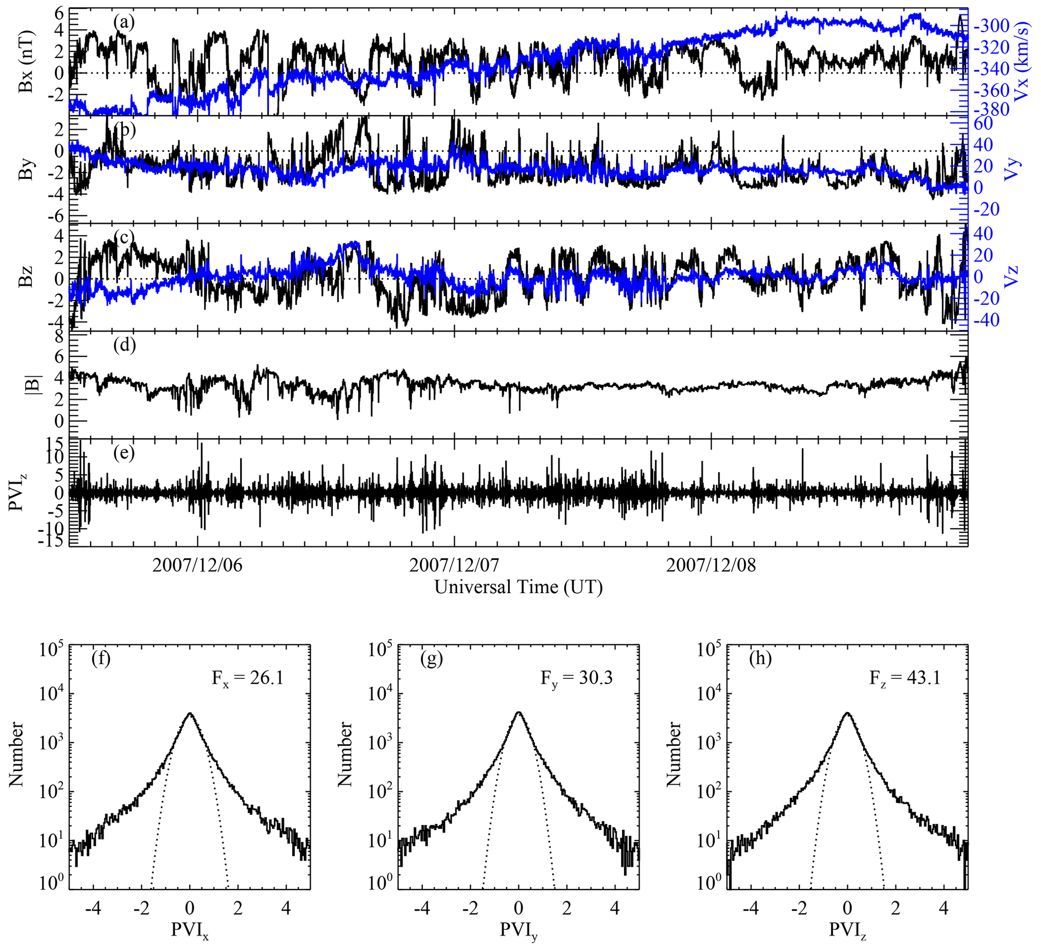
Figure 1 A typical slow-wind stream observed from 12:00:00 UT on 5 December 2007 to 00:00:00 UT on 9 December 2007 by the Wind spacecraft at the L1 point. (a–c) Time variations in the three components of the magnetic field vector (black) and proton velocity vector (blue) in the GSE coordinates. Horizontal dotted lines correspond to 0 nT. (d) Magnetic field magnitude. (e) Normalized partial variance of increments (PVI) for the z component of the magnetic field vector at the timescale of τ=24 s. (f–h) Probability distribution function (PDF, solid black curves) of the PVI for the three respective components of magnetic field. The flatness F_i ($i=x,y,z$) of each distribution is marked in each panel. Dotted curves denote the standard Gaussian distribution.

A parameter named normalized partial variance of increments (PVI) is applied to quantitatively analyze the intermittency in the solar wind turbulence, following previous studies (Marsch and Tu, 1994; Greco et al., 2008; Osman et al., 2011; Wang et al., 2013). For a component of the magnetic field vector in a given slow-wind stream, the time series of the PVI is presented as follows:

$$\begin{array}{}\text{(1)}& {\mathrm{PVI}}_i(t,\mathit{\tau })={\displaystyle \frac{\mathit{\delta }{B}_i(t,\mathit{\tau })}{\sqrt{<{\left|\mathit{\delta }{B}_i(t,\mathit{\tau })\right|}^{\mathrm{2}}>}}},\end{array}$$

where B_i(t) is the time series of the i component of the magnetic field vector ($i=x,y,z$), $\mathit{\delta }{B}_i\left(t\right)=B_i(t+\mathit{\tau })-B_i\left(t\right)$, and $<\mathrm{\dots }>$ denotes an ensemble average in the given stream. The time lag τ is selected as 24 s following Wang et al. (2013), corresponding to a spatial separation within the inertial range. In the following, we will refer to the PVI_i(t,τ) as PVI_i(t) for simplicity without further specification. Figure 1e shows the time series of PVI_z(t) for the stream. Many spikes appear in the time series of PVI_z(t), which correspond to large-amplitude fluctuations embedded in the background turbulence.

In Fig. 1f, g, and h, we demonstrate the probability distribution function (PDF, solid black curves) of the PVI for the three respective components of the magnetic field. The dotted curves are a standard Gaussian distribution, and they are plotted for easy comparison. The Gaussian distributions are located between the PVI range [$-\mathrm{2},\mathrm{2}$]. Beyond this range, the observed distribution curves exhibit long tails, and the tails extend even beyond the plotted range [$-\mathrm{5},\mathrm{5}$]. The PVI range [$-\mathrm{2},\mathrm{2}$] will then be used to select intermittent structures. Actually PVI_z can achieve ±10, as shown in Fig. 1e. Thus, it is clear that the profiles of the PDF for the three components (PVI_x, PVI_y, and PVI_z) all deviate significantly from the Gaussian distribution and have long tails when the absolute value of the PVI_i increases. The long tails of the non-Gaussian PDF profiles indicate the existence of intermittent structures.

We calculate the flatness for each distribution as follows: $F_i=<\left({\mathrm{PVI}}_i\right(t){)}^{\mathrm{4}}>/<({\mathrm{PVI}}_i\left(t\right){)}^{\mathrm{2}}{>}^{\mathrm{2}}$, where $<\mathrm{\dots }>$ still denotes the ensemble average in the given stream. An empirical rule is that the minimum number N of data points in the time series to be used to accurately calculate moments of order M is $N={\mathrm{10}}^{M+\mathrm{1}}$ (see, e.g., Dudok de Wit, 2004). In the case shown in Fig. 1, the total number of samples is 100 800. As flatness (the fourth-order moment) is considered here, the total number of samples meets the requirement, which is larger than the minimum number N=10⁵. The flatness values are marked as F_x=26.1, F_y=30.3, and F_z=43.1 in Fig. 1f, g, and h, respectively. They are much larger than 3 (characteristic of a standard Gaussian distribution). This again indicates that the fluctuations are highly intermittent.

The criterion $\left|{\mathit{PVI}}_i\right(t\left)\right|>\mathrm{2}$ is applied for the basic identification of intermittent structures. First, we find the time instants that satisfy at least one of the following conditions: $\left|{\mathrm{PVI}}_x\right(t\left)\right|>\mathrm{2}$, $\left|{\mathrm{PVI}}_y\right(t\left)\right|>\mathrm{2}$, or $\left|{\mathrm{PVI}}_z\right(t\left)\right|>\mathrm{2}$. Some of the instants are isolated, whereas some of them are clustered and continuous. Structures are only chosen for the following study if the number of continuous instants is not smaller than 3. The remaining instants are ignored. A continuous series of intermittent instants is considered to be an intermittent structure. Moreover, if the number of instants between two adjacent structures is smaller than 3, the two structures and the data points between them are merged together and are seen as one “long-lived” structure. For a given structure, we use t_B and t_E to denote its beginning time and ending time, respectively, and we use $(t_{\mathrm{E}}-t_{\mathrm{B}})/\mathrm{\Delta }t$ as the width of the structure in the unit of data points. An interval between [t_B−150 s, t_E+150 s] is called an intermittent interval. After the 10 % data gap constraint is applied, we find 56 398 intermittent intervals from 46 slow-wind streams between 2005 and 2013.

Figure 2 shows a typical case of an intermittent interval observed by the Wind spacecraft on 23 February 2007. Figure 2a, b, and c present the time variations in the three components of the magnetic field vector (black) and the proton velocity vector (gray). The magnetic field data are transformed into Alfvén units (i.e., $B/\sqrt{{\mathit{\mu }}_{\mathrm{0}}{m}_{\mathrm{p}}〈n_{\mathrm{p}}〉}$, where μ₀ is susceptibility, m_p is proton mass, and 〈n_p〉 is the average proton number density of the ∼ 5 min interval), so that the fluctuation amplitudes of the magnetic field and the velocity are comparable. Figure 2d shows the time variations in the magnetic field magnitude. Figure 2e shows the time series of the PVI_x(t) (purple), PVI_y(t) (yellow), and PVI_z(t) (green) as well as the trace PVI ($I=\sqrt{({\mathrm{PVI}}_x{)}^{\mathrm{2}}+({\mathrm{PVI}}_y{)}^{\mathrm{2}}+({\mathrm{PVI}}_z{)}^{\mathrm{2}}}$) (black). The two vertical dotted lines mark the beginning time (t_B=01:44:19 UT) and ending time (t_E=01:44:34 UT) of the intermittent structure, respectively. We see that $\left|{\mathrm{PVI}}_z\right|$ remains larger than 2 for 15 s (five data points) between the two vertical lines, which satisfies our criteria for intermittent structure selection. Accordingly, the width of this intermittent structure obtained from t_E−t_B, during which the condition $\left|{\mathrm{PVI}}_z\right|>\mathrm{2}$ is satisfied, is recorded as 15 s (five data points).

In the case shown in Fig. 2, a very significant jump happens in the z component of the magnetic field between t_B and t_E. We also notice that, in this case, the fluctuation amplitude of the proton velocity is much smaller than the magnetic field (normalized residual energy of ${\mathit{\sigma }}_{\mathrm{r}}=-\mathrm{0.91}$), and the fluctuations between the velocity and the magnetic field are not well correlated (correlation coefficient of $\mathrm{cc}=-\mathrm{0.11}$). These characteristics indicate that this case may be associated with magnetic field directional turning (Tu and Marsch, 1991; Wang et al., 2020). It is convected by the solar wind and has almost no velocity fluctuations. Hence, it can lead to a low normalized residual energy (close to −1) and a low correlation between B and V in the observations.

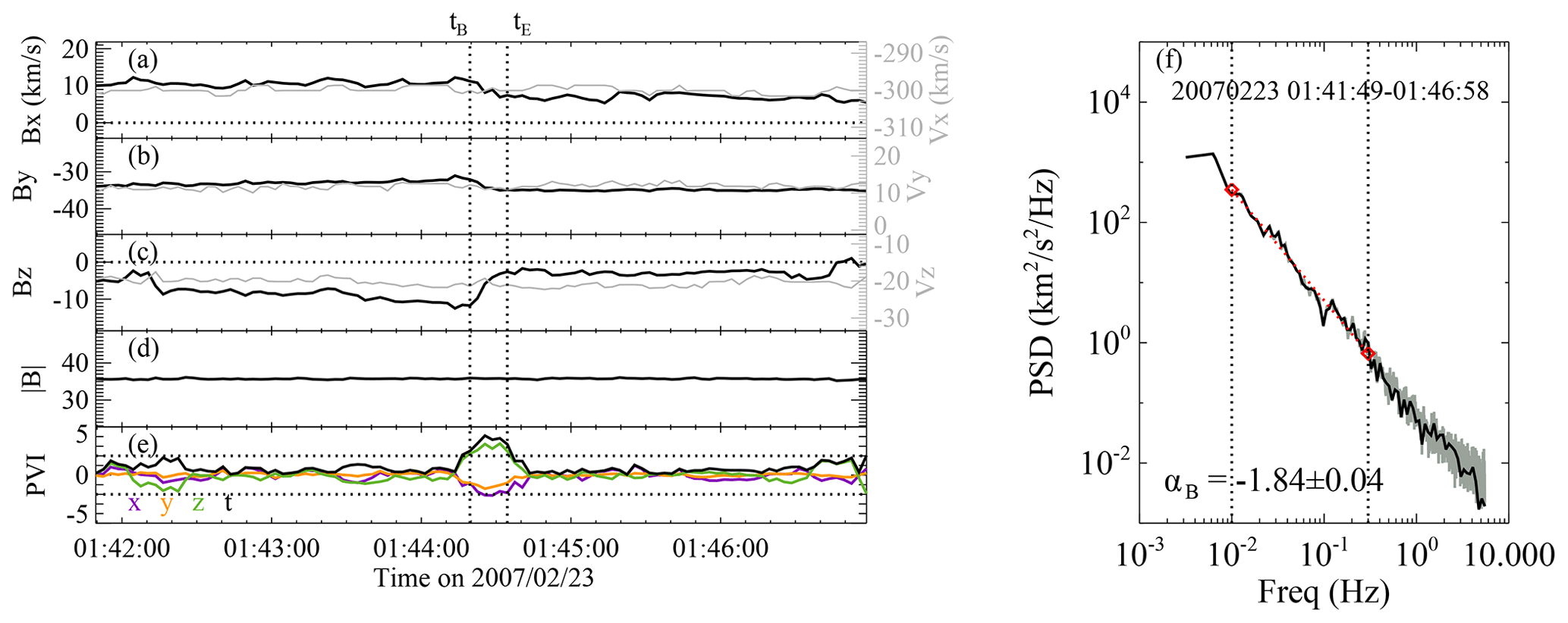
Figure 2 A typical case of an intermittent interval observed by the Wind spacecraft between 01:41:49 and 01:46:58 UT on 23 February 2007. (a–c) Time variations in the magnetic field vector (black) and the proton velocity vector (gray) in the GSE coordinates. The magnetic field is plotted in Alfvén units (i.e., $B/\sqrt{{\mathit{\mu }}_{\mathrm{0}}{m}_{\mathrm{p}}〈n_{\mathrm{p}}〉}$, where μ₀ is susceptibility, m_p is proton mass, and 〈n_p〉 is the average proton number density of this interval). (d) Magnetic field magnitude plotted in Alfvén units. (e) Normalized partial variance of increments (PVI) for the magnetic field vector at the timescale of τ=24 s, with PVI_x in purple, PVI_y in orange, PVI_z in green, and the matrix trace of the PVI in black. The two horizontal lines correspond to $\left|\mathrm{PVI}\right|=\mathrm{2}$, which was used to search for the intermittent structure. The two vertical dotted lines mark the beginning time (t_B) and the ending time (t_E) of the intermittent structure, respectively. (f) Spacecraft-frame trace power spectra of magnetic field fluctuations. The gray curve corresponds to the magnetic power spectrum obtained by performing FFT on the $\mathrm{1}/\mathrm{11}$ s resolution magnetic field data in Alfvén units, still using $\mathbf{B}/\sqrt{{\mathit{\mu }}_{\mathrm{0}}{m}_{\mathrm{p}}〈n_{\mathrm{p}}〉}$ with a simple rectangular window. The black curve superposed on the gray one corresponds to the uniformly distributed spectrum after interpolation. The magnetic spectral index and its uncertainty are obtained by applying a least-squares fit to the interpolated spectrum, resulting in the straight line (dotted red line) over the frequency range from 0.01 to 0.3 Hz (between the two vertical dotted lines).

Next, we determine the intermittency level for each interval. The trace of the normalized partial variance of increments is obtained from $I=\sqrt{({\mathrm{PVI}}_x{)}^{\mathrm{2}}+({\mathrm{PVI}}_y{)}^{\mathrm{2}}+({\mathrm{PVI}}_z{)}^{\mathrm{2}}}$. If the maximum I (I_max) during an intermittent structure (e.g., between the two vertical lines for the case shown in Fig. 2) is also the maximum I during the corresponding intermittent interval (e.g., the whole interval for the case shown in Fig. 2), this interval will be reserved, and I_max is recorded as the intermittency level of this case. Otherwise, the case is eliminated because the energy of the fluctuations during the interval is not dominated by the intermittent structure of interest. In the case shown in Fig. 2, we see that I_max=4.10 at 01:44:23 UT is also the maximum I within the plotted interval, so this case satisfies the condition well. In this way, 25 912 intermittent intervals are reserved for the following analysis.

We then perform fast Fourier transform (FFT) on the magnetic field fluctuations in Alfvén units and obtain the spectral index of the Fourier spectrum in the inertial range. In this procedure, we use high-resolution magnetic field data with $\mathrm{\Delta }{t}_{\mathrm{H}}=\mathrm{1}/\mathrm{11}$ s, so that the magnetic spectral index will be more reliable. The high-resolution magnetic field data are first transformed into Alfvén units (i.e., $B/\sqrt{{\mathit{\mu }}_{\mathrm{0}}{m}_{\mathrm{p}}〈n_{\mathrm{p}}〉}$, where 〈n_p〉 is the average proton number density of each interval). When converting the magnetic field into Alfvén units, we use one proton number density value that corresponds to the ensemble average of the proton number density 〈n_p〉 for each selected interval. By doing so, we avoid contamination of the magnetic spectral index value by noise in the density measurements, which would result from using a density value that changes every 3 s. For a given intermittent interval, the time series of each component of the high-resolution magnetic field data in Alfvén units is Fourier transformed using the FFT method with a simple rectangular window. This method could introduce extra discontinuity in the data that will add Fourier power to the magnetic power spectral density (PSD), as mentioned by Borovsky (2012) and Borovsky and Burkholder (2020). In Sect. 4.4, we linearly detrend the data prior to Fourier transformation, following Borovsky (2012), and make a comparison between the two methods. The trace of the magnetic spectral matrix gives the total power spectral density, and the magnetic spectrum is then smoothed using the three-point centered moving average following Wang et al. (2015). In Fig. 2f, we plot the magnetic PSD as a function of the spacecraft frequency (f) in log–log space, i.e., y=log ₁₀(PSD) versus x=log ₁₀(f), shown using the gray curve. We see that, using the high-resolution data, the magnetic spectrum can cover more than 3 orders of magnitude from $\mathrm{3.3}\times {\mathrm{10}}^{-\mathrm{3}}$ to 5.5 Hz.

It is known that the points of the gray spectrum shown in Fig. 2f are not uniformly distributed in the logarithmic space of f. As mentioned in Podesta (2016), the number of data points between two points (x and x+Δx) in this space increases exponentially with x. If a least-squares fit is performed, each point has equal weight. Therefore, the fit favors the points in the higher-frequency range, as this range contains more points (Podesta, 2016; Borovsky and Burkholder, 2020). In order to avoid this issue, we linearly interpolate the spectral density onto a uniformly spaced grid with $\mathrm{\Delta }x=(f_{\max }-f_{\min })/\mathrm{100}$ in the log–log space, following Podesta (2016). In Fig. 2f, the black curve superposed on the original gray spectrum demonstrates the interpolated spectrum.

We then perform a least-squares fit to the interpolated magnetic spectrum to obtain the magnetic spectral index α_B in the log–log space in the inertial range. The least-squares fit is performed in the frequency range between 0.01 and 0.3 Hz (between the two vertical dotted lines shown in Fig. 2f), and the magnetic spectrum can be fitted well by a straight line with a slope of α_B in this range. The slope (α_B) and its corresponding error (${\mathrm{\Delta }}_{{\mathit{\alpha }}_B}$) are obtained (and both marked in Fig. 2f) as ${\mathit{\alpha }}_B=-\mathrm{1.84}\pm \mathrm{0.04}$. We perform the same analysis on all of the selected intervals. The cases with a relative fitting error ${\mathrm{\Delta }}_{{\mathit{\alpha }}_B}/{\mathit{\alpha }}_B>\mathrm{5}\mathit{\%}$ are eliminated, as their magnetic spectra do not have a good power-law shape and cannot be fitted well by a straight line in the log–log space at the frequency range of interest. Finally, 24 886 intermittent intervals are reserved for the following statistical analysis in order to explore the relation between the magnetic spectral index α_B and the intermittency level I_max.

3 Results: variations in the magnetic spectral index versus the intermittency level

For the 24 886 selected cases, we first present the joint distribution of their width in units of data points and intermittency level I_max in Fig. 3a. Here, the width in units of data points for an intermittent structure is obtained from t_E−t_B, during which the condition $\left|{\mathrm{PVI}}_i\right|>\mathrm{2}$ satisfies (i=x, y, or z), divided by the time resolution Δt=3 s. We see that most of the cases have the following values: $\mathrm{5}\le \mathrm{width}<\mathrm{7}$ and $\mathrm{3}\le I_{\max }<\mathrm{6}$. As the width increases, the distribution of I_max extends to a wider range. This phenomenon makes the pattern of the joint distribution look like a triangle, which is consistent with Miao et al. (2011). In their Fig. 8, the aforementioned authors show the triangle-like shape of the 2D distribution in the Δθ−τ plane, where Δθ and τ are the deflection angle across the current sheet and the width of the current sheet, respectively. Figure 3b shows the probability distribution of the width for the intermittent structures of interest. The width extends from 3 (9 s) to 20 data points (60 s), and the most probable value is 5 data points (15 s). As the width increases, the probability distribution function first increases immediately and then decreases gradually. Figure 3c shows the probability distribution of the intermittency level I_max. The value of I_max extends from about 2 to 15, and the most probable value is 4.5. The profile of the distribution is similar to that of the width.

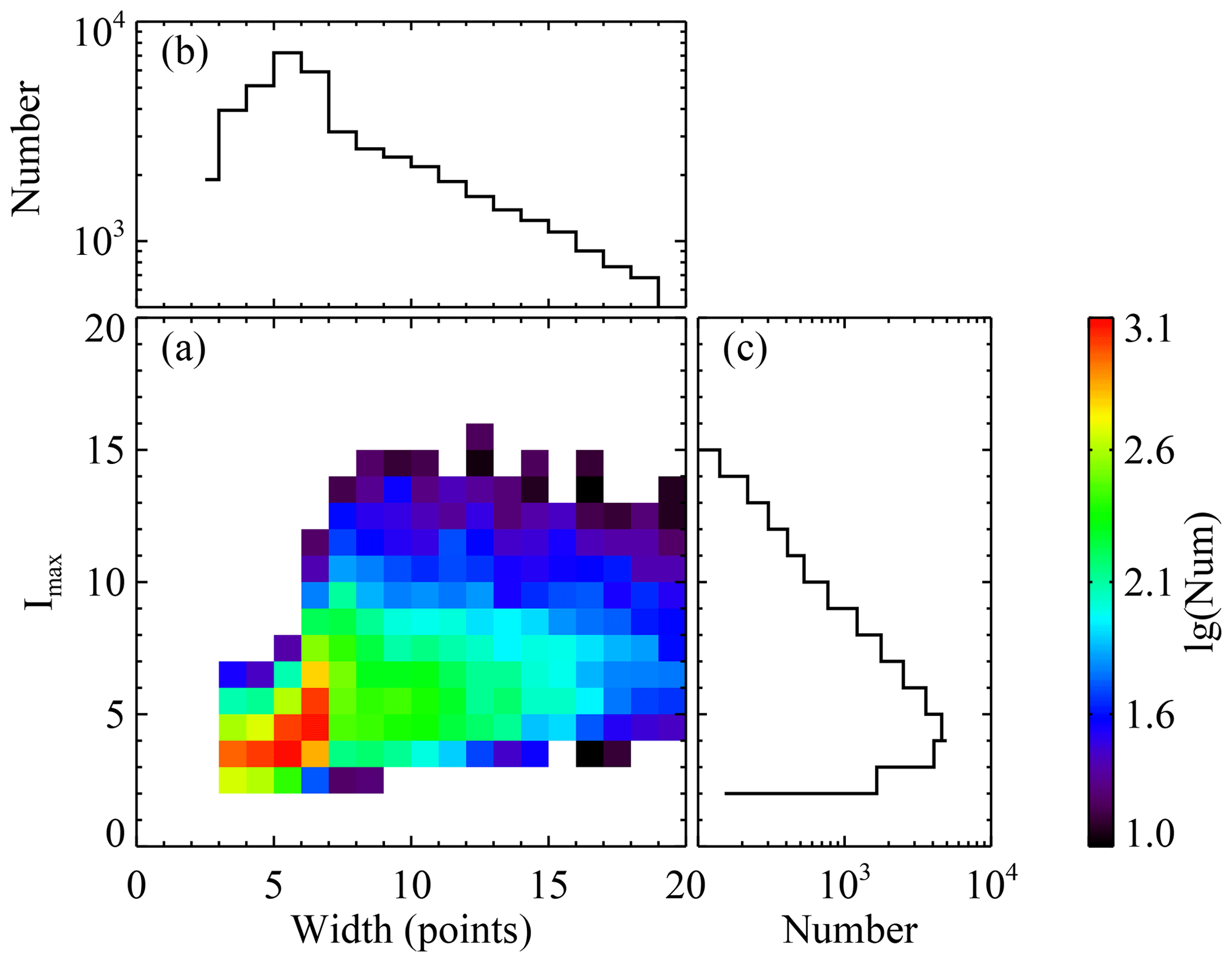
Figure 3 (a) Joint distribution of width in units of data points and intermittency level (I_max) for the 24 886 selected intermittent structures. The width in units of data points for an intermittent structure is obtained from t_E−t_B, during which the condition $\left|{\mathrm{PVI}}_i\right|>\mathrm{2}$ satisfies (i=x, y, or z), divided by the time resolution Δt=3 s. The pixels containing no more than 10 cases are ignored. Panels (b) and (c) show the probability distribution of the width and of the intermittency level (I_max), respectively.

Another typical intermittent interval observed on 12 September 2010 is shown in Fig. 4, although with a higher intermittency level I_max=13.09. Figure 4 is plotted in the same format as Fig. 2. The intermittent structure is marked by the two vertical dotted lines. Between the two vertical lines, the time instants all satisfy at least one of the abovementioned conditions: $\left|{\mathrm{PVI}}_x\right|>\mathrm{2}$, $\left|{\mathrm{PVI}}_y\right|>\mathrm{2}$, or $\left|{\mathrm{PVI}}_z\right|>\mathrm{2}$. Between t_B and t_E, a large jump happens in both the x and z components of the magnetic field. The fluctuations in the proton velocity (in gray) are well correlated with the fluctuations in the magnetic field (correlation coefficient of cc=0.97). However, the fluctuation amplitude of the proton velocity is much smaller than the magnetic field (normalized residual energy of ${\mathit{\sigma }}_{\mathrm{r}}=-\mathrm{0.50}$). This indicates that this may be a magnetic–velocity alignment structure (Wang et al., 2020; Wu et al., 2021). Magnetic–velocity alignment structures, the generation mechanism of which remains unclear, are a kind of magnetically dominated structure but with a high correlation between the magnetic field fluctuations and velocity fluctuations. For these kinds of structures, the magnetic field fluctuations are nearly aligned with the velocity fluctuations.

For the case shown in Fig. 4, the intermittency level I_max is recorded as 13.09, which corresponds to the value of I at 06:28:48 UT. Figure 4f shows the power spectrum of magnetic field fluctuation obtained by performing FFT on the high-resolution magnetic field data. The original spectrum before interpolation is still plotted in gray, and the uniformly distributed spectrum after interpolation in black is superposed on the gray one. A least-squares fit is performed on the interpolated spectrum at the frequency range between 0.01 and 0.3 Hz. The spectral index is obtained as ${\mathit{\alpha }}_B=-\mathrm{2.01}\pm \mathrm{0.04}$. The small fitting error indicates that the magnetic spectrum has a good power-law shape. The magnetic spectral index obtained here is very close to −2. Thus, it is very consistent with previous theory and observations, which proposed that the discontinuities can produce an f⁻² energy spectrum in the inertial range (Sari and Ness, 1969; Roberts and Goldstein, 1987; Champeney, 1973; Dallas and Alexakis, 2013).

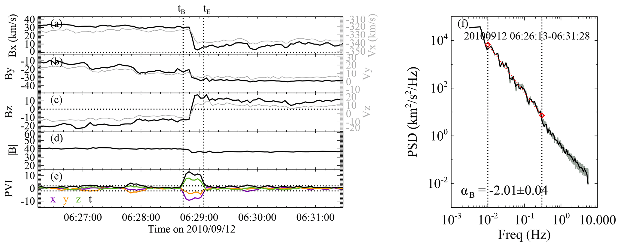
Figure 4 A typical case of an intermittent interval observed by the Wind spacecraft between 06:26:13 and 06:31:28 UT on 12 September 2010, displayed in the same format as Fig. 2.

However, as seen from the case with ${\mathit{\alpha }}_B=-\mathrm{1.84}\pm \mathrm{0.04}$, shown in Fig. 2, the discontinuities are not always related to a −2 magnetic spectral index in the solar wind observations. The case shown in Fig. 2 also has a typical discontinuity embedded in the background turbulence, but its intermittency level (I_max=4.10) is relatively smaller than that shown in Fig. 4 (I_max=13.09). Correspondingly, the magnetic spectrum of the case shown in Fig. 2 is shallower. Therefore, it is clear that the intermittency level can significantly affect the spectral index of the magnetic field fluctuations in the inertial range. It is necessary to know the analytical relation between the intermittency level and the magnetic spectral index.

In order to give the continuous variation in the magnetic spectral index as a function of the intermittency level, we also select some “quiet” intervals with $\left|{\mathrm{PVI}}_i\right|<\mathrm{2}$. In this procedure, we first cut the data in the 46 slow-wind streams into short intervals with a duration of 5 min. We then check the maximums of $\left|{\mathrm{PVI}}_x\right|$, $\left|{\mathrm{PVI}}_y\right|$, and $\left|{\mathrm{PVI}}_z\right|$ in each interval, respectively. If their maximums are all smaller than 2, the interval is reserved as a quiet interval. During a given interval, the maximum of the trace $I=\sqrt{({\mathrm{PVI}}_x{)}^{\mathrm{2}}+({\mathrm{PVI}}_y{)}^{\mathrm{2}}+({\mathrm{PVI}}_z{)}^{\mathrm{2}}}$ is recorded as the “intermittency level” (I_max), although it may not be intermittent at all. Their magnetic spectral indices are also obtained using the method mentioned above. Subsequently, we find 17 386 quiet cases for the following study.

Figure 5 shows (using the same format as Fig. 2) a typical quiet interval with very low intermittency level of I_max=1.44. The magnetic power spectrum is much shallower than that of the intermittent intervals with relatively higher intermittency levels shown in Figs. 2 and 4. The magnetic spectral index comes out to be $-\mathrm{1.65}\pm \mathrm{0.04}$. It seems to be close to the Kolmogorov scaling of $f^{-\mathrm{5}/\mathrm{3}}$. We check the Alfvénicity of this case and find that it is not an Alfvénic interval with a low normalized cross helicity of σ_c=0.34 and a low Alfvén ratio of γ_A=0.47. It is worth noting that an intermittency correction could be considered if the magnetic spectrum scales as $f^{-\mathrm{5}/\mathrm{3}}$ for an Alfvénic interval.

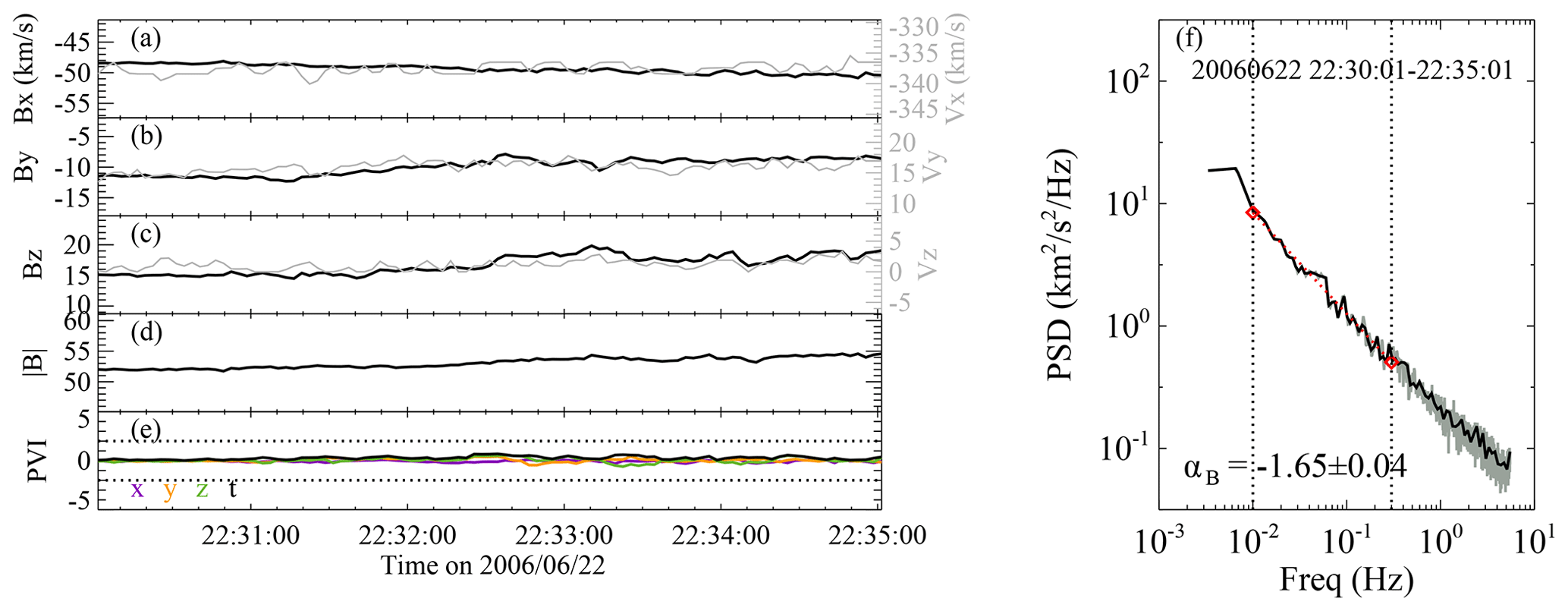
Figure 5 A typical case of a quiet interval observed by the Wind spacecraft between 22:30:01 and 22:35:01 UT on 22 June 2006, shown in the same format as Fig. 2. The fluctuation amplitude of the proton velocity (gray curves in panels a, b, and c) is very close to the instrument noise level (2 km s⁻¹) in the 3DP velocity observations (Wicks et al., 2013a). Thus, the variations in the proton velocity look noisy here.

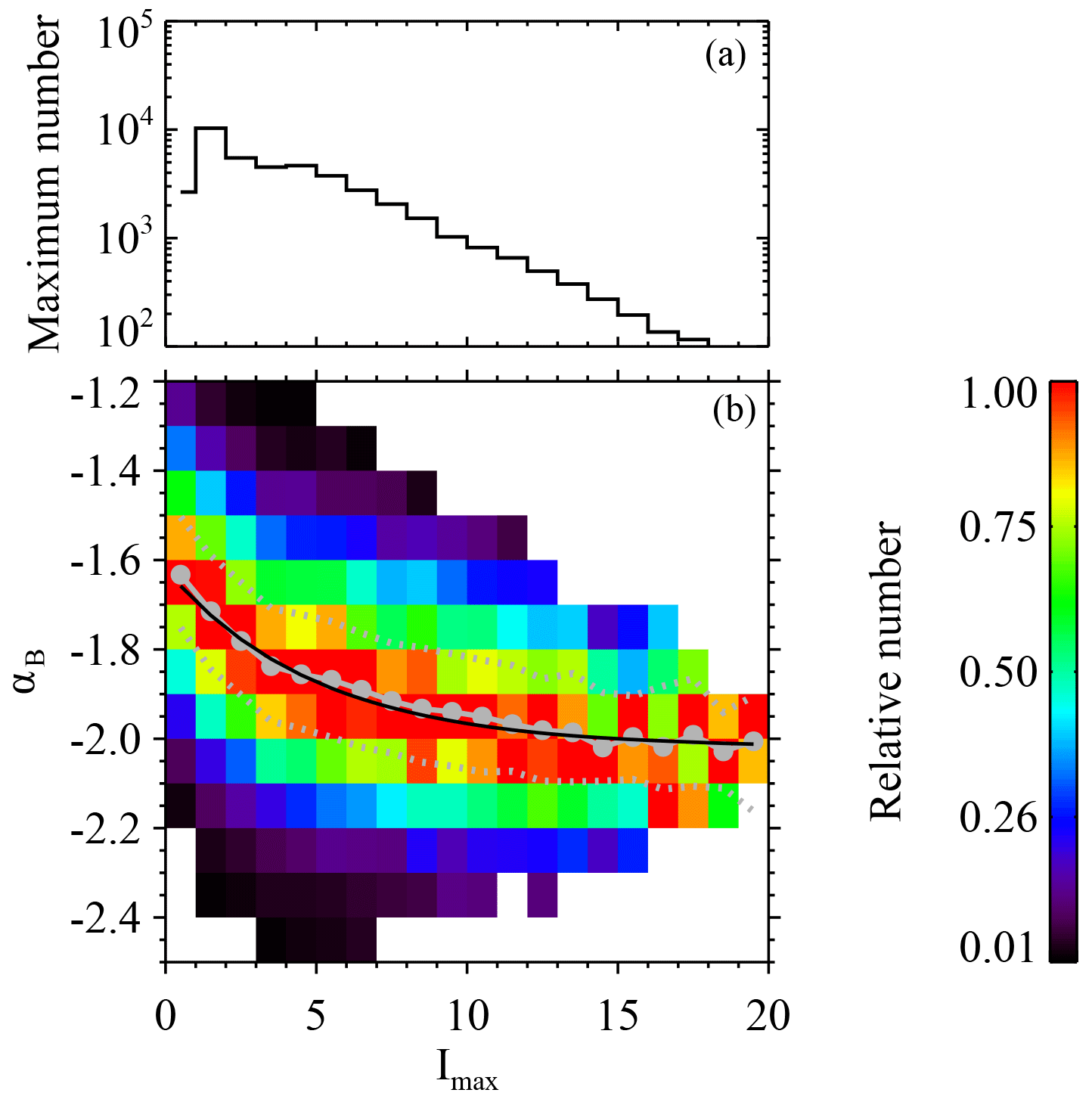
Figure 6 Joint distribution of the intermittency level I_max and magnetic spectral index α_B for the 42 272 selected intervals. The bin width of I_max is 1, and the bin width of α_B is 0.1. For a given pixel, the color denotes the relative number, which is the number of cases normalized by the maximum number in the corresponding column (I_max bin). The maximum number in each bin is shown in panel (a). The pixels containing no more than 10 cases are ignored. The solid gray circles represent the average α_B in each I_max bin. The dotted gray lines represent the upper/lower quartiles. The black curve, corresponding to the exponential function ${\mathit{\alpha }}_B=\mathrm{0.4}\exp (-I_{\max }/\mathrm{5})-\mathrm{2.02}$, represents the fitting result to the solid gray circles.

Figure 6b shows the joint distribution of I_max and α_B for the 42 272 selected intervals. The x axis, corresponding to the intermittency level I_max in the range [0,20], is divided into 20 bins. The y axis, corresponding to the magnetic spectral index α_B in the range $[-\mathrm{2.5},-\mathrm{1.2}]$, is divided into 13 bins. For a given pixel, the color denotes the number of cases normalized by the maximum number of pixels in the corresponding I_max bin. Thus, in each column, the pixel with the largest number of cases is colored in red, corresponding to 1. The maximum number in each column versus I_max is also shown in Fig. 6a. In order to guarantee that there are enough cases used for the statistics, the pixels containing no more than 10 cases are ignored. Therefore, the pixels in black contain the smallest number of cases, but the number of cases is still larger than 10. If we focus on the pixels in red, we notice that the magnetic spectral index α_B has a very clear decreasing trend from $\sim -\mathrm{1.6}$ to $\sim -\mathrm{2}$ as the intermittency level I_max increases. The solid gray circles show the average α_B in each I_max bin as a function of I_max, and the dotted gray lines represent the upper/lower quartiles. It is found that the magnetic power spectrum gets steeper quickly from $f^{-{\mathrm{1.63}}_{-\mathrm{0.12}}^{+\mathrm{0.09}}}$ to $f^{-{\mathrm{1.84}}_{-\mathrm{0.11}}^{+\mathrm{0.14}}}$ as I_max increases from 0.5 to 3.5. When I_max increases from 4.5 to 15.5, the magnetic power spectrum gets steeper slowly from $f^{-{\mathrm{1.86}}_{-\mathrm{0.11}}^{+\mathrm{0.14}}}$ to $f^{-{\mathrm{1.99}}_{-\mathrm{0.11}}^{+\mathrm{0.09}}}$. As I_max>16, the magnetic spectral index remains close to −2.

The observed variation in the magnetic spectral index α_B versus the intermittency level I_max can be well fitted by an exponential function. In Fig. 6, the black curve corresponding to ${\mathit{\alpha }}_B=\mathrm{0.4}\exp (-I_{\max }/\mathrm{5})-\mathrm{2.02}$ shows the fitting result. This empirical relation supplies the continuous variation in the spectral index α_B of the magnetic field in the inertial range as a function of the intermittency level I_max. The empirical relation tells us that the magnetic spectral index in the inertial range will be close to −1.6 when I_max is small (and the fluctuations in the magnetic field could be considered to be randomly distributed). As the fluctuations become intermittent, the magnetic spectrum gradually becomes steeper until $\sim f^{-\mathrm{2}}$.

4 Discussion

Our result confirms the idea that intermittent structures have a significant influence on the magnetic spectral index and often make the spectra become steeper (Siscoe et al., 1968; Burlaga, 1968; Salem et al., 2007, 2009). It is generally acknowledged that the time series of discontinuities produce an f⁻² energy spectrum in the inertial range. More recently, researchers have found that discontinuities can also produce shallower magnetic spectra (Li et al., 2011; Borovsky, 2010). In previous studies, discontinuities in the solar wind have been identified mainly as rotational discontinuities (e.g., Neugebauer et al., 1984; Tsurutani and Ho, 1999; Wang et al., 2013; Liu et al., 2021). However, in some other studies, discontinuities have been identified mainly as tangential discontinuities, depending on the different techniques used for data analysis (e.g., Horbury et al., 2001; Knetter et al., 2004; Riazantseva et al., 2005). Here, from the continuous relation, we find that f⁻² scaling could be produced if the intermittency level of the structure embedded in the turbulence was high enough, i.e., I_max>15 for the cases studied in this work. We have examined whether the intermittency level I_max could be biased by the anisotropy of fluctuations. It was found that the intermittency level I_max appears not to be dependent on the direction of the predominant fluctuations (figure not shown here, as it is similar to Fig. 9 shown below).

Our result is also consistent with the radial evolution trend in intermittency and the magnetic spectral index in the solar wind. The evolution of intermittency with distance from the Sun can be explained on the basis of the interplay between coherent (intermittent) structures and Alfvénic fluctuations. Intermittent events advected by the wind are increasingly exposed as Alfvénic fluctuations are depleted with the heliocentric distance (see, e.g., Bruno et al., 2003). Using the observations from the Parker Solar Probe, researchers have also found that there is a clear transition for the magnetic spectral index in the inertial range as the radial distance from the Sun increases (Chen et al., 2020). When r≈0.17 AU, the magnetic spectral index is close to $-\mathrm{3}/\mathrm{2}$. When r≈0.6 AU, the magnetic spectrum becomes steeper as $\mathit{\alpha }\approx -\mathrm{5}/\mathrm{3}$. These observational results indicate that the solar wind turbulence becomes more intermittent as r increases and that the magnetic spectrum gets steeper. The variation trend in the magnetic spectral index versus the intermittency is confirmed by our observations. Recently, several papers have been published on scaling properties and intermittency levels with respect to the Parker Solar Probe (e.g., Alberti et al., 2020; Cuesta et al., 2022; Sioulas et al., 2022).

We also notice that the magnetic spectral index of the intervals for the cases with a very low intermittency level $\mathrm{0}<I_{\max }<\mathrm{1}$ is between −1.62 and −1.69, which is close to the Kolmogorov scaling. This is different from Li et al. (2011), who found that current-sheet-free periods show $f^{-\mathrm{3}/\mathrm{2}}$ Iroshnikov–Kraichnan scaling. From Fig. 6, we see that some of the low-intermittency-level cases can also produce $f^{-\mathrm{3}/\mathrm{2}}$ scaling, but the cases with $-\mathrm{1.6}<{\mathit{\alpha }}_B<-\mathrm{1.4}$ only account for 20 % of all of the cases with I_max<1. The differences between this work and Li et al. (2011) include the following: (1) the aforementioned authors focus on the ∼ 1 d Ulysses data at about 5 AU, whereas we use the 5 min Wind data at about 1 AU; (2) the frequency range for the fit is [${\mathrm{10}}^{-\mathrm{3}},{\mathrm{10}}^{-\mathrm{1}}$] Hz in Li et al. (2011), whereas it is [0.01,0.3] Hz here.

f⁻² scaling has been reported for parallel-sampling magnetic fluctuations in many previous studies associated with magnetic spectral anisotropy (Horbury et al., 2008; Podesta, 2009; Luo and Wu, 2010; Chen et al., 2011; Forman et al., 2011; Wicks et al., 2011). Wang et al. (2014) found that the magnetic spectrum in the parallel direction becomes shallower from f⁻² to $f^{-\mathrm{5}/\mathrm{3}}$ after removing the intermittency. However, the question regarding how intermittency affects the anisotropy of the magnetic spectral index remains unclear. In the future, we might try to check the intermittency level of the parallel-sampling data to see if the steep spectrum in the parallel direction is related to a high intermittency level or not.

Intermittency in many theoretical models has also been found to steepen the inertial-range power spectrum of turbulence. For example, a multifractal model developed by She and Leveque (1994) (SL model) provided intermittency correction to the Kolmogorov law (Kolmogorov, 1941) and predicted an energy spectrum of $E\left(k\right)\approx k^{-\mathrm{5}/\mathrm{3}-\mathrm{0.03}}$ for fluids. Carbone (1993) presented a magnetohydrodynamic (MHD) cascade model and provided an intermittency modification to the Kraichnan theory. Politano and Pouquet (1995) extended the SL model to the MHD case, and the energy spectrum was obtained as $E\left(k\right)\approx k^{-\mathrm{3}/\mathrm{2}-\mathrm{0.04}}$. For the velocity spectrum, Boldyrev et al. (2002) predicted $E\left(k\right)\approx k^{-\mathrm{1.74}}$ from an analytical study of driven supersonic MHD turbulence. Recently, Chandran et al. (2015) found that the power spectrum of the intermittent turbulence flattens when considering scale-dependent dynamic alignment. However, there seems to be no conclusion regarding which model is the most appropriate one to describe the solar wind turbulence. According to the observational result shown in this work with respect to the slow-wind streams, we obtain an empirical relation between the magnetic spectral index α_B and the intermittency level I_max. This relation will supply an observational basis for theoretical studies of the intermittent turbulence and will help improve the turbulence theory related to the slow solar wind.

4.1 Influence of magnetic compressibility

Besides intermittency, the magnetic spectral index has been reported to also depend on the level of magnetic compressibility. Magnetic compressibility has been defined as the ratio between the variance in the magnetic field magnitude fluctuations and the variance matrix trace of the fluctuations, i.e., $c_b={\mathit{\sigma }}_{\left|B\right|}^{\mathrm{2}}/{\sum }_{i=x,y,z}{\mathit{\sigma }}_{B_i}^{\mathrm{2}}$ (Bavassano et al., 1982; Telloni et al., 2019; Wang et al., 2020). Here, in order to take the influence of the magnetic compressibility on the shape of the magnetic spectrum into account, we also calculate the magnetic compressibility of all of the 24 886 intermittent intervals and the 17 386 quiet intervals in the 46 slow-wind streams.

Figure 7b shows (in the same format as Fig. 6) the joint distribution of the magnetic compressibility c_b and α_B for the 24 886 selected intermittent intervals. The x axis, corresponding to the magnetic compressibility c_b in the range [0,0.5], is divided into 20 bins. The y axis, corresponding to the magnetic spectral index α_B in the range $[-\mathrm{2.5},-\mathrm{1.2}]$, is still divided into 13 bins. For a given pixel, the color also denotes the number of cases normalized by the maximum number of pixels in the corresponding c_b bin. The maximum number in each column versus c_b is also shown in Fig. 7a. The pixels containing no more than 10 cases are ignored. When we focus on the pixels in red, we notice that the magnetic spectral index α_B remains almost constant as c_b increases. The solid gray circles show the average α_B in each c_b bin, and the two dotted gray lines represent the respective upper and lower quartiles. For the selected intermittent intervals, it is found that the average slope of the magnetic spectrum in the inertial range varies between $[-\mathrm{1.90},-\mathrm{1.80}]$ as the magnetic compressibility c_b increases from 0 to 0.5 and that there is no systematic trend. This result could indicate that, for the intermittent cases, the magnetic compressibility does not have significant influence on the magnetic spectral index in the slow-wind streams of interest.

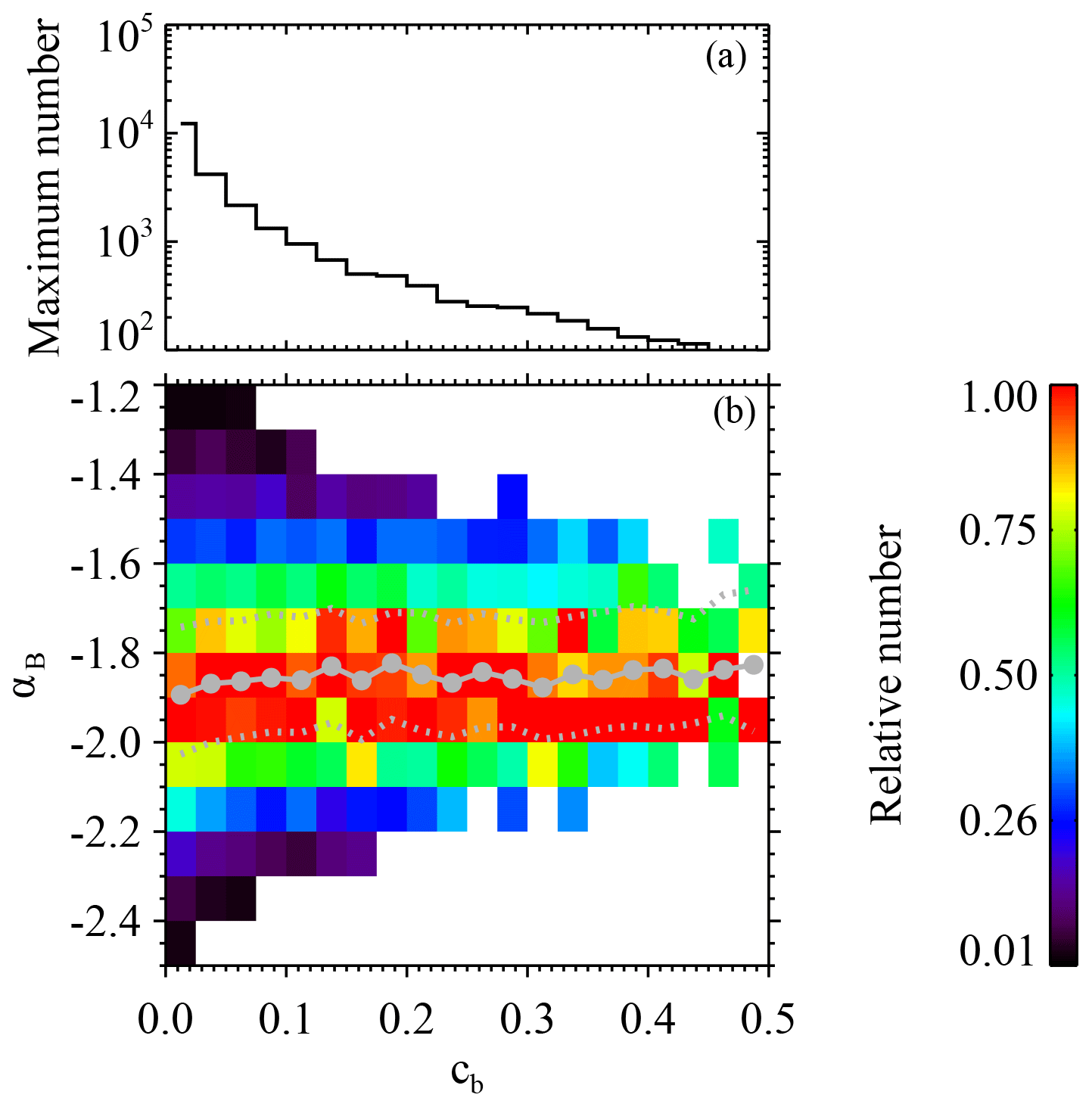
Figure 7 Joint distribution of the magnetic compressibility c_b and magnetic spectral index α_B for the 24 886 selected intermittent intervals, shown in the same format as Fig. 6.

The same analysis is performed on the 17 386 selected quiet intervals. The result is shown in Fig. 8. Figure 8 is plotted in the same format as Fig. 7. When we focus on the most probable value of α_B in each c_b bin, i.e., the pixels in red, we also find that no clear trend appears. The solid gray circles and the two dotted gray lines represent the average α_B in each c_b bin and the upper/lower quartiles, respectively. When c_b increases from 0 to 0.5, the magnetic spectral index changes slightly from $-\mathrm{1.76}\pm \mathrm{0.14}$ to $-\mathrm{1.70}\pm \mathrm{0.10}$. This result indicates that, for the quiet cases in the slow-wind streams of interest, the magnetic compressibility also does not significantly affect the magnetic spectral index.

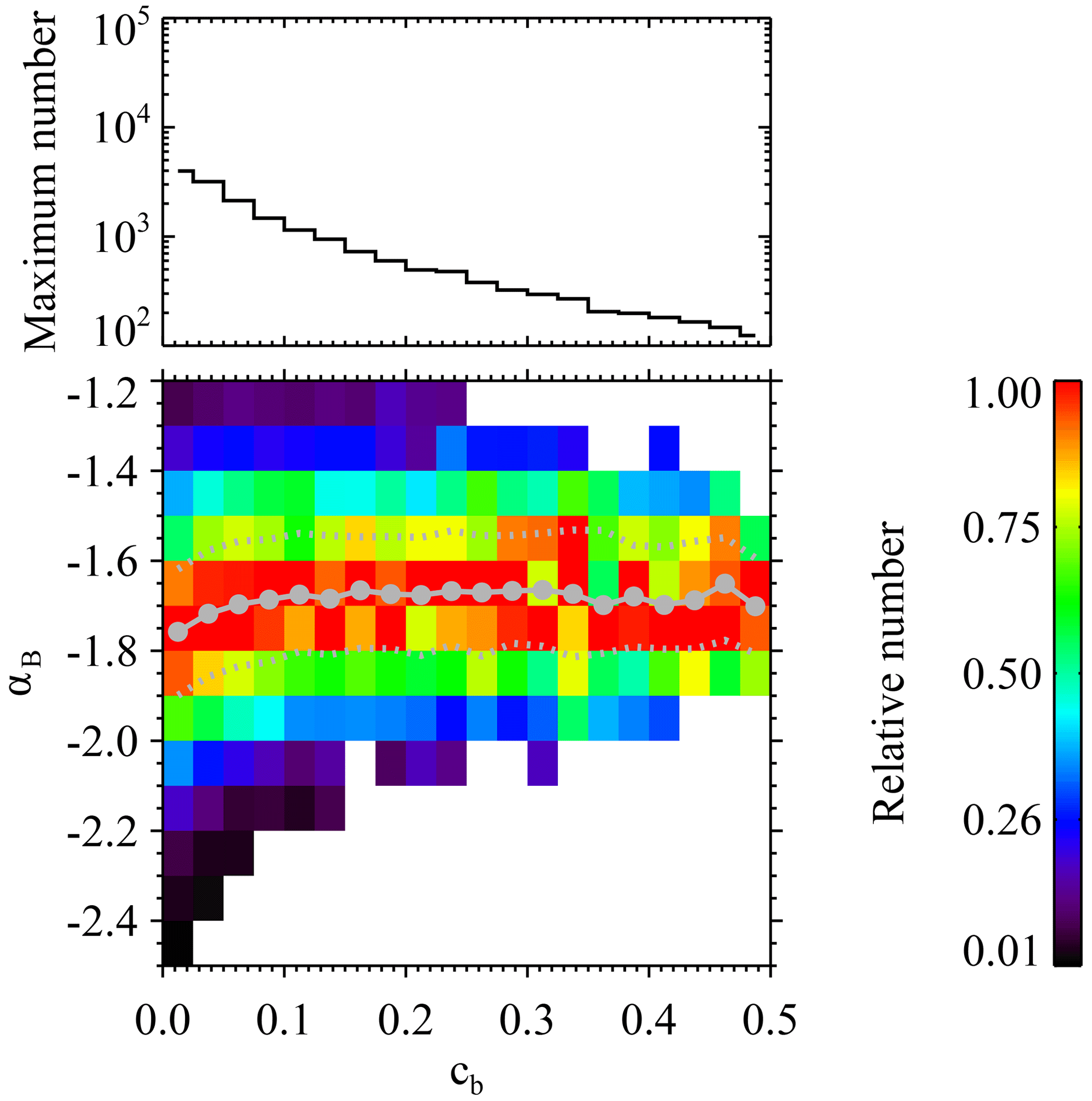
Figure 8 Joint distribution of the magnetic compressibility c_b and magnetic spectral index α_B for the 17 386 selected quiet intervals, shown in the same format as Fig. 6.

4.2 Influence of anisotropy of magnetic field fluctuations

As different spectral indices are observed in different directions with respect to the mean field, as mentioned in Sect. 1, it is necessary to reveal how the presented results shown in Fig. 6 could be biased by the anisotropy of magnetic field fluctuations. Thus, we perform a check to see if the spectral slope is dependent on the predominance of fluctuations in a specific direction. Here, the direction of the predominant fluctuations is indicated by the maximum variance (L) direction, which is obtained via minimum variance analysis (Sonnerup and Cahill, 1967). In Fig. 9, we show the variations in the magnetic spectral index as a function of the angle between the L and i direction (θ_Li) (where i denotes the x axis, y axis, and z axis of GSE coordinates) as well as the variations in the spectral index versus the angle between L and the mean magnetic field direction of each interval (θ_LB).

Figure 9a2 shows the variation in the magnetic spectral index α_B as a function of θ_LX. The angle ${\mathit{\theta }}_{LX}\sim \mathrm{0}{}^{\circ }$ means that the predominant fluctuations in the intermittent structure are mainly focused in the x direction, whereas ${\mathit{\theta }}_{LX}\sim \mathrm{90}{}^{\circ }$ means that they are mainly focused in the plane perpendicular to the x direction. Only 79 % of the selected intervals with ${\mathit{\lambda }}_{\mathrm{1}}/{\mathit{\lambda }}_{\mathrm{2}}>\mathrm{3}$ remain for the analysis, where λ₁ and λ₂ are the eigenvalues corresponding to the maximum variance direction and the intermediate variance direction, respectively. This condition guarantees that the maximum variation direction is determined precisely, and the fluctuations in the L direction are distinctly dominant in each interval. Figure 9a1 and a2 are plotted in a similar format to Fig. 6. For a given pixel in Fig. 9a2, the color denotes the number of cases normalized by the maximum number in the corresponding θ_LX bin, and the maximum number in each bin is shown in Fig. 9a1. The solid gray circles represent the average α_B in each θ_LX bin. The dotted gray lines represent the upper/lower quartiles. The solid gray circles show that there is a slight decreasing trend for the average spectral index α_B (from −1.76 to −1.86) as θ_LX increase from 0^∘ to 90^∘. However, if we consider the quartiles (i.e., from $-{\mathrm{1.76}}_{-\mathrm{0.10}}^{+\mathrm{0.14}}$ to $-{\mathrm{1.86}}_{-\mathrm{0.14}}^{+\mathrm{0.13}}$), the slight trend is nearly negligible. Therefore, the magnetic spectral indices of the intervals with the predominant fluctuations parallel or perpendicular to the x direction are not significantly different.

Figure 9b, c, and d show the variation in the magnetic spectral index as a function of θ_LY, θ_LZ, and θ_LB, respectively. A slight increasing trend (from $-{\mathrm{1.89}}_{-\mathrm{0.17}}^{+\mathrm{0.17}}$ to $-{\mathrm{1.84}}_{-\mathrm{0.13}}^{+\mathrm{0.14}}$) appears in Fig. 9b2, but the trend is also not significant, considering the errors. In Fig. 9c2, the average α_B (solid gray circles) remains almost constant at −1.85. In Fig. 9d2, the average α_B (solid gray circles) varies with θ_LB, and no clear trend exists.

According to the results presented in Fig. 9, we suggest that the influence of the anisotropy of the predominant fluctuations on the magnetic spectral index is not as significant as the influence of the intermittency level I_max on the index (when I_max increases from 0 to 20, α_B decreases from −1.63 to −2.01).

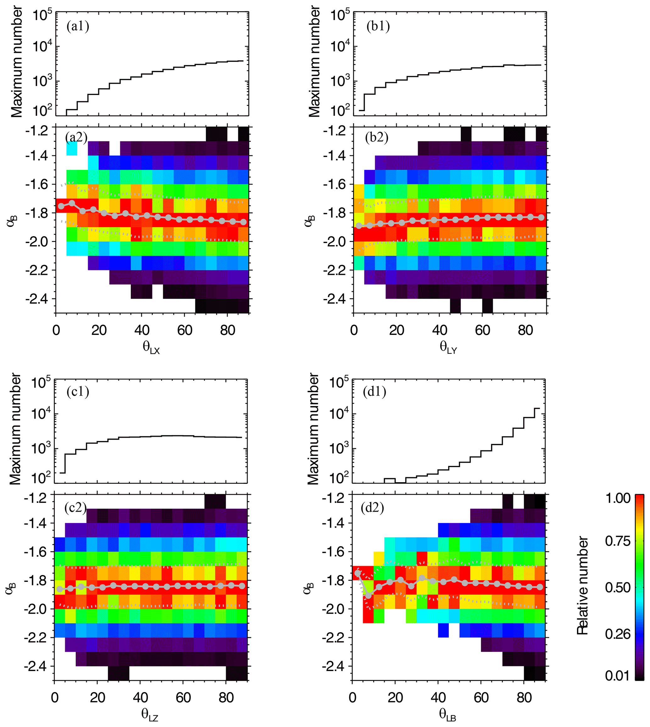
Figure 9 (a2) Joint distribution of θ_LX and the magnetic spectral index α_B for the 33 261 intervals with ${\mathit{\lambda }}_{\mathrm{1}}/{\mathit{\lambda }}_{\mathrm{2}}>\mathrm{3}$. For a given pixel, the color denotes the relative number, which is the number of cases normalized by the maximum number in the corresponding θ_LX bin. The maximum number in each bin is shown in panel (a1). The pixels containing no more than 10 cases are ignored. The solid gray circles represent the average α_B in each θ_LX bin. The dotted gray lines represent the upper/lower quartiles. Panels (b1) and (b2) are plotted in the same format as panels (a1) and (a2) but for θ_LY. Panels (c1) and (c2) correspond to θ_LZ. Panels (d1) and (d2) correspond to θ_LB.

4.3 Coincidence between the intermittency level and multifractal width

As shown in the literature (e.g., Frisch, 1995; Veltri and Mangeney, 1999; Salem et al., 2009), intermittency is strictly related to multifractality, which is measured by looking at the high-order scaling properties. Therefore, it is necessary to check if the I_max used here is consistent with multifractal indicators of intermittency, such as the multifractal width introduced in a series of work by Macek et al. (2005, 2009, 2012).

The multifractal properties can be described by the multifractal singularity spectrum of the observed time sequence. The width of the spectrum represents the extent of multifractality. Here, we estimate the multifractal singularity spectrum of the magnetic field fluctuations using the classical approach following previous studies (Paladin and Vulpiani, 1987; Macek et al., 2005; Macek and Wawrzaszek, 2009; Macek et al., 2012; Marsch et al., 1996; Burlaga, 1991a; Burlaga et al., 2006; Sorriso-Valvo et al., 2017). For each selected interval, we perform a multifractal analysis on the time sequence of the magnetic field fluctuations in the maximum variance direction (B_L(t)) with a high time resolution of $\mathrm{\Delta }{t}_{\mathrm{H}}=\mathrm{1}/\mathrm{11}$ s. The increment of B_L(t) is $\mathrm{\Delta }{B}_L\left(t\right)=\left|B_L\right(t+\mathrm{d}t)-B_L(t\left)\right|$, where dt=10 s belongs to the inertial range. The time series ΔB_L(i) ($i=\mathrm{1},\mathrm{2},\mathrm{\dots },N$, where $N=T/\mathrm{\Delta }{t}_{\mathrm{H}}$ and T is the duration of each interval) is divided into subsets of variable scale Δ s, with $j=\mathrm{1},\mathrm{2},\mathrm{\dots },M$ ($M=T/\mathrm{\Delta }s$). A logarithmically spaced range of eight timescales $\mathrm{10}/\mathrm{11}$ s $<\mathrm{\Delta }s<\mathrm{150}$ s is used. For each subset, the generalized probability measure is defined as follows:

$$\begin{array}{}\text{(2)}& {\mathit{\mu }}_j\left(\mathrm{\Delta }s\right)={\displaystyle \frac{{\sum }_{i=(j-\mathrm{1})\mathrm{\Delta }s+\mathrm{1}}^{j\mathrm{\Delta }s}\left|\mathrm{\Delta }{B}_L\right(i\left)\right|}{{\sum }_{i=\mathrm{1},N}\left|\mathrm{\Delta }{B}_L\right(i\left)\right|}}.\end{array}$$

For a given q, we calculate the q-order total probability measure, and it scales as follows:

$$\begin{array}{}\text{(3)}& {\mathit{\chi }}_q\left(\mathrm{\Delta }s\right)=\sum _{j=\mathrm{1}}^M\mathrm{\Delta }s\left|{\mathit{\mu }}_j\right(\mathrm{\Delta }s){|}^q\propto (\mathrm{\Delta }s{)}^{{\mathit{\tau }}_q},\end{array}$$

where $q\in [-\mathrm{5},\mathrm{5}]$ with a step $\mathrm{d}q=\mathrm{1}/\mathrm{3}$ (similar to Sorriso-Valvo et al., 2017). The scaling exponent τ_q is obtained by performing a linear fit of χ_q(Δ s) versus Δ s in the inertial range [8 s, 100 s] on a log–log plot. We then obtain the singularity spectrum from $f\left(\mathit{\alpha }\right)=q{\mathit{\alpha }}_q-{\mathit{\tau }}_q$ and ${\mathit{\alpha }}_q=\mathrm{d}{\mathit{\tau }}_q/\mathrm{d}q$ (Halsey et al., 1986). Figure 10a presents the variations in f(α) versus α, with red denoting the intermittent interval shown in Fig. 4 (I_max=13.09), black denoting the intermittent interval shown in Fig. 2 (I_max=4.10), and blue denoting the quiet interval shown in Fig. 5 (I_max=1.44). The dots and solid lines represent the observational results and cubic polynomial fit to them, respectively.

A quantitative description of the degree of multifractality is the width of the singularity spectrum $\mathrm{\Delta }\mathit{\alpha }={\mathit{\alpha }}_{\max }-{\mathit{\alpha }}_{\min }$. We estimate α_min and α_max by fitting the observed values of (α,f(α)) with the cubic polynomial and extrapolating to f(α)=0, as shown in Fig. 10a. We find that the multifractal widths of the two intermittent intervals (Δα=1.19 in red and Δα=1.16 in black) are both much larger than that of the quiet interval (Δα=0.81 in blue). Moreover, the intermittent interval with a higher level of intermittency (I_max=13.09) shown in red also corresponds to a wider singularity spectrum (Δα=1.19) compared with the one shown in black (I_max=4.10 and Δα=1.16).

In Fig. 10b, we show the statistical results of the multifractal width Δα versus the level of intermittency I_max for the 33 261 intervals with ${\mathit{\lambda }}_{\mathrm{1}}/{\mathit{\lambda }}_{\mathrm{2}}>\mathrm{3}$, as mentioned in Sect. 4.2. They are found to be positively correlated. When I_max<3, the multifractal width Δα rapidly increases from 0.8 to 1.05. When I_max>3, Δα increases slowly from 1.05 to ∼ 1.2. Accordingly, we suggest that, to some extent, the multifractal width Δα and the level of intermittency I_max coincide with each other.

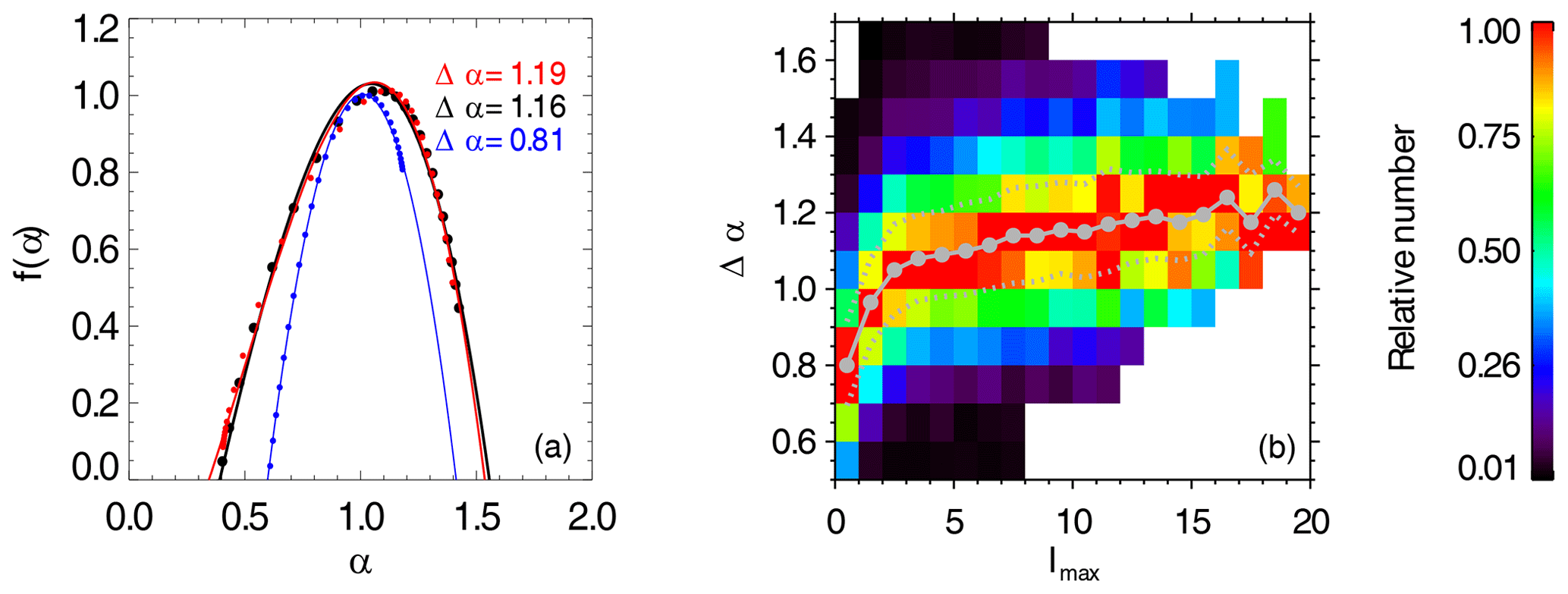
Figure 10 (a) Multifractal singularity spectra f(α) versus α observed in the slow wind (points), where red represents the intermittent interval shown in Fig. 4 (I_max=13.09), black represents the intermittent interval shown in Fig. 2 (I_max=4.10), and blue represents the quiet interval shown in Fig. 5 (I_max=1.44). The solid lines denote the cubic polynomial fit to the observations. The width of each singularity spectrum $\mathrm{\Delta }\mathit{\alpha }={\mathit{\alpha }}_{\max }-{\mathit{\alpha }}_{\min }$ is marked in the panel. (b) Joint distribution of I_max and Δα for the 33 261 intervals with ${\mathit{\lambda }}_{\mathrm{1}}/{\mathit{\lambda }}_{\mathrm{2}}>\mathrm{3}$. For a given pixel, the color denotes the relative number, which is the number of cases normalized by the maximum number in the corresponding I_max bin. The pixels containing no more than 10 cases are ignored. The solid gray circles represent average Δα in each I_max bin. The dotted gray lines represent the upper/lower quartiles.

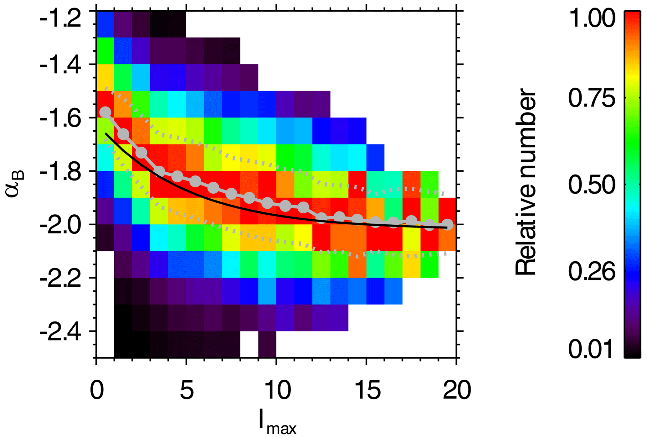
Figure 11 Joint distribution of the intermittency level I_max and magnetic spectral index α_B obtained using the “linear detrending preparation” method, plotted in the same format as Fig. 6b. The black curve is the exponential function ${\mathit{\alpha }}_B=\mathrm{0.4}\exp (-I_{\max }/\mathrm{5})-\mathrm{2.02}$ adopted from Fig. 6.

4.4 Linearly detrending data prior to FFT

When performing the FFT on the components of magnetic field data, we use a simple rectangular window (hereinafter referred to as the “no data preprocessing” method). This method could introduce extra discontinuity in the data that will add Fourier power to the magnetic PSD, as mentioned by Borovsky (2012) and Borovsky and Burkholder (2020). Following Borovsky (2012), we try linearly detrending each data interval prior to Fourier transformation (hereinafter referred to as the “linear detrending preparation” method), and we compare the result with that in Fig. 6 obtained using the no data preprocessing method.

Figure 11 presents (plotted in the same format as Fig. 6b) the joint distribution of the intermittency level I_max and magnetic spectral index α_B obtained using the linear detrending preparation method. The analytical relationship ${\mathit{\alpha }}_B=\mathrm{0.4}\exp (-I_{\max }/\mathrm{5})-\mathrm{2.02}$, adopted from Fig. 6, is superposed on the figure as a black curve for easier comparison. It is clear that, when I_max>12, the black curve coincides with the averaged magnetic spectral indices α_B (gray dots) well. However, when I_max<12, the averaged magnetic spectral indices α_B (gray dots) obtained from the linear detrending preparation method appear to be larger than those obtained from the no data preprocessing method (denoted by the black curve). The differences between them are about 0.01–0.06. This is consistent with Borovsky (2012), who mentioned that the no data preprocessing method leads to slightly steeper spectral indices. When looking at the upper/lower quartiles, we notice that the distribution of α_B in an I_max bin obtained using the linear detrending preparation method (e.g., ${\mathit{\alpha }}_B=-{\mathrm{1.90}}_{-\mathrm{0.14}}^{+\mathrm{0.15}}$ at I_max=8.5) is slightly wider than that obtained using the no data preprocessing method (e.g., ${\mathit{\alpha }}_B=-{\mathrm{1.93}}_{-\mathrm{0.12}}^{+\mathrm{0.13}}$ at I_max=8.5). The wider distribution for the linear detrending preparation method is also consistent with Borovsky (2012). Accordingly, we suggest that the magnetic spectral index changes slightly when using different data preprocessing methods, but our results with respect to the trend in the magnetic spectral index α_B versus the intermittency level I_max and the contribution of the intermittency to the magnetic spectra are robust.

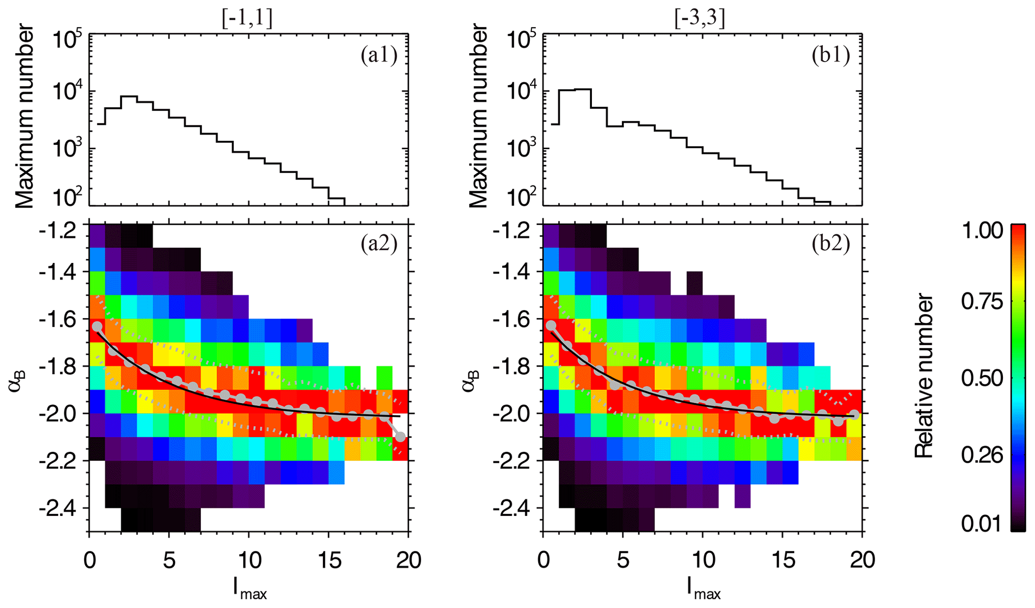
Figure 12 Panels (a1) and (a2) and panels (b1) and (b2) are plotted in the same format as Fig. 6 but for the respective PVI thresholds of $[-\mathrm{1},\mathrm{1}]$ and $[-\mathrm{3},\mathrm{3}]$ for identifying an intermittent interval. The black curves in panels (a2) and (b2) are both the exponential function ${\mathit{\alpha }}_B=\mathrm{0.4}\exp (-I_{\max }/\mathrm{5})-\mathrm{2.02}$, which is adopted from Fig. 6.

5 Conclusions

In this paper, we present, for the first time, the analytical relation between the magnetic spectral index α_B in the inertial range and the level of intermittency I_max at the timescale of τ=24 s in the slow solar wind. Data from Wind spacecraft observations between 2005 and 2013 are used for analysis. We preliminarily examine 56 398 intermittent structures using the criterion $\left|{\mathrm{PVI}}_i\right|>\mathrm{2}$ ($i=x,y,$ or z), with t_B and t_E being the beginning and ending instants of a structure, respectively. However, for more than half of the structures, the maximum I (I_max) during [t_B,t_E] (as marked by the two vertical dotted lines in Fig. 2) is not the maximum I during the corresponding plotted interval [t_B−150 s, t_E+150 s] (the whole plotted interval in Fig. 2). This means that, outside of [t_B,t_E], some other structures exist with an even higher level of intermittency during the interval [t_B−150 s, t_E+150 s]. We eliminate these kinds of intervals, during which the energy of the fluctuations is not dominated by the intermittent structure embedded in the center of it. In this way, we avoid the duplicate selection of the cases and also guarantee that both the intermittency level I_max and the magnetic spectral index α_B are closely related to the intermittent structure embedded in the middle of each interval. We then obtain 25 912 intermittent intervals. Subsequently, the cases with a higher fitting error of the magnetic power spectra (${\mathrm{\Delta }}_{{\mathit{\alpha }}_B}/{\mathit{\alpha }}_B>\mathrm{5}\mathit{\%}$) are eliminated, and 24 886 intermittent intervals are reserved for the statistical analysis.

Finally, we select 24 886 intermittent intervals and 17 386 quiet intervals from 46 slow-wind streams. Each intermittent interval lasts about 5–6 min with a dominant intermittent structure embedded in the center of it. The maximum I (I_max) of an intermittent structure is recorded as the intermittency level of the corresponding interval. The magnetic trace power spectrum of each interval is obtained by performing FFT on the high-resolution magnetic field data with $\mathrm{\Delta }{t}_{\mathrm{H}}=\mathrm{1}/\mathrm{11}$ s, and it is then linearly interpolated onto a uniformly spaced grid in the log–log space. The magnetic spectral index α_B is obtained by performing a least-squares fit on the interpolated spectrum between 0.01 and 0.3 Hz in the inertial range. The selected intervals all have relatively low fitting errors (${\mathrm{\Delta }}_{{\mathit{\alpha }}_B}/{\mathit{\alpha }}_B\le \mathrm{5}\mathit{\%}$), indicating that their magnetic power spectra have a good power-law shape.

The observed variation in the averaged spectral index α_B as a function of the intermittency level I_max is presented in Fig. 6b as solid gray circles. When I_max increases from 0.5 to 15.5, the magnetic power spectrum gets steeper and the averaged magnetic spectral index α_B decreases from $-{\mathrm{1.63}}_{-\mathrm{0.12}}^{+\mathrm{0.09}}$ to $-{\mathrm{1.99}}_{-\mathrm{0.11}}^{+\mathrm{0.09}}$. We also find that the averaged magnetic spectral index α_B changes more quickly at I_max≤3.5 than at $\mathrm{3.5}<I_{\max }\le \mathrm{15.5}$. When I_max gets larger, the magnetic spectral index stops decreasing and remains almost constant at ${\mathit{\alpha }}_B\approx -\mathrm{2}$. However, the dependence of the magnetic spectral index on the magnetic compressibility seems not to be significant, as shown in Figs. 7 and 8.

According to the observational result, an empirical relation is built up between the magnetic spectral index α_B and the intermittency level I_max as ${\mathit{\alpha }}_B=\mathrm{0.4}\exp (-I_{\max }/\mathrm{5})-\mathrm{2.02}$. The empirical relation is illustrated using the black curve in Fig. 6b. It gives the continuous variation in the magnetic spectral index α_B as a function of the intermittency level I_max. This relation will help people to easily estimate the contribution of the intermittency level to the magnetic spectral index, which implies the nature of the cascading process happening in the turbulence. It also supplies an observational constraint for numerical studies related to intermittency and spectral analysis of the solar wind turbulence. Moreover, from the aspect of theoretical study, the relation will help improve turbulence theories that contains intermittent structures.

We also check the sensitivity of the results based on the choice of the threshold for identifying an intermittent interval. The threshold is changed from the original PVI range of $[-\mathrm{2},\mathrm{2}]$ into two new respective ranges of $[-\mathrm{1},\mathrm{1}]$ and $[-\mathrm{3},\mathrm{3}]$. The results are shown in Fig. 12. Figure 12a1 and a2 correspond to the threshold of $[-\mathrm{1},\mathrm{1}]$ for identifying an intermittent interval, whereas Fig. 12b1 and b2 correspond to the threshold of $[-\mathrm{3},\mathrm{3}]$. Figure 12 is plotted in the same format as Fig. 6. The black curves in Fig. 12a2 and b2 are both the exponential function ${\mathit{\alpha }}_B=\mathrm{0.4}\exp (-I_{\max }/\mathrm{5})-\mathrm{2.02}$, which is adopted from Fig. 6. It is found that the black curve obtained from the original threshold of $[-\mathrm{2},\mathrm{2}]$ can still match the new results well. Therefore, our result shown in Fig. 6 is robust and is not sensitive to the choice of the threshold for identifying intermittent intervals.

Moreover, Sari and Ness (1969) mentioned that “The only change in the spectra for intervals containing a different number of discontinuities, or of discontinuities of differing magnitude, should be in the power levels, and not in the general spectral shape”. Based on the high-resolution data and sufficient samples observed by the Wind spacecraft, our results here provide observational evidence that the magnetic spectral shape (i.e., the spectral index in the inertial range) actually changes when the intermittency level of interval is different. Therefore, when researchers try to study the cascading process and evolution of the solar wind turbulence, it is very necessary to consider the effect of the intermittency level. In the future, we will also investigate the influence of the number of intermittent structures on the magnetic spectral shape. Additionally, it would also be interesting to establish the physical nature of the intermittent structures found in the slow-wind streams and to compare the result with those in the fast-wind streams (Wang et al., 2013).