the Creative Commons Attribution 4.0 License.
the Creative Commons Attribution 4.0 License.
 | 23 Sep 2021
Polar tongue of ionisation during geomagnetic superstorm
Dimitry Pokhotelov
Isabel Fernandez-Gomez
Claudia Borries
During the main phase of geomagnetic storms, large positive ionospheric plasma density anomalies arise at middle and polar latitudes. A prominent example is the tongue of ionisation (TOI), which extends poleward from the dayside storm-enhanced density (SED) anomaly, often crossing the polar cap and streaming with the plasma convection flow into the nightside ionosphere. A fragmentation of the TOI anomaly contributes to the formation of polar plasma patches partially responsible for the scintillations of satellite positioning signals at high latitudes. To investigate this intense plasma anomaly, numerical simulations of plasma and neutral dynamics during the geomagnetic superstorm of 20 November 2003 are performed using the Thermosphere Ionosphere Electrodynamics Global Circulation Model (TIE-GCM) coupled with the statistical parameterisation of high-latitude plasma convection. The simulation results reproduce the TOI features consistently with observations of total electron content and with the results of ionospheric tomography, published previously by the authors. It is demonstrated that the fast plasma uplift, due to the electric plasma convection expanded to subauroral mid-latitudes, serves as a primary feeding mechanism for the TOI anomaly, while a complex interplay between electrodynamic and neutral wind transports is shown to contribute to the formation of a mid-latitude SED anomaly. This contrasts with published simulations of relatively smaller geomagnetic storms, where the impact of neutral dynamics on the TOI formation appears more pronounced. It is suggested that better representation of the high-latitude plasma convection during superstorms is needed. The results are discussed in the context of space weather modelling.
- Article
(10624 KB) - Full-text XML
-
Supplement
(15930 KB) - BibTeX
- EndNote


In the course of a geomagnetic storm, large amounts of solar wind energy and momentum are deposited into the high-latitude ionosphere through the Joule dissipation of magnetosphere/ionosphere currents and auroral particle precipitation (Rodger et al., 2001). During the storm main phase a large positive dayside ionospheric plasma anomaly, known as the storm-enhanced density (SED), arises at sub-auroral mid-latitudes (Mendillo et al., 1972; Buonsanto, 1999; Immel and Mannucci, 2013). The morphologies of dayside SEDs have strong seasonal, local time, longitudinal, and other dependencies (Borries et al., 2015). A formation of the SED anomaly is largely (though not exclusively) attributed to the storm-time changes in plasma transport (Prölss, 1995, 2008; Immel and Mannucci, 2013), especially to the uplift of plasma to higher altitudes with longer recombination times. Storm-time changes in plasma/neutral composition and chemistry play greater roles in the formation of negative plasma anomalies, which are more common during the storm recovery phase (Rishbeth et al., 1987; Prölss and Werner, 2002).
The key physical mechanisms contributing to the storm-time plasma uplifts include (a) equatorward thermospheric neutral winds driven by the storm-time Joule dissipation (Anderson, 1976; Rishbeth, 1998) and (b) a vertical component of the electric E×B plasma convection expanded equatorward to mid-latitudes (Deng and Ridley, 2006; Heelis et al., 2009). Also, a horizontal plasma transport due to the poleward expansion of the equatorial plasma anomaly (Tsurutani et al., 2004) or due to the westward plasma drift caused by subauroral polarisation streams (Foster et al., 2007) has been invoked to explain the SED anomaly. However, the importance of the last two mechanisms, which involve substantial horizontal plasma transport over mid-latitudes, has been downplayed by Rishbeth et al. (2010) and Fuller-Rowell (2011), respectively, based on considerations of plasma transport times and global plasma density distributions. In this study the vertical uplifts due to (a) neutral winds and (b) expanded E×B convection are considered to be the key competing mechanisms for the generation of SED anomalies. We also note that this study does not aim to explain the formation of an SED anomaly.
The focal point of this study is the tongue of ionisation (TOI), which is a storm-time plasma density anomaly originating at the poleward edge of the SED anomaly, spreading anti-sunward across the polar cap and reaching the nightside auroral zone (Knudsen, 1974; Foster et al., 2005). The TOI anomaly has been observed during large geomagnetic storms using multiple radar systems (Foster et al., 2005) emphasising the role of cross-polar plasma transport by the enhanced E×B plasma convection flow. Using tomographic inversions of total electron content (TEC) observations, the 3D structure of the TOI anomaly has been revealed (Mitchell et al., 2008) and the role of dayside plasma uplift has been demonstrated (Yin et al., 2006). In situ satellite observations using ion drift instruments during the 20 November 2003 storm (Pokhotelov et al., 2008) suggested that the uplift can be attributed to the equatorward expansion of E×B convection flow. Storm-time observations of cross-polar plasma convection and plasma density using polar cap digital ionosondes (Pokhotelov et al., 2009) and SuperDARN radars (Thomas et al., 2013) demonstrated that sudden changes in the convection regime (e.g. due to rapid changes in the interplanetary magnetic field) can effectively disrupt the formation of a TOI anomaly. The fragmentation of a TOI anomaly is considered to be one of the mechanisms producing polar patches responsible for radio scintillations (e.g. Moen et al., 2013).
Earlier numerical simulations of the SED anomaly demonstrated competing roles of the plasma uplift mechanisms due to neutral winds and electric fields (e.g. Lin et al., 2005; Crowley et al., 2006; Swisdak et al., 2006). Since the mid-latitude SED anomaly provides a source of the uplifted dense plasma for the TOI anomaly, it is reasonable to assume that the same two mechanisms may control the formation of a TOI anomaly. However, the SED anomaly covers the entire local day–evening sector and often persists throughout the storm main phase and through an early part of the recovery phase, while the TOI anomaly is relatively narrow in longitude and persists for shorter times during the main phase. With recent developments of higher-resolution ionospheric circulation models (e.g. Maute, 2017), it became possible to simulate the dynamics of the TOI across the polar cap. Recently Liu et al. (2016) modelled the development of TOI anomalies during two comparable geomagnetic storms of March 2013 and March 2015 using the new release of the Thermosphere-Ionosphere Electrodynamics General Circulation Model (TIE-GCM) with 2.5∘ horizontal resolution. Based on the simulations, they concluded that the uplift and horizontal transport due to the E×B drifts generally dominate over other possible drivers, such as neutral winds and compositional/chemical changes. Klimenko et al. (2019) modelled the TOI dynamics during the March 2015 geomagnetic storm, concluding that neutral dynamics and compositional changes may contribute to the suppression of a TOI anomaly beyond the geomagnetic North Pole. Using an ultra-high-resolution (0.6∘) version of the TIE-GCM model, Dang et al. (2019) modelled the separation of the TOI anomaly into “double tongues” associated with morning and evening convection cells during the March 2013 storm event. However, these recent modelling studies simulated relatively moderate geomagnetic storms. The storm of March 2015, the largest in solar cycle 24, has a disturbance storm time (Dst) index minimum of −226 nT. Such storms are not in the category of “great storms”, commonly defined as having a Dst below nT (Kamide et al., 1997). The current study is an attempt to model the TOI formation with a physics-based ionospheric model during a great storm (superstorm) event. The magnetosphere–ionosphere interactions in general (Kamide et al., 1997) and the formation of SED/TOI anomalies in particular (Pokhotelov et al., 2008) can both be quantitatively and qualitatively different during great storms.
In this study we use an example of the 20 November 2003 geomagnetic superstorm to analyse key mechanisms responsible for the formation and evolution of the TOI anomaly. The 20 November 2003 storm provides an advantage of being an isolated event driven by a single coronal mass ejection (Zhang et al., 2007). It is among the largest geomagnetic storms observed by modern space/ground instrumentation, including Global Navigation Satellite Systems (GNSS). Early studies of this storm using radars (Foster et al., 2005) and GNSS tomography (Pokhotelov et al., 2008) revealed the dynamics and 3D morphology of the TOI anomaly. However, self-consistent numerical simulations of the TOI anomaly were not possible at that time due to resolution limits of the existing ionospheric models and other factors. In this study the high-resolution version of the TIE-GCM model is used to model the TOI anomaly, with the analysis focusing on possible roles of the E×B drifts and neutral winds. A comparison with earlier GNSS tomography reconstructions is presented as well as with TEC distributions using conventional geometric TEC mapping. Limitations of other ionospheric circulation models in reproducing the TOI anomaly are also discussed, including the models currently used by space weather services.
In terms of the equatorial ring current disturbance magnitude, the geomagnetic storm of 20 November 2003 was the largest storm of solar cycle 23 and one of the largest storms recorded by modern instruments, with the Dst index reaching a value of −422 nT (Zhang et al., 2007). The storm was an isolated event preceded by a ∼ 20 d period of relatively quiet geomagnetic activity. Following the interplanetary shock arrival at 08:35 UT on 20 November 2003, the main phase of the storm lasts until ∼ 19:00 UT. During the main phase, the north–south IMF component (Bz) turns strongly negative, reaching to below −50 nT, while the dawn–dusk IMF component (By) increases to +50 nT in the beginning of the main phase and then goes down and turns negative after 18:00 UT (Fig. 1). With the solar wind speed (VSW) exceeding 700 km/s, this IMF configuration should lead to a very strong two-cell plasma convection pattern. The observed IMF By change from positive to negative is expected to alter the east–west orientation of the “throat” (the entry region) of the cross-polar convection channel throughout the main phase (e.g. Sojka et al., 1994). During the main phase, the two-cell convection pattern expands dramatically to lower latitudes (to magnetic latitude), as also confirmed by in situ plasma drift measurements using the Defence Meteorological Satellite Program (DMSP) spacecraft (Pokhotelov et al., 2008). This expanded convection is expected to cause an anomalous vertical plasma transport at subauroral latitudes due to the resulting vertical component of E×B drift.
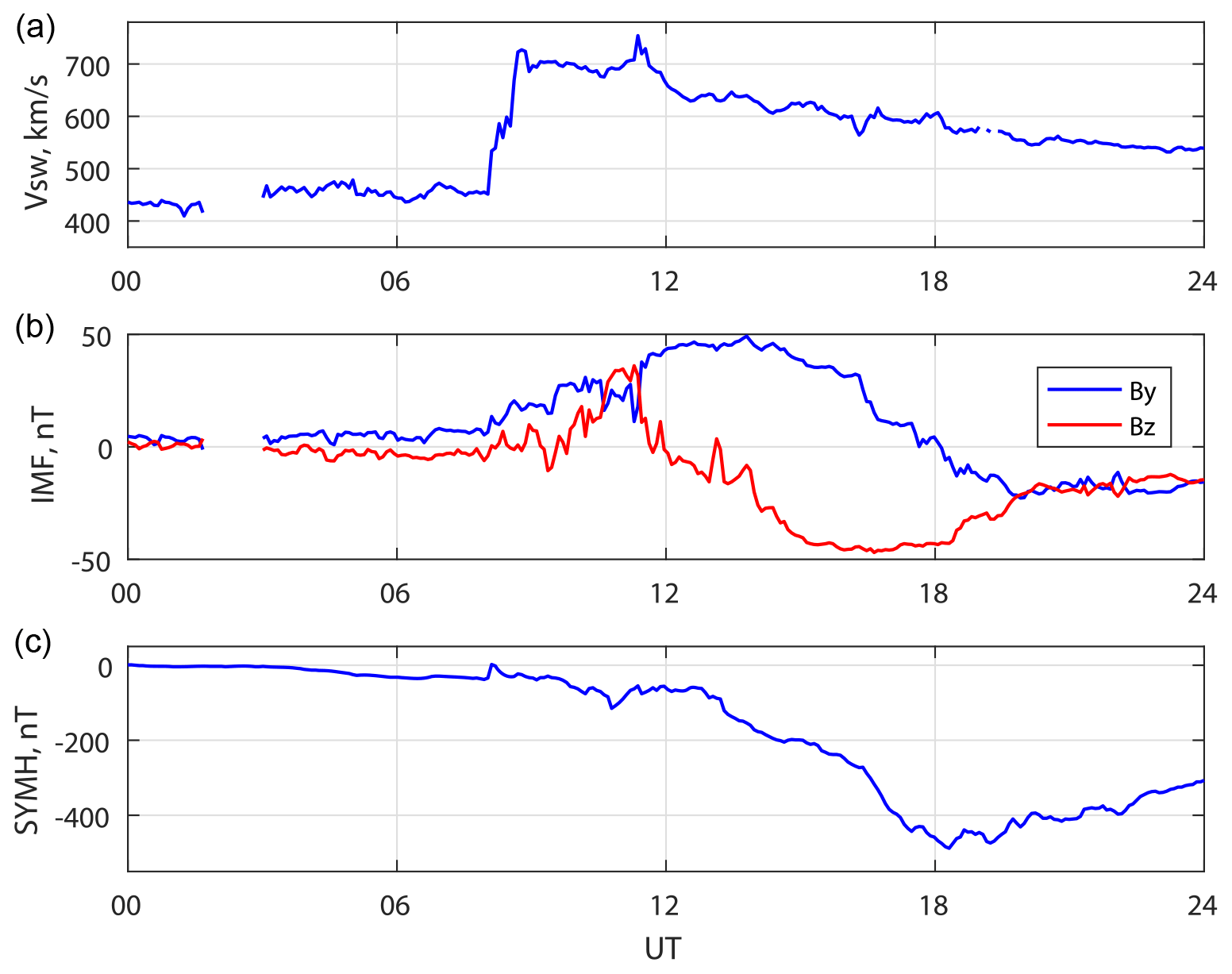
Figure 1Solar wind speed (a), interplanetary magnetic field components (b), and symmetric horizontal component disturbance index (c) during the 20 November 2003 storm.
To analyse the ionospheric dynamics during the 20 November 2003 storm, simulations have been performed using the TIE-GCM (Richmond et al., 1992; Qian et al., 2014). The TIE-GCM is a first-principle model simulating energy and momentum equations in the coupled thermosphere–ionosphere system. The current high-resolution version TIE-GCM v2.0 (Maute, 2017) uses the hydrostatic grid with 57 logarithmically spaced pressure levels ( scale height resolution), covering geopotential heights from ∼ 97 to ∼ 600 km, with uniform horizontal 2.5∘ grid resolution in longitude and latitude.
To facilitate the thermosphere/ionosphere forcing from above and below, the TIE-GCM should be coupled with external models. Mean horizontal neutral winds at the lower simulation boundary can be specified according to the Horizontal Wind Model (HWM07; Drob et al., 2008) and atmospheric tides are specified according to the Global Scale Wave Model (GSWM; Hagan and Forbes, 2002, 2003). Most relevant to the high-latitude storm dynamics, the plasma convection pattern is specified according to the statistical parameterisations of Heelis et al. (1982) or Weimer (2005). In this study, the Weimer parameterisation (Weimer, 2005) is used with the electrostatic potential expressed as a function of solar wind and IMF parameters measured upstream of the Earth's magnetosphere and time-shifted to the bow shock according to King and Papitashvili (2005).
The TIE-GCM simulation is performed throughout the 20 November 2003 storm after the 20 d initialisation run to reach the model equilibrium. Following the methodology of Liu et al. (2016), the simulated outputs of the 19 November 2003 quiet day are subtracted from the simulated 20 November 2003 storm day outputs. The resulting relative ΔTEC1 anomalies for the 20 November 2003 day are shown as a snapshot at 15:00 UT in Fig. 2 and as an animated sequence for the interval 10:00–23:00 UT in the Supplements (movie01.avi). For reference, absolute values of TEC are also shown in Fig. 2.
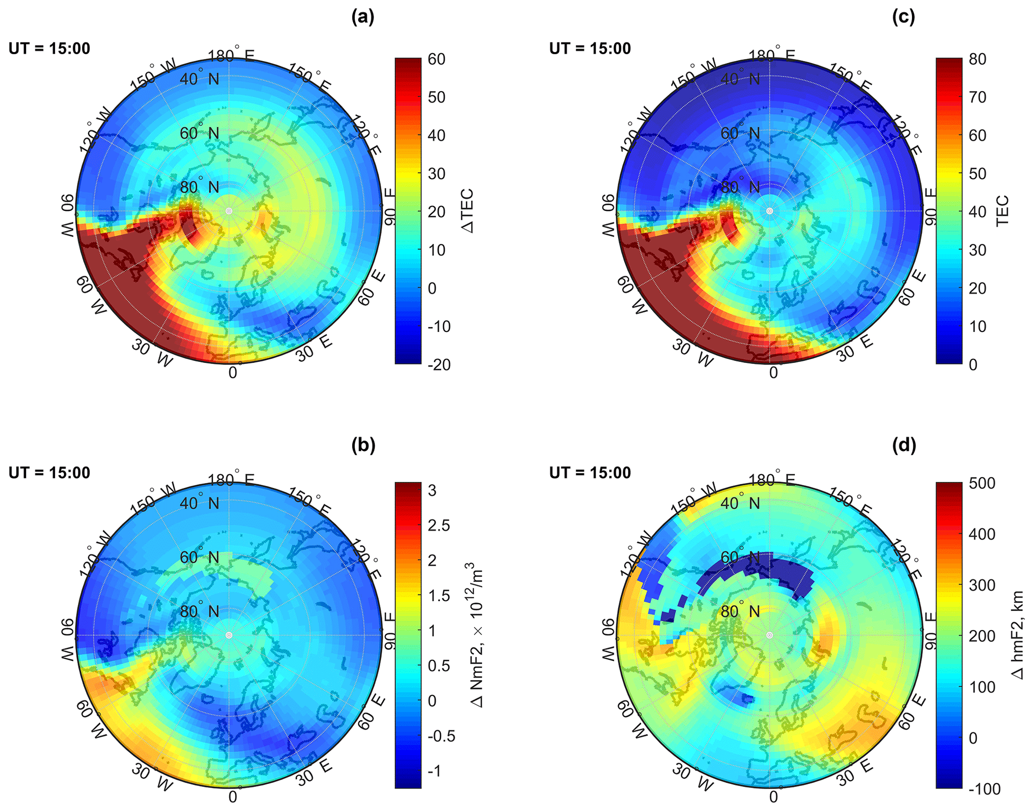
Figure 2Modelled TIE-GCM distributions of relative ΔTEC (a), plasma density at the F2 peak (b), absolute TEC (c) and the height of the F2 peak (d) at 15:00 UT 20 November 2003.
The following parameters relevant to storm-time plasma dynamics are also extracted from the TIE-GCM simulation. The height of the ionospheric F2 peak (hmF2) and plasma density at the F2 peak (NmF2) are shown in Fig. 2. Using the electrostatic potential (ϕ) given by the Weimer convection model, horizontal and vertical components of the plasma electric drift () are computed as vector products with the Earth's internal magnetic field (B). Expressed in geographic coordinates, northward meridional (VE×B) and vertical (WE×B) components of the electric drift are shown in Fig. 3 (a snapshot at 15:00 UT) and as an animated sequence for the interval 10:00–23:00 UT in the Supplements (movie02.avi). Meridional neutral winds (V) at pressure levels corresponding to ∼120 and ∼400 km geopotential heights and the Joule heating per unit mass (QJoule) are shown in Fig. 4 (a snapshot at 15:00 UT) and in the Supplements (movie03.avi).
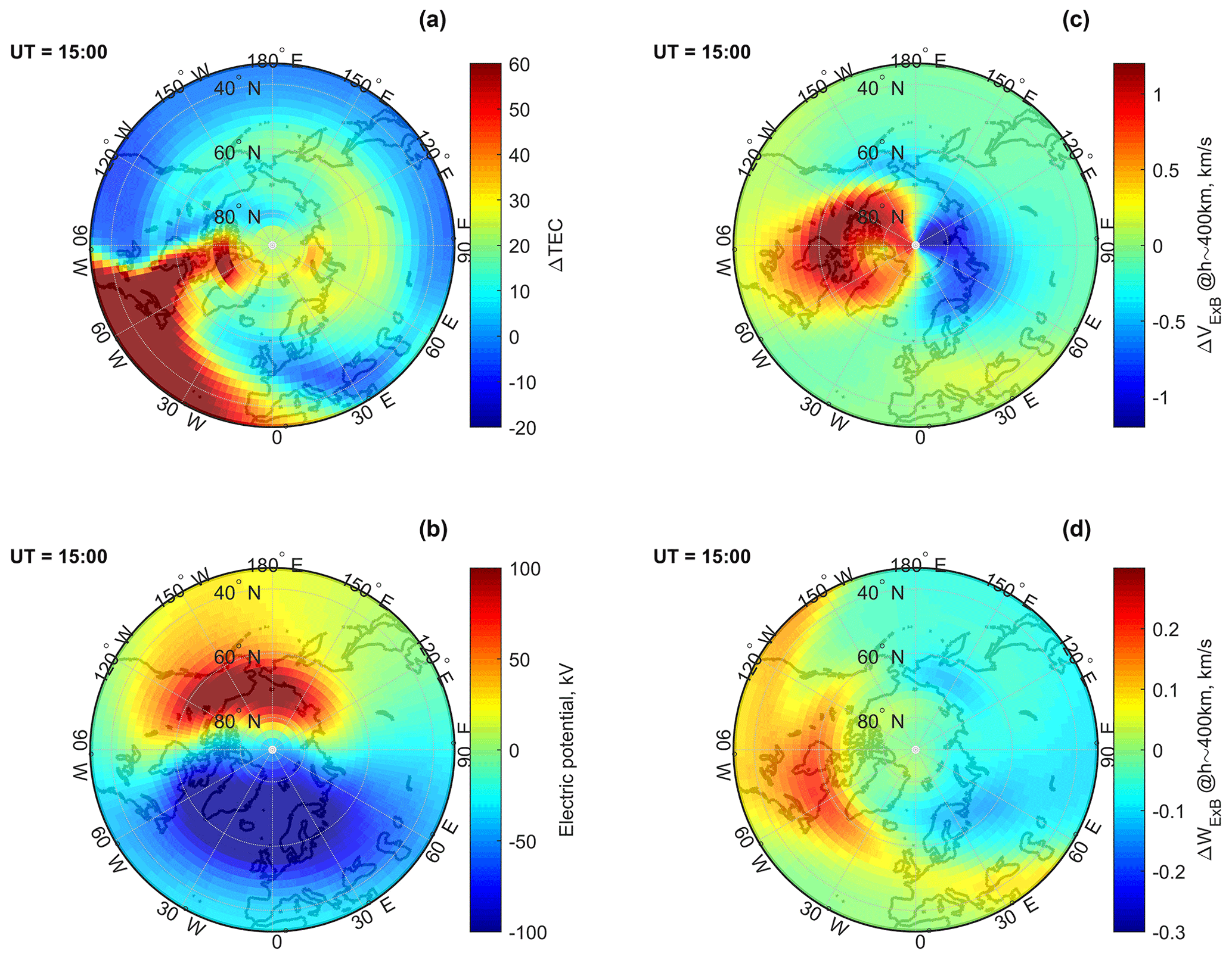
Figure 3Modelled TIE-GCM distributions of relative ΔTEC (a), electrostatic potential (b), and relative horizontal (c) and vertical (d) components of the E×B convection flow at 15:00 UT 20 November 2003.
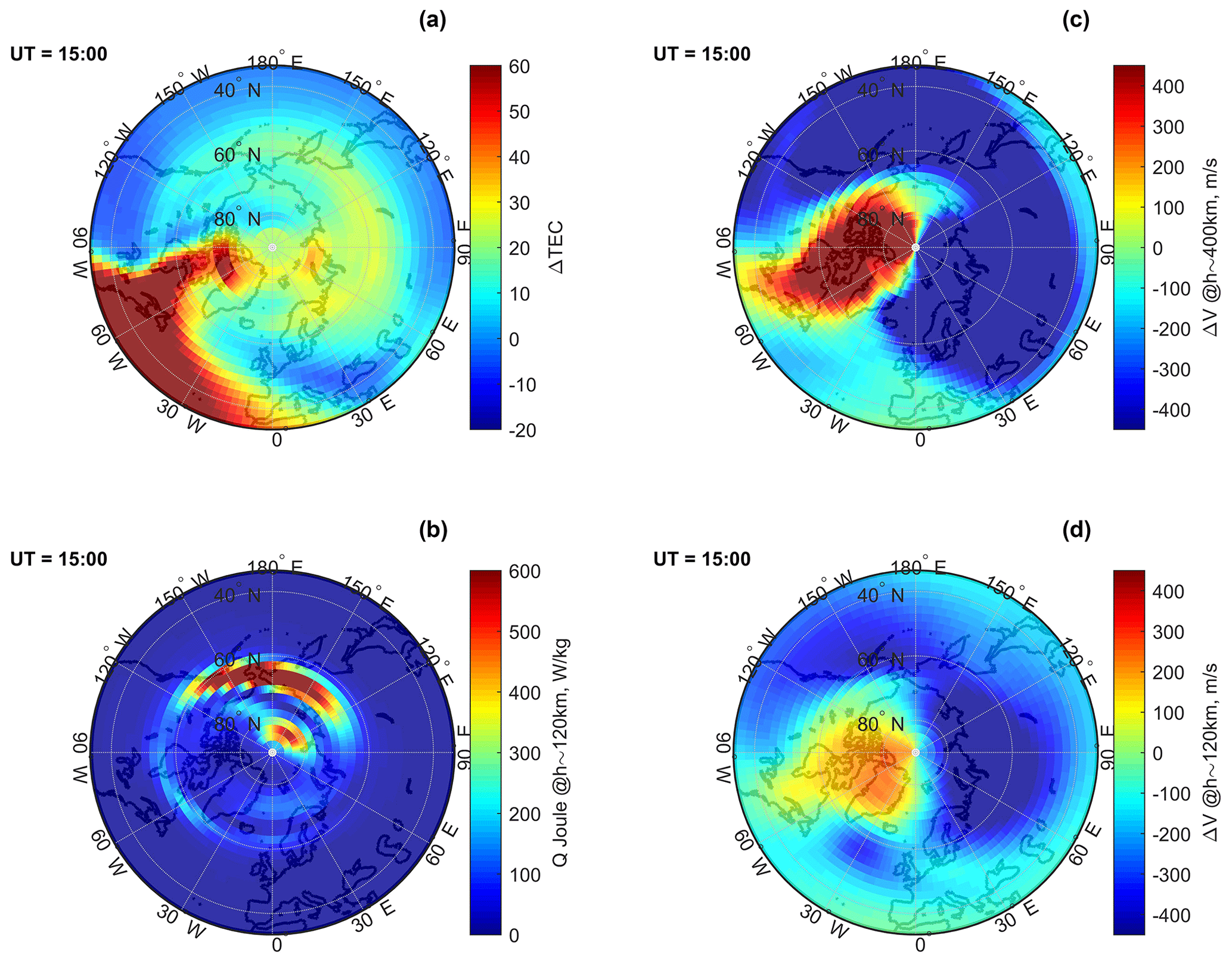
Figure 4Modelled TIE-GCM distributions of relative ΔTEC (b), Joule heating, and relative meridional neutral wind different levels (c)–(d) at 15:00 UT 20 November 2003.
Simulations of the 20 November 2003 storm with the Coupled Thermosphere Ionosphere Plasmasphere electrodynamics (CTIPe) model (Fuller-Rowell et al., 1996; Millward et al., 2001) have also been used in this study to compare to the TIE-GCM simulations described above. CTIPe is the first-principle model solving plasma and neutral dynamics on the hydrostatic grid with a resolution of in latitude and longitude, respectively, and 15 pressure levels in the vertical direction going from the lower boundary at ∼ 80 to ∼ 400 km in altitude. The atmospheric forcing is specified according to the Whole Atmosphere Model (WAM) (Akmaev et al., 2008). WAM fields (neutral temperature, zonal and meridional neutral winds) are averaged in every local hour sector of a given month and thus contain the monthly-averaged mean winds and tides. The high-latitude electrodynamic forcing is specified according to the statistical parameterisations of Weimer (2005). The capability of CTIPe to reproduce SED anomalies during the main phase of the 20 November 2003 superstorm has been demonstrated in Fernandez-Gomez et al. (2019) for the European sector. In this study, the extended CTIPe run has been used to analyse anomalies in the North American sector, with the results discussed in Sect. 5.4. The purpose is to see whether the operational CTIPe model reproduces similar features to the higher-resolution research model (TIE-GCM).
The radio signals transmitted by GNSS can be used to retrieve information about ionospheric plasma anomalies. Due to dispersive properties of the ionospheric plasma, GNSS signals carry information about the TEC along the signal trajectory. Using thin ionospheric shell approximation (e.g. Horvath and Crozier, 2007) and taking proper care of the receiver and transmitter biases, slant TEC observations by ground GNSS receivers can be converted into the 2D distributions of vertical TEC. GNSS-based maps of TEC, using the thin shell transformation, are available from the International GNSS Services (IGS) with typical grid resolutions of in latitude × longitude (Hernández-Pajares et al., 2009). IGS TEC maps can be directly compared to the results of numerical simulations, though one needs to be careful with artefacts caused by sparse/uneven distributions of ground GNSS receivers. Examples of IGS TEC maps during the 20 November 2003 storm are presented in Fig. 5, also showing a comparison with the distributions of absolute TEC simulated by the TIE-GCM. An animated sequence of absolute TEC maps from TIE-GCM simulations and from IGS services for the interval 11:00–23:00 UT 20 November 2003 is included in the Supplements (movie04.avi).
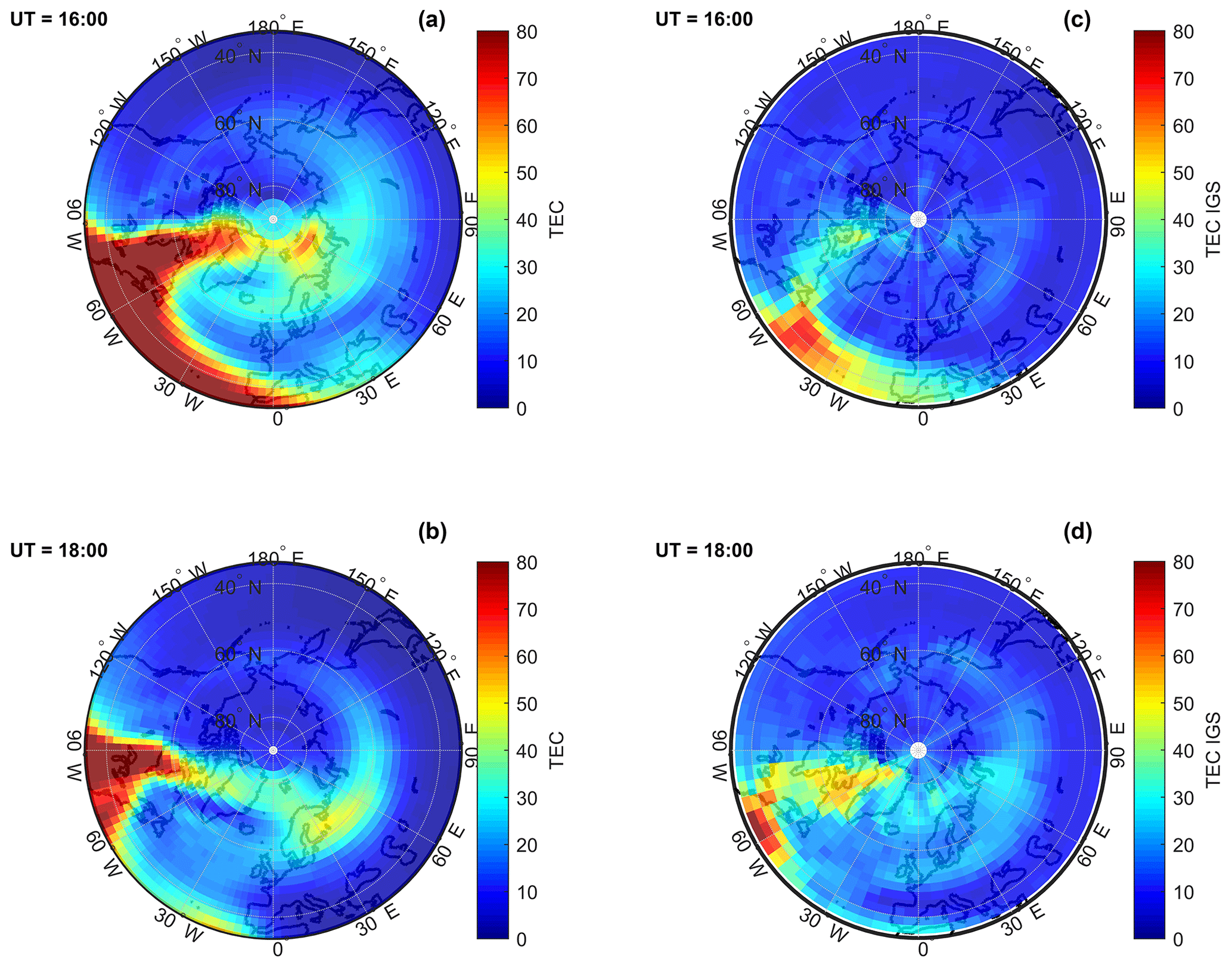
Figure 5TEC distributions obtained from TIE-GCM simulations (a, b) and from IGS services (c, d) at 16:00 UT (a, c) and 18:00 UT (b, d) during the 20 November 2003 storm.
A tomographic inversion of multiple slant TEC observations is also possible, yielding the 3D distribution of plasma density. The 3D time-dependent algorithm of ionospheric plasma tomography is described by Mitchell and Spencer (2003), and it has been previously applied to reconstruct the high-latitude plasma anomalies during the 20 November 2003 storm (Pokhotelov et al., 2008) using the network of 60 ground IGS receivers. Additional information about the E×B plasma drifts has been included in the tomographic algorithm using the Kalman filters with the Weimer convection model as a priori information (Spencer and Mitchell, 2007). The distributions of TEC obtained from the tomographic reconstructions were previously published and are presented in Fig. 6 of Pokhotelov et al. (2008) in the same format and at the same time moments (16:00 and 18:00 UT) as TEC distributions from TIE-GCM simulations and from IGS services shown here in Fig. 5.
5.1 Total electron content
Total electron content maps provide global coverage showing the morphology of plasma anomalies on ionospheric mesoscales comparable to the horizontal resolution of TIE-GCM simulations presented here (). However, the TEC mapping experiences potential problems at high latitudes due to (a) sparse/uneven distribution of ground GNSS receivers, (b) singularities of the latitude–longitude grid at the geographic poles, and (c) configuration of the GNSS satellite orbits. The network of ground IGS receiver stations available at polar latitudes during the 20 November 2003 storm is presented in Fig. 2 of Pokhotelov et al. (2008), showing separations between some of the polar cap receivers far greater than the desired horizontal resolutions. The inclination of GPS satellite orbits of (Samama, 2008) also contributes to the deficiencies of TEC reconstructions in the polar cap region. The tomographic reconstruction algorithm (Mitchell and Spencer, 2003; Spencer and Mitchell, 2007) partially mitigates these deficiencies by using rotated tomographic grids without the polar singularity and by including a priori information about plasma convection in the polar cap. Thus the tomographic reconstruction has advantages over the thin shell IGS TEC mapping, providing a more homogeneous solution across the polar cap region.
Taking into account the above limitations, we can compare the simulated TEC distributions with the results of TEC mapping and tomography. As shown in Fig. 5 and in the animation (movie04.avi), the TOI anomaly is visible in TEC maps (both from IGS and from the TIE-GCM model) starting from ∼ 12:00 UT, though the poleward extension of the SED anomaly appears at first some 20∘ further westward in the TIE-GCM simulations relative to the IGS TEC maps (southern tip of Greenland in the simulations vs. east of Iceland in IGS maps). The reasons for this mismatch in the local time/location of the TOI formation are not clear and will be discussed further in Sect. 5.4. One has to note that TEC reconstructions are not reliable over the Atlantic Ocean sector due to poor GNSS receiver coverage.
The main development of the TOI anomaly (from ∼ 13:00 to 18:00 UT) is seen over the eastern sector of the United States–Canada, spreading further anti-sunward over the geomagnetic North Pole and northern tip of Greenland. In simulations and in TEC observations, the TOI anomaly develops in the same longitudinal sector (60–90∘ W), though the simulated TOI appears narrower in longitude and more homogeneous in latitude. After 19:00 UT the TOI anomaly starts to disintegrate and disappear and the remains of the plasma are transported across the polar cap, merging into the nightside auroral TEC enhancement seen over the European sector. Overall, the location and general morphology of the simulated TOI anomaly is remarkably close to the IGS TEC observations and the tomography, except for the difference in the TOI onset time/location mentioned earlier. The amplitudes of modelled TEC anomalies (both SED and TOI) appear somewhat higher relative to the observations, confirming the assessment of Liu et al. (2016) that the TIE-GCM generally overestimates the magnitude of positive storm anomalies at high latitudes, though the specific reasons for this overestimation cannot be addressed here. The overestimation of TEC in TIE-GCM simulations, relative to IGS TEC maps, may reach up to 30–40 TEC units in the vicinity of the geomagnetic North Pole (Fig. 5). For the smaller geomagnetic storm of March 2015, TIE-GCM simulations overestimate the TOI anomaly by 10–15 TEC units relative to IGS TEC maps (see Fig. 4 in Liu et al., 2016, for comparison). IGS TEC maps are also expected to suffer from the lack of ground GNSS receivers in the Arctic Ocean sector. Thus, the comparison between the modelled TEC and the observed IGS TEC is questionable in the nightside region beyond the North Pole. The TIE-GCM grid singularity at the geographic North Pole may also lead to numerical problems in cross-polar plasma transport and continuity.
5.2 Plasma uplift dynamics
At first we analyse the dynamics of plasma uplift without looking into specific uplift mechanisms. As most of the ionospheric plasma is expected to be confined in the vicinity of the F2 peak, it is instructive to compare TEC distributions to the height and density of the F2 peak. The comparison (see Fig. 2 and the Supplements) confirms that the F2 peak plasma density (NmF2) largely mimics the behaviour of TEC. In contrast, the change in F2 peak height (ΔhmF2) shows a more complex behaviour. Substantial enhancements of hmF2 (up to 300 km) appear in the following longitude sectors (as referred to 15:00 UT 20 November 2003): (a) central part of the mainland USA west of 80∘ W, westward of the main SED anomaly; (b) eastern coast of Canada and towards the geomagnetic North Pole at 45–65∘ W, corresponding to the TOI location; and (c) eastern part of Europe and Central Asia east of 20∘ E, in the post-sunset sector. Out of these three major hmF2 enhancements, only the TOI-related enhancement (b) is accompanied by a clear increase in plasma density and TEC, while the other two enhancements are accompanied by negative density anomalies. The post-sunset enhancement in hmF2 (c) is considered to be related to a sudden significant increase in hmF2 reported in Borries et al. (2017), which is accompanied by an extreme increase in the equivalent slab thickness. The authors consider intensive plasma transport with strong vertical components at this period of time over the respective region. The most westward enhancement in hmF2 (a) is due to the early formation of an SED anomaly in that sector and does not have a clear connection to the TOI anomaly. Some secondary positive/negative anomalies in hmF2 are seen in conjunction/alignment with the auroral TEC anomalies and will not be discussed here. The main focus here is the clear enhancement of hmF2 coinciding with the positive anomaly in NmF2 and TEC at the poleward edge of the SED anomaly and the throat of the TOI anomaly, lasting from ∼ 14:00 to 19:00 UT.
5.3 Electrodynamic vs. neutral wind transport
We first focus on the comparison between the modelled relative TEC distributions and the electrodynamic transport parameters shown in Fig. 3 and in the Supplements. As indicated by the electric potential distributions, the high-latitude plasma convection pattern greatly expands equatorwards and develops the characteristic two-cell pattern following the southward IMF turn at 11:00–12:00 UT. The expanded two-cell convection pattern persists through the storm's main phase, reaching the maximum expansion at 17:00–18:00 UT around the minimum of the SYMH index. This is consistent with the DMSP satellite observations of E×B convection during this storm (see Figs. 5 and 6 in Pokhotelov et al., 2008). The comparison shows that the Weimer model used in TIE-GCM underestimates the degree of equatorward expansion. Due to IMF By being strongly positive in the early main phase (11:00–15:00 UT), the convection “throat” is initially oriented NW–SE, later changing its orientation to NE–SW, when the IMF By becomes negative around 18:00 UT. This change in orientation of the convective channel is clearly reflected in the shape of the TOI TEC anomaly. The influence of east–west convection asymmetry on the TOI anomaly due to the IMF By dynamics has been reported before (e.g. Sojka et al., 1994), and it requires further analysis, which is outside the scope of this study. The important feature of electrodynamic plasma transport is the enhancement in the vertical electric drift component (WE×B) seen at latitudes from 60∘ N down to 40–45∘ N, which accompanies the equatorward expansion of plasma convection. The vertical drift component arises from the E×B convection expanded to latitudes where dipolar magnetic field lines are far from vertical (e.g. Swisdak et al., 2006). The vertical electric drift maximises in the same longitudinal sector as the TOI anomaly. It maximises at the poleward edge of the SED anomaly and in the throat of the cross-polar convection channel (∼ 70∘ W, 50–60∘ N) but has a larger E–W extension (∼ 30–100∘ W) than the TOI anomaly itself. Additionally, enhanced vertical drifts are seen at ∼ 40 ∘ N in a broader range of longitudes extending into the central–western USA sector (west of 90∘ W). The amplitudes of vertical drifts of ∼ 200 m/s appear to be very large, but they are generally consistent with occasional storm-time measurements of large vertical plasma drifts by the mid-latitude Millstone Hill incoherent scatter radar (Yeh and Foster, 1990; Erickson et al., 2010; Zhang et al., 2017) and the uplifts of the F2 peak by ∼ 400 km within 1 h estimated from tomographic reconstructions during the main phase of the 30 October 2003 superstorm (Yin et al., 2006).
During storms, Joule heating in the auroral region changes thermospheric winds and generates so-called storm wind cells (Volland, 1983). The model results show (Fig. 4) the enhanced Joule heating near the throat region at about 60∘ N, but the amplitude is small compared to the Joule heating in the nightside auroral region ( W E). The heating-induced equatorward neutral winds are expected to cause plasma uplift at subauroral latitudes, contributing to the formation of SED (Rishbeth, 1998; Swisdak et al., 2006) and possibly TOI anomalies. The modelled distributions of meridional neutral winds (see Fig. 4 and the Supplements) clearly show enhancements of winds (200–300 m/s at 120 km height and up to 500 m/s at 400 km height) in the longitudinal sector of the TOI anomaly blowing in the anti-sunward (cross-polar) direction, even partially equatorwards of the heating region (60–80∘ W). Enhanced equatorward neutral winds are primarily seen in the central–western USA sector (west of 90∘ W). We also notice that at the early stage of the TOI formation (∼ 13:00 UT) the meridional neutral winds are nearly zero at the poleward edge of SED and at the throat of the convective channel but become polewards later on and appear at higher latitudes. This is an indication that at the poleward edge of SED and in the throat region, forcing from the enhanced E×B convection flow is stronger than the forcing from heating-induced winds. The cross-polar neutral wind is mainly driven by the plasma convection, thus forming the polar cap neutral tongue anomaly (Burns et al., 2004).
5.4 Relations to other modelling efforts and space weather applications
After comparing the electrodynamics and neutral wind dynamics, we conclude that the uplift due to the vertical component of enhanced E×B convection is the dominant mechanism forming the TOI anomaly. This is generally consistent with the conclusions of Liu et al. (2016), based on TIE-GCM modelling of two relatively smaller storms (with Dst minima of −132 and −226 nT) driven with the Weimer convection model. Liu et al. (2016) concluded that around the F2 region peak and above, the electric field transport is the dominant driver of positive SED/TOI anomalies, while at lower altitudes (∼ 280 km) neutral winds could play a major role in producing the positive anomalies. The dominant role of electrodynamic uplift/transport is also confirmed by Huba et al. (2017), who used the SAMI3 model driven with the Rice Convection Model (RCM), showing that the realistic TOI anomaly can be reproduced even without including the neutral wind dynamo. The dominant role of electrodynamic plasma uplift in the formation of the TOI anomaly does not rule out a complex interplay between electric convection, neutral winds, and other possible mechanisms responsible for the formation of a mid-latitude SED anomaly (e.g. Swisdak et al., 2006; Crowley et al., 2006), which is outside the scope of this study. It is also possible that during relatively smaller geomagnetic events, such as the March 2013 and March 2015 storms (Liu et al., 2016; Klimenko et al., 2019), the effects of neutral winds and compositional changes are more pronounced compared to the superstorm case presented here. For instance, we do not observe such clear suppression of the TOI anomaly beyond the geomagnetic North Pole, as noticed by Klimenko et al. (2019) during the March 2015 storm. In contrast to Liu et al. (2016), showing that at lower altitudes (∼ 280 km) the neutral wind effects may cause the enhancement of TOI density (see Fig. 7 in Liu et al., 2016), we obtain strongly poleward neutral winds at all altitudes down to ∼ 120 km (see Fig. 4), implying negative or no contribution of the neutral wind effects to the TOI formation.
The conclusions above are subject to the right choice of high-latitude E×B plasma convection model. The Weimer parameterisation (Weimer, 2005) used here to drive the TIE-GCM simulations and also for the earlier tomographic reconstructions (Spencer and Mitchell, 2007; Pokhotelov et al., 2008) should provide a realistic response to the rapid changes in solar wind/IMF conditions, which could be missing in the case of Heelis parameterisation (Heelis et al., 1982) based on the 3 h resolution planetary index (Kp). Our TIE-GCM simulations repeated for the 20 November 2003 storm using the Heelis convection parameterisation (not shown here but available on request) demonstrated relatively poor agreement with IGS TEC maps and tomography. Pokhotelov et al. (2008) demonstrated that the statistical Weimer parameterisation may not be able to capture the true extent of equatorward expansion of the E×B convection pattern during the superstorm. The mismatch between the times/longitudes of the early TOI formation (the TOI anomaly appears earlier in time and more eastward in IGS TEC maps relative to the TIE-GCM simulations, as noted in Sect. 5.1) is likely due to this underestimation of the E×B expansion. Simulations driven with more realistic convection patterns obtained from e.g. radar network observations during a specific storm (Wu et al., 2015) or from assimilative models (Lu et al., 2016) may be needed to overcome these deficiencies.
While it is clear that the numerical setup of the CTIPe model (namely, the coarse resolution of 18∘ in longitude) is not ideal for analysing the TOI anomaly, it is beneficial to discuss the results of this model in the context of space weather applications as the CTIPe is currently used for operational analysis and forecast by the US National Oceanic and Atmospheric Administration Space Weather Prediction Center – https://www.swpc.noaa.gov/models (last access: 21 September 2021) (Codrescu et al., 2012). The CTIPe simulation of the 20 November 2003 storm by Fernandez-Gomez et al. (2019) extended to the North American sector does not show clear TOI developments, though the CTIPe reproduces enhanced neutral wind patterns in the polar cap (Fig. A1) similar to those modelled by the TIE-GCM. On the other hand, Pryse et al. (2009) demonstrated that the CTIP model (Millward et al., 1996) was able to reproduce some features of the TOI anomaly consistent with ionospheric tomography when the simulation was driven by the SuperDARN radar observations of plasma convection. The use of SuperDARN data for driving the simulations was not addressed here but should be exploited in the future.
A fragmentation of the TOI anomaly due to IMF dynamics and other mechanisms has long been attributed to the formation of polar cap plasma patches (Sojka et al., 1994; Carlson et al., 2004). Climatological studies of ionospheric GNSS scintillations at high latitudes (e.g. Prikryl et al., 2015) demonstrate strong correlations with the plasma patches, especially near noon in the cusp region and near midnight, i.e. near the exit from a cross-polar convection channel2. One has to note that polar patches are formally defined as drifting F-region plasma irregularities with horizontal scales ∼ 100 km and densities 2–10 times above the background and could also be formed during geomagnetically quiet times (Moen et al., 2013). Nevertheless, the TOI anomaly is expected to be a dominant source of the high-latitude GNSS disruptions during geomagnetic storms, and it needs to be addressed in space weather applications.
The feeding mechanisms of the TOI anomaly have been analysed using the simulations of the geomagnetic superstorm of 20 November 2003, which have been conducted using the high-resolution version of the TIE-GCM ionospheric circulation model with the Weimer parameterisation of high-latitude E×B plasma convection. The simulation results are compared to the IGS TEC maps and to the results of ionospheric GNSS tomography for this storm event, published earlier by the authors (Pokhotelov et al., 2008). The main conclusions are summarised as the following.
- a.
The TIE-GCM simulations reproduce the development of the polar TOI anomaly consistently with the IGS TEC maps and the tomographic TEC reconstructions. Differences between the model and observations are seen in the early formation of the TOI anomaly and in the magnitude/longitudinal extent of the TEC anomaly across the polar cap. The results of TIE-GCM simulations are qualitatively consistent with earlier modelling of less severe geomagnetic storms with the TIE-GCM and other ionospheric models (Liu et al., 2016; Huba et al., 2017). The TIE-GCM substantially overestimates the amplitude of the TOI anomaly in the polar cap (up to 40 %–50 % overestimation in TEC units) relative to IGS TEC maps, which is generally consistent with the TIE-GCM simulations of smaller storms (Liu et al., 2016). The large uplift velocities shown by the TIE-GCM near the poleward edge of the SED anomaly and in the convection throat agree with earlier ionospheric tomography results and with radar observations of vertical drifts during large storms. The noted differences between the modelled TEC and IGS TEC maps can be attributed to the model deficiencies (especially the E×B convection parameterisations during storms) and to poor GNSS data coverage in the polar cap. More rigorous data–model comparisons using more recent storms with better GNSS coverage are needed.
- b.
Simulated distributions of the plasma and neutral dynamics demonstrate that the plasma uplifts of ∼ 200 m/s due to the high-latitude E×B plasma convection expanded to mid-latitudes appear to be the dominant mechanism responsible for the formation of the TOI anomaly. The neutral winds, enhanced during the storm, show the pattern which is not able to actively contribute to the TOI formation. This contrasts with the published simulations of relatively smaller geomagnetic storms (Liu et al., 2016; Klimenko et al., 2019), when neutral winds play a substantial role in forming and/or suppressing the TOI anomaly, especially at lower altitudes (Liu et al., 2016). We also show that the SED anomaly at mid-latitudes is likely to be influenced by both neutral wind and electrodynamic transport mechanisms, which is consistent with earlier simulations.
- c.
Comparisons between the TIE-GCM and CTIPe model show that the lower-resolution CTIPe model, currently used for space weather operations, is not able to reproduce the TOI anomaly correctly. On the other hand, TIE-GCM simulation of the TOI anomaly also has clear deficiencies. Better model representation of the E×B plasma convection during extreme geomagnetic storms is needed.
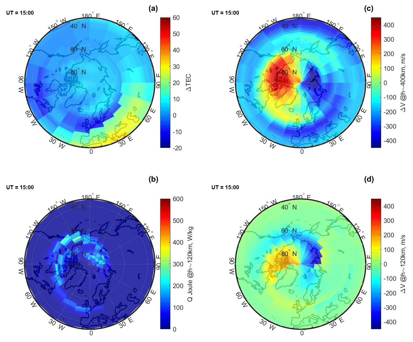
Figure A1Modelled distributions of relative ΔTEC (a), Joule heating (b), and relative meridional neutral winds at different levels (c)–(d) at 15:00 UT 20 November 2003 obtained from the CTIPe simulations.
Solar wind data and geomagnetic indices are available from the NASA OMNIWeb portal http://omniweb.gsfc.nasa.gov (last access: 21 September 2021) (NASA, 2021a). IGS total electron content data are available from the NASA CDAWeb portal https://cdaweb.gsfc.nasa.gov/pub/data/gps (last access: 21 September 2021) (NASA, 2021b). TIE-GCM is an open-source model available from the NCAR High Altitude Observatory https://www.hao.ucar.edu/modeling/tgcm (last access: 21 September 2021) (National Center for Atmospheric Research, 2021). The complete outputs of TIE-GCM simulations for the 20 November 2003 storm performed at the German Aerospace Center (DLR) are available upon request to the corresponding author.
The supplement related to this article is available online at: https://doi.org/10.5194/angeo-39-833-2021-supplement.
DP performed TIE-GCM simulations and compiled the manuscript. IFG performed CTIPe simulations and analysed IGS TEC data. CB provided expertise on mid-latitude ionospheric storm response and directed the study.
The authors declare that they have no conflict of interest.
Publisher's note: Copernicus Publications remains neutral with regard to jurisdictional claims in published maps and institutional affiliations.
The authors are grateful to Philip Erickson from MIT Haystack Observatory for providing insights into storm-time observations of vertical plasma drifts by the Millstone Hill incoherent scatter radar. The authors would like to thank Mariangel Fedrizzi and Mihail Codrescu from the NOAA Space Weather Prediction Center for providing details of the atmospheric forcing in CTIPe simulations.
The article processing charges for this open-access publication were covered by the German Aerospace Center (DLR).
This paper was edited by Dalia Buresova and reviewed by two anonymous referees.
Akmaev, R. A., Fuller-Rowell, T. J., Wu, F., Forbes, J. M., Zhang, X., Anghel, A. F., Iredell, M. D., Moorthi, S., and Juang, H.-M.: Tidal variability in the lower thermosphere: Comparison of Whole Atmosphere Model (WAM) simulations with observations from TIMED, Geophys. Res. Lett., 35, L03810, https://doi.org/10.1029/2007GL032584, 2008. a
Anderson, D.: Modeling the midlatitude F-region ionospheric storm using east-west drift and a meridional wind, Planet. Space Sci., 24, 69–77, https://doi.org/10.1016/0032-0633(76)90063-5, 1976. a
Borries, C., Berdermann, J., Jakowski, N., and Wilken, V.: Ionospheric storms – A challenge for empirical forecast of the total electron content, J. Geophys. Res.-Space, 120, 3175–3186, https://doi.org/10.1002/2015JA020988, 2015. a
Borries, C., Jakowski, N., Kauristie, K., Amm, O., Mielich, J., and Kouba, D.: On the dynamics of large-scale traveling ionospheric disturbances over Europe on 20 November 2003, J. Geophys. Res.-Space, 122, 1199–1211, https://doi.org/10.1002/2016JA023050, 2017. a
Buonsanto, M. J.: Ionospheric Storms – A Review, Space Sci. Rev., 88, 563–601, https://doi.org/10.1023/A:1005107532631, 1999. a
Burns, A., Wang, W., Killeen, T., and Solomon, S.: A “tongue” of neutral composition, J. Atmos. Sol.-Terr. Phys., 66, 1457–1468, https://doi.org/10.1016/j.jastp.2004.04.009, 2004. a
Carlson Jr., H. C., Oksavik, K., Moen, J., and Pedersen, T.: Ionospheric patch formation: Direct measurements of the origin of a polar cap patch, Geophys. Res. Lett., 31, L08806, https://doi.org/10.1029/2003GL018166, 2004. a
Codrescu, M. V., Negrea, C., Fedrizzi, M., Fuller-Rowell, T. J., Dobin, A., Jakowsky, N., Khalsa, H., Matsuo, T., and Maruyama, N.: A real-time run of the Coupled Thermosphere Ionosphere Plasmasphere Electrodynamics (CTIPe) model, Space Weather, 10, 02001, https://doi.org/10.1029/2011SW000736, 2012. a
Crowley, G., Hackert, C. L., Meier, R. R., Strickland, D. J., Paxton, L. J., Pi, X., Mannucci, A., Christensen, A. B., Morrison, D., Bust, G. S., Roble, R. G., Curtis, N., and Wene, G.: Global thermosphere-ionosphere response to onset of 20 November 2003 magnetic storm, J. Geophys. Res.-Space, 111, A10S18, https://doi.org/10.1029/2005JA011518, 2006. a, b
Dang, T., Lei, J., Wang, W., Wang, B., Zhang, B., Liu, J., Burns, A., and Nishimura, Y.: Formation of Double Tongues of Ionization During the 17 March 2013 Geomagnetic Storm, J. Geophys. Res.-Space, 124, 10619–10630, https://doi.org/10.1029/2019JA027268, 2019. a
Deng, Y. and Ridley, A. J.: Role of vertical ion convection in the high-latitude ionospheric plasma distribution, J. Geophys. Res.-Space, 111, A09314, https://doi.org/10.1029/2006JA011637, 2006. a
Drob, D. P., Emmert, J. T., Crowley, G., Picone, J. M., Shepherd, G. G., Skinner, W., Hays, P., Niciejewski, R. J., Larsen, M., She, C. Y., Meriwether, J. W., Hernandez, G., Jarvis, M. J., Sipler, D. P., Tepley, C. A., O'Brien, M. S., Bowman, J. R., Wu, Q., Murayama, Y., Kawamura, S., Reid, I. M., and Vincent, R. A.: An empirical model of the Earth's horizontal wind fields: HWM07, J. Geophys. Res.-Space, 113, A12304, https://doi.org/10.1029/2008JA013668, 2008. a
Erickson, P., Goncharenko, L., Nicolls, M., Ruohoniemi, M., and Kelley, M.: Dynamics of North American sector ionospheric and thermospheric response during the November 2004 superstorm, J. Atmos. Sol.-Terr. Phys., 72, 292–301, https://doi.org/10.1016/j.jastp.2009.04.001, 2010. a
Fernandez-Gomez, I., Fedrizzi, M., Codrescu, M. V., Borries, C., Fillion, M., and Fuller-Rowell, T. J.: On the difference between real-time and research simulations with CTIPe, Adv. Space Res., 64, 2077–2087, https://doi.org/10.1016/j.asr.2019.02.028, 2019. a, b
Foster, J., Rideout, W., Sandel, B., Forrester, W., and Rich, F.: On the relationship of SAPS to storm-enhanced density, J. Atmos. Sol.-Terr.l Phys., 69, 303–313, https://doi.org/10.1016/j.jastp.2006.07.021, 2007. a
Foster, J. C., Coster, A. J., Erickson, P. J., Holt, J. M., Lind, F. D., Rideout, W., McCready, M., van Eyken, A., Barnes, R. J., Greenwald, R. A., and Rich, F. J.: Multiradar observations of the polar tongue of ionization, J. Geophys. Res.-Space, 110, A09S31, https://doi.org/10.1029/2004JA010928, 2005. a, b, c
Fuller-Rowell, T. J.: Storm-time response of the thermosphere-ionosphere system, in: Aeronomy of the Earth's Atmosphere and Ionosphere, IAGA Spec. Sopron Book Ser., Vol. 2, edited by: Abdu, M. A. and Pancheva, D., Springer, Dordrecht, 419–434, https://doi.org/10.1007/978-94-007-0326-1_32, 2011. a
Fuller-Rowell, T. J., Rees, D., Quegan, S., Moffett, R. J., Codrescu, M. V., and Millward, G. H.: A coupled thermosphere‐ionosphere model (CTIM), in: STEP Handbook of Ionospheric Models, edited by: Schunk, R. W., Utah State University, Logan, 217–238, 1996. a
Hagan, M. E. and Forbes, J. M.: Migrating and nonmigrating diurnal tides in the middle and upper atmosphere excited by tropospheric latent heat release, J. Geophys. Res.-Atmos., 107, 4754, https://doi.org/10.1029/2001JD001236, 2002. a
Hagan, M. E. and Forbes, J. M.: Migrating and nonmigrating semidiurnal tides in the upper atmosphere excited by tropospheric latent heat release, J. Geophys. Res.-Space, 108, 1062, https://doi.org/10.1029/2002JA009466, 2003. a
Heelis, R. A., Lowell, J. K., and Spiro, R. W.: A model of the high-latitude ionospheric convection pattern, J. Geophys. Res.-Space Phys., 87, 6339–6345, https://doi.org/10.1029/JA087iA08p06339, 1982. a, b
Heelis, R. A., Sojka, J. J., David, M., and Schunk, R. W.: Storm time density enhancements in the middle-latitude dayside ionosphere, J. Geophys. Res.-Space, 114, A03315, https://doi.org/10.1029/2008JA013690, 2009. a
Hernández-Pajares, M., Juan, J. M., Sanz, J., Orus, R., Garcia-Rigo, A., Feltens, J., Komjathy, A., Schaer, S. C., and Krankowski, A.: The IGS VTEC maps: a reliable source of ionospheric information since 1998, J. Geodesy, 83, 263–275, https://doi.org/10.1007/s00190-008-0266-1, 2009. a
Horvath, I. and Crozier, S.: Software developed for obtaining GPS-derived total electron content values, Radio Sci., 42, RS2002, https://doi.org/10.1029/2006RS003452, 2007. a
Huba, J. D., Sazykin, S., and Coster, A.: SAMI3-RCM simulation of the 17 March 2015 geomagnetic storm, J. Geophys. Res.-Space, 122, 1246–1257, https://doi.org/10.1002/2016JA023341, 2017. a, b
Immel, T. J. and Mannucci, A. J.: Ionospheric redistribution during geomagnetic storms, J. Geophys. Res.-Space, 118, 7928–7939, https://doi.org/10.1002/2013JA018919, 2013. a, b
Kamide, Y., McPherron, R. L., Gonzalez, W. D., Hamilton, D. C., Hudson, H. S., Joselyn, J. A., Kahler, S. W., Lyons, L. R., Lundstedt, H., and Szuszczewicz, E.: Magnetic Storms: Current Understanding and Outstanding Questions, American Geophysical Union (AGU), 28, 1–20, https://doi.org/10.1029/GM098p0001, 1997. a, b
King, J. H. and Papitashvili, N. E.: Solar wind spatial scales in and comparisons of hourly Wind and ACE plasma and magnetic field data, J. Geophys. Res.-Space, 110, A02104, https://doi.org/10.1029/2004JA010649, 2005. a
Klimenko, M. V., Zakharenkova, I. E., Klimenko, V. V., Lukianova, R. Y., and Cherniak, I. V.: Simulation and Observations of the Polar Tongue of Ionization at Different Heights During the 2015 St. Patrick's Day Storms, Space Weather, 17, 1073–1089, https://doi.org/10.1029/2018SW002143, 2019. a, b, c, d
Knudsen, W. C.: Magnetospheric convection and the high-latitude F2 ionosphere, J. Geophys. Res., 79, 1046–1055, https://doi.org/10.1029/JA079i007p01046, 1974. a
Lin, C. H., Richmond, A. D., Heelis, R. A., Bailey, G. J., Lu, G., Liu, J. Y., Yeh, H. C., and Su, S.-Y.: Theoretical study of the low- and midlatitude ionospheric electron density enhancement during the October 2003 superstorm: Relative importance of the neutral wind and the electric field, J. Geophys. Res.-Space, 110, A12312, https://doi.org/10.1029/2005JA011304, 2005. a
Liu, J., Wang, W., Burns, A., Solomon, S. C., Zhang, S., Zhang, Y., and Huang, C.: Relative importance of horizontal and vertical transports to the formation of ionospheric storm-enhanced density and polar tongue of ionization, J. Geophys. Res.-Space, 121, 8121–8133, https://doi.org/10.1002/2016JA022882, 2016. a, b, c, d, e, f, g, h, i, j, k, l, m
Lu, G., Richmond, A. D., Lühr, H., and Paxton, L.: High-latitude energy input and its impact on the thermosphere, J. Geophys. Res.-Space, 121, 7108–7124, https://doi.org/10.1002/2015JA022294, 2016. a
Maute, A.: Thermosphere-Ionosphere-Electrodynamics General Circulation Model for the Ionospheric Connection Explorer: TIEGCM-ICON, Space Sci. Rev., 212, 523–551, https://doi.org/10.1007/s11214-017-0330-3, 2017. a, b
Mendillo, M., Papagiannis, M. D., and Klobuchar, J. A.: Average behavior of the midlatitude F-region parameters NT, Nmax, and τ during geomagnetic storms, J. Geophys. Res., 77, 4891–4895, https://doi.org/10.1029/JA077i025p04891, 1972. a
Millward, G., Müller-Wodarg, I., Aylward, A., Fuller-Rowell, T., Richmond, A., and Moffett, R.: An investigation into the influence of tidal forcing on F region equatorial vertical ion drift using a global ionosphere-thermosphere model with coupled electrodynamics, J. Geophys. Res.-Space, 106, 24733–24744, https://doi.org/10.1029/2000ja000342, 2001. a
Millward, G. H., Moffett, R. J., Quegan, S., and Fuller-Rowell, T. J.: A coupled thermosphere-ionosphere-plasmasphere model (CTIP), in: STEP Handbook of Ionospheric Models, edited by: Schunk, R. W., Utah State University, Logan, 239–279, 1996. a
Mitchell, C. N. and Spencer, P. S. J.: A three-dimensional time-dependent algorithm for ionospheric imaging using GPS, Ann. Geophys., 46, 687–696, https://doi.org/10.4401/ag-4373, 2003. a, b
Mitchell, C. N., Yin, P., Spencer, P. S. J., and Pokhotelov, D.: Ionization Dynamics During Storms of the Recent Solar Maximum in Midlatitude Ionospheric Dynamics and Disturbances, American Geophysical Union (AGU), Geophys. Monogr. Ser., 181, 83–90, https://doi.org/10.1029/181GM09, 2008. a
Moen, J., Oksavik, K., Alfonsi, L., Daabakk, Y., Romano, V., and Spogli, L.: Space weather challenges of the polar cap ionosphere, J. Space Weather Space Clim., 3, A02, https://doi.org/10.1051/swsc/2013025, 2013. a, b
NASA: OMNIWeb Data Service [data set], available at: http://omniweb.gsfc.nasa.gov (last access: 21 September 2021), 2021a. a
NASA: CDAWeb Data Service [data set], available at: https://cdaweb.gsfc.nasa.gov/pub/data/gps, (last access: 21 September 2021), 2021b. a
National Center for Atmospheric Research: High Altitude Observatory [code], available at: https://www.hao.ucar.edu/modeling/tgcm, last access: 21 September 2021. a
Pokhotelov, D., Mitchell, C. N., Spencer, P. S. J., Hairston, M. R., and Heelis, R. A.: Ionospheric storm time dynamics as seen by GPS tomography and in situ spacecraft observations, J. Geophys. Res.-Space, 113, A00A16, https://doi.org/10.1029/2008JA013109, 2008. a, b, c, d, e, f, g, h, i, j, k
Pokhotelov, D., Mitchell, C. N., Jayachandran, P. T., MacDougall, J. W., and Denton, M. H.: Ionospheric response to the corotating interaction region-driven geomagnetic storm of October 2002, J. Geophys. Res.-Space, 114, A12311, https://doi.org/10.1029/2009JA014216, 2009. a
Prikryl, P., Jayachandran, P. T., Chadwick, R., and Kelly, T. D.: Climatology of GPS phase scintillation at northern high latitudes for the period from 2008 to 2013, Ann. Geophys., 33, 531–545, https://doi.org/10.5194/angeo-33-531-2015, 2015. a
Prölss, G. W.: Ionospheric F-region storms, in: Handbook of Atmospheric Electrodynamics II, edited by: Volland, H., CRC Press, Boca Raton, https://doi.org/10.1201/9780203713297, 195–248, 1995. a
Prölss, G. W.: Ionospheric Storms at Mid-Latitude: A Short Review, in: Midlatitude Ionospheric Dynamics and Disturbances, American Geophysical Union (AGU), Geophys. Monogr. Ser., 181, 9–24, https://doi.org/10.1029/181GM03, 2008. a
Prölss, G. W. and Werner, S.: Vibrationally excited nitrogen and oxygen and the origin of negative ionospheric storms, J. Geophys. Res.-Space, 107, 1016, https://doi.org/10.1029/2001JA900126, 2002. a
Pryse, S. E., Whittick, E. L., Aylward, A. D., Middleton, H. R., Brown, D. S., Lester, M., and Secan, J. A.: Modelling the tongue-of-ionisation using CTIP with SuperDARN electric potential input: verification by radiotomography, Ann. Geophys., 27, 1139–1152, https://doi.org/10.5194/angeo-27-1139-2009, 2009. a
Qian, L., Burns, A. G., Emery, B. A., Foster, B., Lu, G., Maute, A., Richmond, A. D., Roble, R. G., Solomon, S. C., and Wang, W.: The NCAR TIE-GCM: A Community Model of the Coupled Thermosphere/Ionosphere System, in: Modeling the Ionosphere-Thermosphere System, American Geophysical Union, Geophys. Monogr. Ser., 201, 73–83, https://doi.org/10.1002/9781118704417.ch7, 2014. a
Richmond, A. D., Ridley, E. C., and Roble, R. G.: A thermosphere/ionosphere general circulation model with coupled electrodynamics, Geophys. Res. Lett., 19, 601–604, https://doi.org/10.1029/92GL00401, 1992. a
Rishbeth, H.: How the thermospheric circulation affects the ionospheric F2-layer, J. Atmos. Sol.-Terr. Phys., 60, 1385–1402, https://doi.org/10.1016/S1364-6826(98)00062-5, 1998. a, b
Rishbeth, H., Fuller-Rowell, T. J., and Rodger, A. S.: F-layer storms and thermospheric composition, Phys. Scripta, 36, 327–336, https://doi.org/10.1088/0031-8949/36/2/024, 1987. a
Rishbeth, H., Heelis, R. A., Makela, J. J., and Basu, S.: Storming the Bastille: the effect of electric fields on the ionospheric F-layer, Ann. Geophys., 28, 977–981, https://doi.org/10.5194/angeo-28-977-2010, 2010. a
Rodger, A. S., Wells, G. D., Moffett, R. J., and Bailey, G. J.: The variability of Joule heating, and its effects on the ionosphere and thermosphere, Ann. Geophys., 19, 773–781, https://doi.org/10.5194/angeo-19-773-2001, 2001. a
Samama, N.: Global Positioning: Technologies and Performance, Wiley, Hoboken, 2008. a
Sojka, J. J., Bowline, M. D., and Schunk, R. W.: Patches in the polar ionosphere: UT and seasonal dependence, J. Geophys. Res.-Space, 99, 14959–14970, https://doi.org/10.1029/93JA03327, 1994. a, b, c
Spencer, P. S. J. and Mitchell, C. N.: Imaging of fast moving electron density structures in the polar cap, Ann. Geophys., 50, 427–434, https://doi.org/10.4401/ag-3074, 2007. a, b, c
Swisdak, M., Huba, J. D., Joyce, G., and Huang, C.-S.: Simulation study of a positive ionospheric storm phase observed at Millstone Hill, Geophys. Res. Lett., 33, L02104, https://doi.org/10.1029/2005GL024973, 2006. a, b, c, d
Thomas, E. G., Baker, J. B. H., Ruohoniemi, J. M., Clausen, L. B. N., Coster, A. J., Foster, J. C., and Erickson, P. J.: Direct observations of the role of convection electric field in the formation of a polar tongue of ionization from storm enhanced density, J. Geophys. Res.-Space, 118, 1180–1189, https://doi.org/10.1002/jgra.50116, 2013. a
Tsurutani, B., Mannucci, A., Iijima, B., Abdu, M. A., Sobral, J. H. A., Gonzalez, W., Guarnieri, F., Tsuda, T., Saito, A., Yumoto, K., Fejer, B., Fuller-Rowell, T. J., Kozyra, J., Foster, J. C., Coster, A., and Vasyliunas, V. M.: Global dayside ionospheric uplift and enhancement associated with interplanetary electric fields, J. Geophys. Res.-Space, 109, A08302, https://doi.org/10.1029/2003JA010342, 2004. a
Volland, H.: Dynamics of the disturbed ionosphere, Space Sci. Rev., 34, 327–335, https://doi.org/10.1007/BF00175287, 1983. a
Weimer, D. R.: Improved ionospheric electrodynamic models and application to calculating Joule heating rates, J. Geophys. Res.-Space, 110, A05306, https://doi.org/10.1029/2004JA010884, 2005. a, b, c, d
Wu, Q., Emery, B. A., Shepherd, S. G., Ruohoniemi, J. M., Frissell, N. A., and Semeter, J.: High-latitude thermospheric wind observations and simulations with SuperDARN data driven NCAR TIEGCM during the December 2006 magnetic storm, J. Geophys. Res.-Space, 120, 6021–6028, https://doi.org/10.1002/2015JA021026, 2015. a
Yeh, H.-C. and Foster, J. C.: Storm time heavy ion outflow at mid-latitude, J. Geophys. Res.-Space, 95, 7881–7891, https://doi.org/10.1029/JA095iA06p07881, 1990. a
Yin, P., Mitchell, C., and Bust, G.: Observations of the F region height redistribution in the storm-time ionosphere over Europe and the USA using GPS imaging, Geophys. Res. Lett., 33, L18803, https://doi.org/10.1029/2006GL027125, 2006. a, b
Zhang, J., Richardson, I. G., Webb, D. F., Gopalswamy, N., Huttunen, E., Kasper, J. C., Nitta, N. V., Poomvises, W., Thompson, B. J., Wu, C.-C., Yashiro, S., and Zhukov, A. N.: Solar and interplanetary sources of major geomagnetic storms (Dst ≤−100 nT) during 1996–2005, J. Geophys. Res.-Space, 112, 1314–1337, https://doi.org/10.1029/2007JA012321, 2007. a, b
Zhang, S.-R., Erickson, P. J., Zhang, Y., Wang, W., Huang, C., Coster, A. J., Holt, J. M., Foster, J. F., Sulzer, M., and Kerr, R.: Observations of ion-neutral coupling associated with strong electrodynamic disturbances during the 2015 St. Patrick's Day storm, J. Geophys. Res.-Space, 122, 1314–1337, https://doi.org/10.1002/2016JA023307, 2017. a
- Abstract
- Introduction
- Geomagnetic storm of 20 November 2003
- Simulations of the storm
- Total electron content from GNSS mapping and tomography
- Discussion
- Summary and conclusions
- Appendix A
- Data availability
- Author contributions
- Competing interests
- Disclaimer
- Acknowledgements
- Financial support
- Review statement
- References
- Supplement